A generalized output pruning algorithm for matrix-vector multiplication and its application to compute pruning discrete cosine transform

A Generalized Output Pruning Algorithm for Matrix-

Vector Multiplication and Its Application to Compute

Pruning Discrete Cosine Transform

Yuh-Ming Huang, Ja-Ling Wu, IEEE Senior Member, and Chi-Lun Chang Communications and Multimedia Laboratory

Dept. of Computer Science and Information Engineering National Taiwan University,Taipei, Taiwan

E-Mail: [email protected] or [email protected]

Abstract

-

In this paper, a generalized output pruning algorithm for matrix- vector multiplication is proposed first. Then the application of the proposed pruning algorithm to compute pruning Discrete Cosine Transform (DCT) is addressed. It is shown that, for a given decomposition of the matrix of the transform kernel and the pruning pattern, the unnecessary operations for computing an output pruning DCT can be eliminated thoroughly by using the proposed algorithm.

I. INTRODUCTION

Recently, a lot of one-dimensional (l-D) and two-dimensional (2-D) fast pruning DCT algorithms, for computing only the lower-frequency components, have been proposed in [1],[2],[3]. However, to the most of our knowledge, no known generalized pruning method can be directly applied to any orthogonal discrete transform, such as DCT, Discrete Fourier Transform (DFT), Discrete Hartley Transform (DHT),

. .

.,

etc. In this paper, a generalized output pruning algorithm for computing matrix-vector multiplication of any order is presented. It is shown that, for a given decomposition of the matrix, the unnecessary operations can be eliminated thoroughly. The efficient Pruning DCT algorithm can then be derived based on the prescribed pruning algorithm. Of course, the applicability of the proposed output p q i n g algorithm is not limited to DCT, actually, it can be applied to all well-known discrete orthogonal transforms, such as DFT, DHT, and Discrete Sine Transform (DST). However, in this write-up, pruning DCT algorithm is our only focus.

I1 A GENERALIZED OUTPUT PRUNING ALGORITHM

FOR MATRIX-VECTOR MULTIPLICATION

Consider the operation of a general matrix-vector multiplication of order N, say D,=A,,,xB N, and assume only partial multiplication outputs Dj (where

1

I

j I N ) are required. It follows that we can speed up the aforecited computation by pruning the unnecessary operations.

a product of a sequence of more-sparse matrices of the same order, that is, ANxN=

n

ckx

,

.

Then, the operation AN,Nx BN can be computed as

k-1

i = O

C:xN

xCLx,

X*..XC,~,

k-l

xB,,

where

CkxN

is more sparse than ANxN in general. By the associative property of matrix-vector multiplication, DN can be computed recursively as follows.

B i

=

B,

i

B,

=

Ck$

x

Bf;;',l<

i

5

k.

(1) k

D,

=

B,

. .

1

Since there are k stages of matrix-vector multiplication of order N in (l), no matter what kind of output pruning pattern is, kxN bits are required to record whether each

BF

has to be computed or not, where

Bf;'

is the inner-product of the j-th row vector of

C i i i

and the output vector

B:'

of the previous stage.

In this section, a more efficient algorithm for computing output-pruning matix-vector multiplication is presented. In this algorithm, only

rlog(k

+

1)1xN bits are required to record whether the partial results

BY

has to be computed or not. In other words, we need an array, say M of order N with each entry of

[lo&

+

1)1

bits in size, to record which operations are required or unnecessary.

If the computation of DN[i] is necessary, then initially let M[i]=O; otherwise let M[i]=255 or a large integer. The final value of each entry of M will evolve gradually through the computation of

cixN

to that of theci;, and will be pre-computed and stored with respect to the charactelistics of the concerned matrix

ckxN

, described as follows.

7 (A) Encoding Processes : \

Let T be a control or threshold parameter and its value is set to be zero, is a permutation matrix, that is for any vector V, of order N, the result of the matrix-vector multiplication

CkxN

XV, is just a position swapping of V,. In t h l s case, the entries of M are unchanged in

value but permuted according to the inverse permutation matrix (

CLxN

)-

',

and the value of T is unchanged, neither. initially.

<2> If

CLxN

is a diagonal matrix, that is, all the entries of

cLxN

are equal to zero except the diagonal components. In this case, the values of each entry of M and T will keep unchanged.

<3> If

chxN

is a general diagonal matrix, that is, all the diagonal components of it are not equal to zero and no constraint is set to the non- diagonal components. In this case, the value of T will be increased by one. The value of T (equal to TJ is used as a threshold for indicating the fact that: in the matrix-vector multiplication stage, say

CkxN

x

B;-’-’

=

B;-i

,

some output entry

Bi-i’s

is unnecessary (i.e. M[s] =

255), whereas the entry

Bi-i-”s

of the input vector

Bi-i-’

is required to compute some output entry

Bk-i’r.

That is, the s-th input entry

B;-i-”s

has to be computed correctly before dealing with the matrix- vector multiplication

ckxN

x

Bk-i-’,

but after then, the s-th output entry

Bf,-i’s

is no use for later stages. In other words, if M[r] < T,, and M[s] =

255, then we set M[s] = T,.

<4> If

ChxN

can be decomposed into a product of a general diagonal matrix and a permutation matrix, or vice versa. In this case, the array M will be processed by using the merged methodologies presented in <1> and <3>. <5> The other matrix forms which don’t belong to those of the above four

types are categorized as type <5>. Notice that those matrices discussed in

<1>, <2>, and <3> are special subsets of <4>. Hence, by definition, those matrices of type <5> can’t be decomposed into a product of a general diagonal matrix and a permutation matrix. Moreover, according to the following two corollaries, we will deduce that each matrix of type <5> is a linearly ’dependent matrix.

Corollary 1. If a matrix of size NxN cannot be decomposed into a product of a

general diagonal matrix and a permutation matrix of the same sue, then its determinant is equal to 0.

ProoJ We can prove this corollary by induction on N; however, we omit the

details due to page limit.

Corollary 2. If the determinant of a matrix H of size NxN is equal to 0, then H is a linearly dependent matrix.

Hence, the matrix discussed in <5> is linearly dependent. Since the determinant has the following property: If

Then

k-1

Therefore, by corollary 2 we know that ANxN is linearly dependent if

CkxN

is a linearly dependent matrix. Therefore, for any well-defined discrete transform matrix ANxN, which is linearly independent, it will never be categorized as a type

<5> matrix.

For the sake of convenience, those sets composed of the matrices discussed in <1>, <2>, <3>, and <4> are respectively denoted by P, D, GD, and PGD.

As we have obtained the final values for each entry of M through the computation of

cixN

to that of theck;, , then with the help of M, all the unnecessary operations for the computation of

C i x N

x

C;,,

x

-

x

C&!,

x

B,

can be eliminated thoroughly. The values of all the entries of M will keep unchanged during this process, but may just be permuted in certain occasions. Let the final accumulated value of T be denoted by Tp This means, among those matrices,

CkxN

OSiSk-1, there are T, matrices belong to GD or PGD. In other words, after the matrix decomposition. the value Tf is pre-computable.

Now, let us show how the unnecessary operations for the computation of

C i x N

x

ChXN

x . - - x

CNxN

x

B,

can be eliminated thoroughly with the aid of M and T.

k-1

(B)

Decoding Process :

First, let T = Tp The elimination processes for unnecessary operations are deduced gradually through the computation of

Ci:;

x

B ,

to that of the

C i x N

x

Bk-’.

<I> If

Cfv,,

E P (the permutation matrix set), then the entries of M will be swapped according to the permutation pattern defined by

ckxN

.

<2> If

C i x N

E D (the diagonal matrix set), then the j-th output

BL-i’’

needs to be computed only when M b ] I T, otherwise it can be left out for pruning the unnecessary operations.

<3> If

CkxN

E .GD (the general diagonal matrix set), then the j-th output

Bi-i’’

needs to be computed only when Mb]< T, otherwise it can be left out for pruning the unnecessary operations. Furthermore, the value of T will be decreased by one in this case.

set), it follows that

C i x N

can be decomposed into a product of a general diagonal matrix D, and a permutation matrix P, (or vice versa). Then, the entries of M will be permuted according to the P, first, and the j-th output

Bi-’”

has to be computed only when Mb]< T, otherwise it can be left out for pruning

.

Of course, the value of T will also be decreased by one in this case.

The above statements described the detailed procedures of the proposed pruning algorithm. Because the final value of T, i.e. T,, will not be greater thank, only

[log(k

+

1)l.N

bits are required to record the evolution process of M. The correctness of the proposed algorithm can be verified by corollary 3 and lemma 1.

Corollary 3. Let AN, (=

n

ckxN

) be a linearly independent matrix. From the proposedsalgorithm, it can be deduced that, in the computation of ANXNx BN , the j-th entry

%U]

of the input vector BN is necessary only when Mb] I

TI.

Proof: We can prove this corollary by induction on

k;

however, we omit the details due to page limit.

Lemma I . Let A N x N ( = n C ; I x N ) be a linearly independent matrix. Then all the unnecessary operations can be eliminated thoroughly by the above proposed pruning algorithm.

Proof We can prove this Lemma by induction on

k;

however, we omit the details due to page limit.

k-1

i=O

k-1

i=O

From Lemma 1, for a linearly independent matrix ANxN, we know that the unnecessary operations can be eliminated thoroughly when only the partial outputs of the matrix-vector multiplication AN,, xBN are required. But, for a special pruning pattern, does there exist another scheme which can be used to further reduce the number of required operations. In the next corollary, we show that the number of required operations cannot be reduced by just utilizing the permutation technique. Moreover, for

CNxN

E PGD, the gain of pruning will not be changed even if we apply a different decomposition to

cNxN

.

And this will be shown in Lemma 2.

Corollary 4. Let ANxN be a linearly independent matrix and

P,

be a permutation matrix. For any pruning pattern, on computing of the following expressions AN,NxBN

,

(ANxNPc)( P;’&), and P,( P;’ANxN)BN

,

the simplification gains

obtained from pruning the unnecessary operations will be the same.

pruning algorithm, the simplification gain will keep unchanged even though we apply a different decomposition to the matrix

CLxN

(E

PGD)

.

Proof: This lemma can be proved by examining all possible components of

CLxN

,

we omit the details also due to page limit.

- -

1 0 0 1 0 0 0 1 0 0 1 0 0 0 I X 0 1 0 1 0 1 0 1 0 0

_{- _}

Therefore, in the proposed algorithm, for a given decomposition of the matrix AN,, , the simplification gain is always the same even if we have applied some modifications to the decomposition of the matrix

cbxN.

On the other hand, more effective decomposition of the matrix ANxN is necessary if we want to obtain better simplification gain.

- 2 . 3 0 0 0 0 0 5.0 0 0 0 0 0 -0.4 0 0 0 0 0 4 . 7 0 0 0 0 0 3 . 2

111. A

Concrete Example

-

-

0 1 0 1 0 1 0 1 0 0 x 0 0 0 1 0 0 1 0 0 1 1 1 0 0 0

-

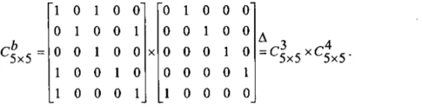
In general, the proposed general output pruning algorithm is suitable for the matrix-vector multiplication of any type: integer, real, or complex. Consider the matrix-vector multiplication of A sxsxB as an example, where

c t x 5 = 0

4

x

5

=

-

-

o o o l o r l o l o o

0 0 1 0 0 0 1 0 1 0 0 0 0 1 x 0 0 1 0 0 0 1 0 0 0 1 0 0 1 0

-

1 0 0 0 0 1 0 0 0 1

_{- -}

and B is an arbitary 5x 1 vector.

Let the above three decomposed matrices be denoted by

c&,

cix5

,

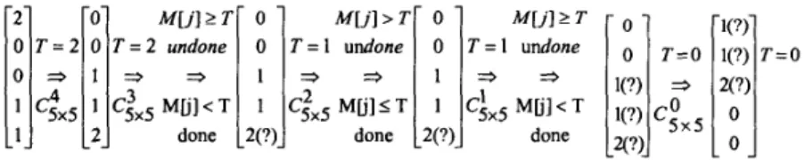
and respectively. Suppose only the last two entries of AsxSxB5 are required. According to the proposed approach, we set

M=

[255,255,255,0,0] and T=O,

initially. Because

Ctx5

and

csxs

b E PGD,

c:x,,

and

c.

can be respectively

A O 1

b CSx5 = X - 1 0 1 0 0 0 1 0 0 1 0 0 1 0 0 1 0 0 1 0 1 0 0 0 1 0 1 0 0 0 ' 0 0 1 0 0 0 0 0 1 0 0 0 0 0 1 1 0 0 0 0

-

-

- - - - - 255 0 0 0 255 T = O 0 T = O 0 T = l 0 0 Cgx5 255 CiX5 1 C52x5 1 0 255 255 255 2 5 5 3 2 5 5 = 1 3

-

-

-

-

-

-

-

-A 3 4 = c 5 x 5 x c 5 x 5 .

- -

- -

0 2 T = l 0 T = 2 OT=2=Tf 1 3 1 3 0 CZx5 1 Cs",5 1 2 1

- _

_ -

Through the computation of

C!x5

to that of

c;x5,

the values of each entry of the array M and threshold parameter T can be obtained gradually through the following five steps, as shown in Fig. 1.

Figure 1. The evolution of the array M and the threshold parameter T. Now, the array M and the threshold parameter T can be used to facilitate the output pruning computation of the matrix-vector multiplication A,,,xB, more efficiently. That is, the unnecessary operations can be eliminated thoroughly through the following five steps of the decoding process, as shown in Fig. 2. Step 1: Since

c;x5

E P, the value of T is kept unchanged (=2) and the entries of

pattern defined by the matrix

C:x5.

Step 2: Since

c:x5

E GD and M[4]22, the 4-th output (marked as ? in Fig. 2) will be left out for pruning and the other outputs are kept for later computation. Moreover, the value of T is decreased by 1 (=l).

Step 3: Since

c:x5

E D and M[j] I 1, 0 1 j 1 4 , the j-th outputs are necessary. The values of T and M are kept unchanged

Step 4: Since

cix5

E GD, M[2] 2 1 and M[3] 2 1, the 2nd and the 3rd outputs

(marked as ? in Fig. 2) will be left out for pruning and only the 0-th and the 1st outputs are kept for later computation. Moreover, the value of T is decreased by 1 (=O).

Step 5 : Since

csOx5

E P, the value of T is kept unchanged (=O) and the entries of

M and the input vector

B,"

are permuted according to

c5Ox5.

The above example guarantees that all the unnecessary operations are eliminated thoroughly. The entry B5h] of the input vector B, is redundant if the j-th entry of the array M is equal to 255, initially in Fig. 2.

Figure 2. The unnecessary operations are pruned thoroughly through the decoding process of the proposed algorithm.

IV.

The APPLICATION OF THE PROPOSED OUTPUT

PRUNING ALGORITHM TO THE COMPUTATION

OF PRUNING DISCRETE COSINE TRANSFORM

Since DCT is an orthogonal discrete transform, its transform kernel matrix must be a linearly independent matrix. That is, the pruning algorithm presented in section I1 can directly be applied to derive efficient pruning DCT algorithms. Moreover, all well-known DCT algorithms (such as [4-61 ) and pruning DCT algorithms ( such as [l-31 ) can be modeled as a matrix-vector multiplication with known decompositions of the DCT transform kernel matrix.

Since the optimism of the proposed pruning algorithm is decomposition dependent, we can not only derive effective pruning DCT algorithms but also compare the effectiveness of matrix decomposition corresponding to each existing fast algorithm, by checking the complexities of the so-obtained pruning algorithms.

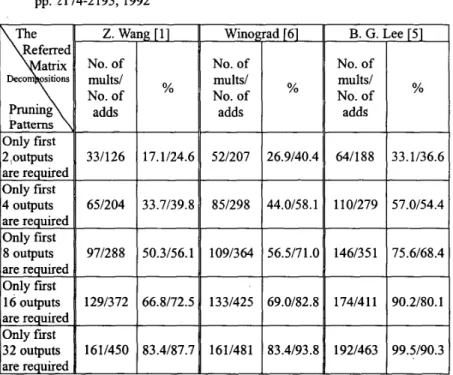
algorithm to derive efficient pruning DCT algorithms, based on the matrix decompositions presented in [1,5,6]. For the 1-D DCT of length 64, table 1 listed the numbers of required multiplications and additions for the corresponding pruning DCT algorithms with respect to different pruning patterns. The percentages of the required multiplications and additions of the so-

obtained pruning algorithms to that the original (un-pruned) algorithms are also listed in table 1 (in the columns headed by the notation %), as an index for checking the effectiveness of each corresponding matrix decomposition, from the view point of output pruning.

The reason for choosing this special transform length comes from the fact that the numbers of required multiplications and additions for all the algorithms presented in [1,5,6] are the same and equal to 193 and 5 13, respectively.

The most well-known pruning DCT algorithm presented in [ 11 gives the same complexities as listed in the first column of table 1. This fact verifies the correctness and effectiveness of the proposed pruning algorithm. As for the other two algorithms (or matrix decompositions), the gain obtained from pruning is less significant. The number of pruned multiplications is larger in the Winograd’s approach, whereas the number of pruned additions is larger in the Lee’s approach. In fact, these characteristics can be observed and explained from their corresponding algorithm structures: In the Winograd’s DCT algorithm, the required multiplications are post-processing oriented; whereas, in the Lee’s DCT algorithm, the most post-processing oriented operations are additions. That is, if the complexity of multiplication is the major concern, then the pruning gain will be more significant when the required multiplications of the algorithm are nearly post-processing oriented.

V.

Conclusions

In this paper, the derivation of efficient pruning DCT algorithms is the major focus. Since the effectiveness of the proposed output pruning algorithm is matrix-decomposition-dependent, some existing well-known DCT and pruning DCT algorithms are examined. Simulation results show that the resultant pruning DCT algorithm, derived based on the proposed approach, and the matrix decomposition presented in [ 11 needs the same computational complexity as that of the best existing pruning DCT algorithm [ l ] does (for some regular pruning patterns). From the derivation presented in section 11, it follows that there is not any restriction on the pruning pattern for the proposed approach. In other words, the resultant pruning DCT algorithm can work as well as some well-known pruning algorithms, but it dispenses with the pruning pattern constraint that most of the other pruning approaches may have (such as the ones given in [ 1-31).

VI. References

[I]

[2]

ZhongDe Wang, “Pruning the Fast Discrete Cosine Transform,” IEEE Trans. on Communication vol. 39 no. 5, May, pp. 640-643, 1991

..

Athanassiou N. Skodras, “Fast Discrete Cosine Transform Pruning,”

IEEE Trans. on Signal processing, vol. 42, no. 7, July, pp. 1833-1837, 1994.

C. A. Chstopoulos, J. Bormans, J. Cornelis, A. N. Skodras, “The Vector- Radix Fast Cosine Transform : Pruning and Complexity Analysis,” Signal Processing, vol. 43, pp. 197-205, 1995.

Hsieh S. Hou, “A Fast Recursive Algorithm for Computing the Discrete Cosine Transform,” IEEE Trans. on Acoustics, Speech and Signal Processing, vol. Assp-35, no. 10, Oct. 10, pp. 1455-1461, 1987.

[5] B. G. Lee, “A New Algorithm to Compute the Discrete Cosine Transform,” IEEE Trans. on Acoustics, Speech and Signal Processing, vol. Assp-32, no. 6, pp. 1243-1245, 1984

Ephraim Feig, Shmuel Winograd, “Fast Algorithms for the Discrete Cosine Transfomi,” IEEE Trans. on Signal Processing, vol. 40, no.9, Sep., [3] [4] [6] pp. 2174-2193,1992 Z. Wang 111 E f e n e d aeix NO. of are required

1

Only first

I

32 outputs 1611450 83.4187.7 are required Winograd [61 B. G. Lee [5] No. of No. of multsl multsl No. of % No. of adds adds % 521207 26.9140.4 641188 33,1136.6

Table 1. The numbers of required multiplications and additions for the resultant pruning DCT algorithms with respect to different matrix decompositions and different pruning patterns.