An Effective Dynamic Task Scheduling Algorithm for Real-time Heterogeneous Multiprocessor Systems

全文

(1)An Effective Dynamic Task Scheduling Algorithm for Real-time Heterogeneous Multiprocessor Systems Wen-Pin Liu, Yi-Hsuan Lee, and Cheng Chen* Department of Computer Science and Information Engineering National Chiao-Tung University 1001 Ta Hsueh Road, Hsinchu, Taiwan, 300, Republic of China E-mail: {wpliu, yslee, cchen}@csie.nctu.edu.tw Multiprocessor systems have emerged as a powerful. Abstract Real-time systems require both functionally correct. computing means because of their capability for high. executions and the results that are produced in time.. performance and reliability for the real-time applications. Fault-tolerance is an important requirement of such. [8, 13-14]. Due to the nature of real-time tasks, several. systems, due to the catastrophic consequences of not. techniques have evolved for fault-tolerant scheduling [2, 4,. tolerating faults. In this paper, we propose an effective. 10]. In multiprocessor systems, fault-tolerance can be. Load-driven Adaptive Scheduling Algorithm (LASA) to. provided by scheduling multiple versions of tasks on. dynamically schedule real-time tasks with fault-tolerance. different processors. Among different schemes for. used in heterogeneous multiprocessor systems. In LASA, it. fault-tolerant scheduling, we choose the Primary/Backup. has an adaptive mechanism to monitor the processor. (PB) scheme which is the most popular one.. utilization and determine the number of backup copies. In recent years, the adaptation mechanism opens up. been scheduled. Besides, we also design a task deferment. many avenues for further research in the dynamic. mechanism to improve the utilization of reclaimed. scheduling problem [14]. The concept of adaptation. computing resources from redundant copies. According to. mechanism is to allow the scheduler dynamically adjust. our simulations, LASA makes a trade-off between the. its scheduling strategy, which can flexibly satisfy the. guarantee ratio and the reliability of fault-tolerance, and. different requirements under different circumstances. In. obviously outperforms other related methods.. this. Keywords: Heterogeneous multiprocessor, Real-time,. Scheduling Algorithm (LASA), which will adjust the. Task scheduling, Adaptive, Fault-tolerant. number of backup copies been scheduled based on current. paper,. processor. we. propose. utilization.. Loading-driven. Clearly,. Adaptive. LASA introduces. a. Introduction. trade-off between rejecting fewer tasks and risking the. Real-time systems are defined as those systems in. fault-tolerance. Besides, we add a waiting queue to collect. which the correctness of the system depends not only on. unschedulable tasks instead of directly reject them. When. the logical result of computation, but also on the time at. the computing resources are reclaimed after deallocating. which the results are produced [1]. In such systems, the. backup copies, tasks in the waiting queue can be. real-time task scheduling can be performed either. rescheduled to improve the overall schedulability. From. statically or dynamically. Since there does not exist an. the simulation results, our LASA outperforms other. optimal scheduling algorithm for dynamically arrival. related algorithms.. 1. The remainder of this paper is organized as follows.. tasks, many heuristic approaches have been evolved [1, 4, 8, 11-12].. Section 2 describes the system model and related work. 1.

(2) Design issues and principles of LASA are introduced in. LFP(Ti) = di – min{cij}, ∀ Pj. section 3. In section 4, some performance evaluations are. Definition 2.2 For a task Ti, EFTj(Ti) indicates its Earliest. given. Finally, we give some conclusions in section 5.. Finish Time on Pj. If Ti cannot be completed before di on Pj, EFTj(Ti) is set as infinite.. 2 2.1. Definition 2.3 For a task Ti, its Earliest Finish Time (EFT). Fundamental Background. is defined as. System, Task, and Fault Models. EFT(Ti) = min{EFTj(Ti)}, ∀ Pj. The heterogeneous multiprocessor system consists of m application processors P1…Pm connected by a network. Definition 2.4 For a task Ti, its Latest Start Time of. and one dedicated scheduler. The communication. primary (LST) is defined as LST(Ti) = di – max{cij} – 2ndmax{cij}, ∀ Pj. between the scheduler and application processors is through dispatch queues. Real-time tasks arrive at the. Definition 2.5 H(Ti) is the heuristic function defined as H(Ti) = EFT(Ti) + di, if EFT(Ti) is not infinite. scheduler and executed separately on all application processors. The Spring system is such an example [3].. Definition 2.6 For a task Ti, BLSTj(Ti) indicates its Latest Start Time of backup on Pj. If Bki cannot be completed. Because [17] have proven that precedence constraints can be actually removed, real-time tasks are usually. before di on Pj, BLSTj(Ti) is set as zero.. assumed non-preemptive, non-parallelizable, aperiodic,. Definition 2.7 For a task Ti, its Latest Start Time of. and independent [1, 4, 8, 11-15]. Every task Ti has. backup (BLST) is defined as BLST(Ti) = max{BLSTj(Ti)}, ∀ Pj except the one. following attributes: arrival time (ai), deadline (di), and. that executes Pri. computation time on processor Pj (cij) [11-12]. These attributes are not known a priori until Ti arrives at the. 2.3. Related Work. system. Each task Ti has primary (Pri) and backup (Bki). Because PB scheme schedules two copies of each. copies with identical attributes. Since tasks are not. task on different processors, the entire schedulability is. parallelizable, di – ri should be long enough to schedule. obviously. both primary and backup copies of Ti [4, 8].. BB-overloading and backup deallocation are designed to. decreased.. Therefore,. two. techniques. Assume that each task encounters at most one failure. reduce the negative influence [4]. Guarantee Ratio (GR),. either due to processor or software. That is, if Pri fails, Bki. which means the percentage of tasks whose deadlines are. will always be completed successfully. This also implies. met, is a common objective for real-time task scheduling. that there is at most one failure in the system at a time.. algorithms. In this paper we use the same definition of GR. The faults are independent, and can be transient or. as in [5, 11-14].. permanent. Simply, we assume the scheduler is fault free.. GR =. 2.2. Basic Terminologies [11, 12]. number of tasks whose deadlines are met × 100% total number of tasks arrived in the system. In the following, we list some definitions which will. Distance Myopic Algorithm (DMA) is a heuristic. be used in our proposed algorithm. For each task Ti, we. search algorithm that schedules real-time tasks on. don’t allow its two copies Pri and Bki been scheduled at. homogeneous multiprocessor with fault-tolerance [5, 11].. overlapped time intervals. In addition, Pri and Bki must be. It uses an integrated heuristic function to prioritize tasks,. executed on different application processors to tolerant. and a feasibility check window to achieve look-ahead. permanent processor failure.. nature. Fault Tolerant Myopic Algorithm (FTMA) is. Definition 2.1 For a task Ti, its Latest Finish time of. extended from DMA to be used on heterogeneous. Primary (LFP) is defined as. multiprocessor [11]. It further changes the mechanism of 2.

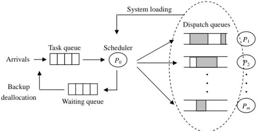
(3) System loading Dispatch queues P1 Task queue. Scheduler. Arrivals. Backup deallocation. P0. P2. • • • Waiting queue. • • • Pm. Figure 1. The loading-driven scheduler. task queue construction to improve the schedulability.. 3. Loading-driven Adaptive Scheduling Algorithm. Density first with minimum Non-overlap scheduling. (LASA). Algorithm (DNA) is another effective algorithm [12]. It. In Section 3.1, we give an overview of our proposed. proposes the density function to select the most urgent. Loading-driven Adaptive Scheduling Algorithm (LASA).. task, and the Minimum Non-Overlap (MNO) strategy to. Two main mechanisms of LASA, including the action of. minimize the reserved time slots for backup copies. All. waiting queue and the loading-driven adaptation strategy,. these three scheduling algorithms are quite efficient but. are described in Section 3.2 and 3.3 respectively.. never consider the adaptation mechanism.. 3.1. Overview. In the following we introduce two adapted scheduling. Before introducing proposed algorithm, we introduce. algorithms. [13] is an algorithm that can adjust the. the system model as shown in Figure 1. This architecture. number of copies of each task been scheduled. Each task. is similar as Spring system [3], with an additional waiting. is given the redundancy level and fault probability, where. queue and the feedback from dispatch queues to scheduler.. the redundancy level is the maximum number of copies it. Unschedulable tasks will be collected in the waiting. can be scheduled. A task contributes a positive value to. queue and tried to be rescheduled later, where other. the Performance Index (PI) if completed successfully.. related methods usually reject them directly. The. Conversely, it incurs a small PI penalty if rejected and a. information of system loading will be responded back to. large PI penalty if all its copies are failed. By evaluating. the scheduler. According to this feedback, the scheduler. the expected value of PI, the scheduler will decide the. will decide the backup copy of a task should be scheduled. number of copies that each task must be scheduled.. or not. Both these two mechanisms will be introduced in. [14] is a feedback-based algorithm that can adjust the. detail later.. degree of overlapping between the primary and backup. Our proposed LASA mainly contains three phases: to. copies of the same task. Its adapting strategy is based on. select a task from the task queue, to allocate the selected. an estimation of the primary fault probability and laxities. task to application processors, and to reject unfitted tasks. of tasks. However, this algorithm is impractical because. from the waiting queue. In this subsection we describe the. to decide the degree of overlapping is difficult. Besides,. task selection and allocation without adaptation strategy.. backup deallocation technique is unfit for this algorithm,. The action of waiting queue and adaptation strategy will. because only part of backup copies is reclaimed.. be introduced in Section 3.2 and 3.3. 3.

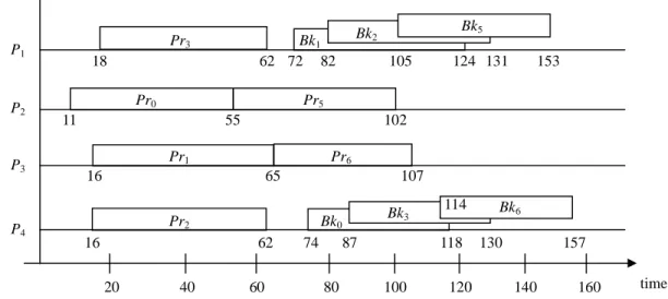
(4) Pr3. P1. 18 Pr0. P2. 55 Pr1. 153. Pr6 65. 107. Pr2. Bk3. Bk0. 16. 62 20. 124 131. 102. 16. P4. 105. Pr5. 11. P3. Bk5. Bk2. Bk1 62 72 82. 40. 74. 60. 87 80. 114 118. 100. 120. Bk6 130. 157 140. 160. time. Figure 3. The complete scheduling result of task set in Figure 2.. T0. T1. T2. T3. T4. T5. T6. T7. T8. T9. use ASAP and ALAP strategies to schedule Pri and Bki. ri. 11. 16. 16. 18. 29. 45. 48. 53. 54. 70. respectively in LASA. In order to increase the overall. di. 118 124 131 130 137 153 157 173 165 165. schedulability, BB-overloading technique is also applied.. ci1. 52. 52. 49. 44. 46. 48. 53. 45. 43. 47. The first two phases of LASA will be executed repeatedly. ci2. 44. 52. 54. 48. 47. 47. 52. 54. 45. 46. ci3. 53. 49. 56. 56. 58. 48. 42. 57. 48. 46. ci4. 44. 53. 46. 43. 44. 43. 43. 59. 46. 44. until the task queue is empty. For example, Figure 2 lists a task set and its attributes. Suppose there are four application processors, the complete scheduling result of this task set is shown in. Figure 2. A task set and its attributes.. Figure 3. From this result, we can find that tasks T4, T7, T8,. In the first phase, the heuristic values H(Ti) of all. and T9 are moved into the waiting queue and the GR. tasks in the task queue are calculated based on Definition. equals to 60%.. 2.5. During the calculation, if we find a task Ti with. 3.2. Task Deferment and Rejection in Waiting Queue. infinite EFT(Ti), which means Ti cannot be successfully. From related works we have surveyed, a task has only. scheduled currently, this task will be moved into the. one chance to be scheduled. If it cannot be successfully. waiting queue. After that, Ti with smallest H(Ti) value is. scheduled at that time, it will be rejected directly. In fact,. selected to be scheduled.. because Bki will be executed only when the corresponding. In the second phase, we try to schedule both primary. Pri fails, a task still has other chances to be rescheduled.. and backup copies of Ti to application processors. Notice. This situation is more obvious when the backup. that from the definition of EFT(Ti), only one task copy of. deallocation technique is applied. Therefore, in LASA,. Ti is considered. That is, for the selected task Ti, Pri can. we add a waiting queue to collect unschedulable tasks and. always be successfully scheduled but Bki may not.. try to reschedule them when every backup copy is. Therefore, we first calculate BLST(Ti) defined above. deallocated.. before scheduling Ti. If BLST(Ti) equals to zero, Ti is. Meanwhile, we also need a mechanism to reject. moved to the waiting queue because there is no available. unfitted tasks from the waiting queue that cannot be. time slot for Bki on any application processor. Otherwise,. successfully rescheduled any more. Hence, before. both Pri and Bki can be successfully scheduled. We simply. rescheduling, we calculate LST(Ti) values of tasks in the 4.

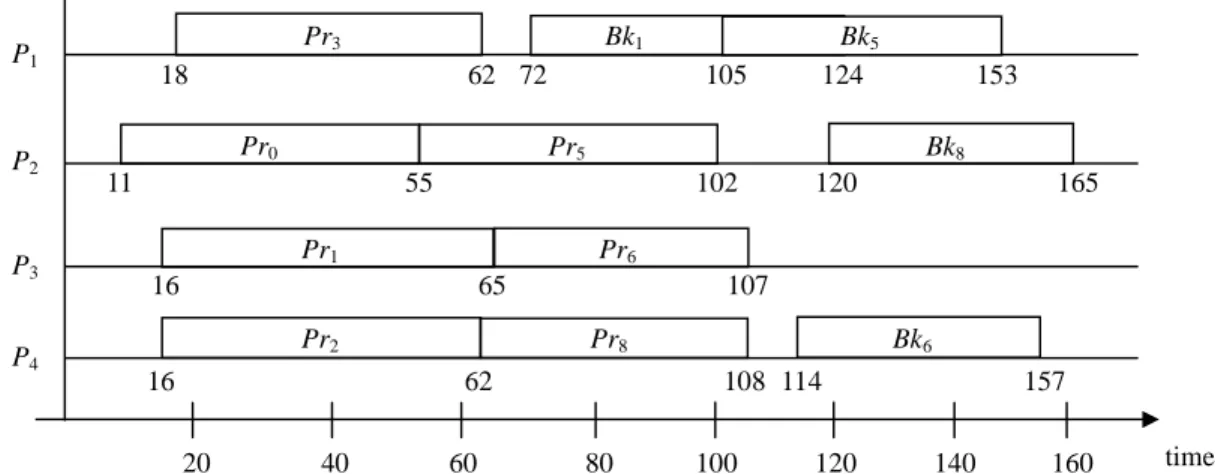
(5) Pr3. P1. P2. P3 P4. Bk1. 18. 62 72 Pr0. 105. Bk5 124. 153. Pr5. 11. Bk8. 55. 102. Pr1 65. 107. Pr2. Pr8. Bk6. 62 20. 40. 165. Pr6. 16. 16. 120. 108 114. 60. 80. 100. 157. 120. 140. 160. time. Figure 4. The scheduling result of task set in Figure 2 (with the waiting queue). Accept Ti Allocate Pri and Bki. Accept Ti Allocate Pri only. 3.3. When too many tasks arrive at a small time interval,. L. the system is overloaded and some tasks will be rejected. LA EFT(Ti) ≠ ∞. Loading-driven Adaptation Strategy. BLST(Ti) ≠ 0. by the scheduler. Since rejecting tasks degrades the overall GR (or schedulability), it is reasonable to. Move Ti into the waiting queue. Accept Ti Allocate Pri only. intentionally stop scheduling backup copies to accept more tasks. This approach apparently takes a trade-off. L. LR EFT(Ti) ≠ ∞. between the GR and the degree of reliability. Hence, in. BLST(Ti) = 0. LASA, we propose a loading-driven adaptation strategy, which aims to improve the GR without sacrificing too. Figure 5. Adaptation strategy used in LASA.. much reliability. waiting queue. All LST(Ti) values are compared with the. Definition 3.1 For a real-time system with m application. time that the backup deallocation just happens. If any. processors, L denotes the system loading defined as:. LST(Ti) is smaller, which means Ti has missed the latest. L=. time been successfully scheduled already, that task will be rejected from the waiting queue.. 1 avg (cij ) , ∑ m i di − ai. for all tasks currently resided in dispatched queues. Let us consider the previous example. Suppose no. and avg(cij) indicates the average execution time of Ti on P1…Pm. failure happens, Bk0 will be deallocated at time 55. At that time, three tasks T4, T7, and T8 in the waiting queue are. As shown in above definition, we use the processor. with LST(Ti) values 32, 57, and 63 respectively. Clearly. utilization in a small time interval to indicate the system. that T4 is rejected. Because both T7 and T8 cannot be. loading. L is dynamically calculated by the scheduler. In. rescheduled at that time, they are resided in the waiting. the beginning, all dispatch queues are empty and L equals. queue. Then, at time 62, Bk2 and Bk3 are deallocated. to zero. Then, L increases when the scheduler dispatches a. simultaneously. At this time, T7 is rejected and T8 is. new task, and decreases when a dispatched task is. successfully rescheduled on P4 and P2. The modified. finished either successfully or faultily.. scheduling result is shown in Figure 4. We can see that. Our adaptation strategy is appended to the task. GR is improved from 60% to 70%.. allocation phase in LASA. Two thresholds LA and LR are 5.

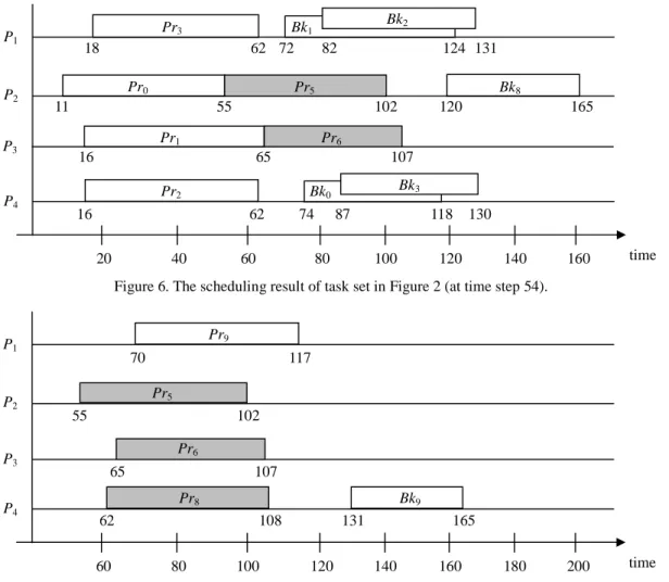
(6) Pr3. P1. P2 P3. P4. Bk2. Bk1 62 72 82. 18 Pr0. 124 131. Pr5. 11. Bk8. 55. 102. Pr1. 165. Pr6. 16. 65 Pr2. 107 Bk3. Bk0. 16. 62 20. 120. 40. 74. 60. 87 80. 118 100. 130. 120. 140. 160. time. 200. time. Figure 6. The scheduling result of task set in Figure 2 (at time step 54). Pr9. P1. P2. P3 P4. 70. 117 Pr5. 55. 102 Pr6 65. 107 Pr8. 62 60. Bk9 108. 80. 100. 131 120. 165 140. 160. 180. Figure 7. The scheduling result of task set in Figure 2 (at time step 70). given in advance. As the variation of L, we adaptively. both two copies and T4 has been moved into the waiting. apply three mechanisms as follows to allocate the selected. queue. At that time, even through both feasible time slots. task Ti.. for Pr5 and Bk5 can be found, only Pr5 is allocated. Case 1: If both feasible time slots of Pri and Bki can be. because L = 0.451 > LA. Similarly, T6 is accepted with. found, Ti is accepted. Pri is allocated directly, but Bki is. only Pr6 been allocated. After the scheduler moves T7 and. only allocated if L ≤ LA.. T8 into the waiting queue, the partial scheduling result is. Case 2: If only the feasible time slot of Pri can be found,. shown in Figure 6 (time step 54).. Ti is accepted with condition L > LR. Otherwise, Ti is. At time step 55, the scheduler deallocates Bk0 and. moved to the waiting queue.. rejects T4. When Bk2 and Bk3 are both deallocated at time. Case 3: If the feasible time slot of Pri cannot be found, Ti. step 62, T7 is rejected and only Pr8 is allocated because L. is moved to the waiting queue directly.. = 0.448 > LA. Then, at time step 70, T9 is accepted with. Above allocation mechanisms are illustrated in Figure. both two copies because L becomes 0.319. Figure 7. 5. Notice that the quantitative relation between LA and LR. shows the complete scheduling result at time step 70. We. is uncertain. Considering the previous example, suppose. can see that with the loading-driven adaptation strategy,. that LA and LR equal to 0.4 and 0.5 respectively. When T5. GR is further improved to 80%. Finally, the overall. arrives at time step 45, T0~T3 have been scheduled with. algorithm of LASA is listed in Figure 8. 6.

(7) 1. Calculate H(Ti) for all tasks in the task queue. Parameter. if (EFT(Ti) is infinite) Move Ti into the waiting queue 2. Select Ti with the smallest H(Ti). Explanation. MIN_C. Min. execution time. 10. MAX_C. Max. execution time. 80. 3. Find feasible time slots for the selected Ti 4. if (BLST(Ti) is not zero). λ. Task arrival rate. R. Laxity. m. if (L > LA) Allocate only Pri else Allocate Pri and Bki. {0.4, 0.5, …, 1.2} {2, 3, …, 10}. Number of application processors. {3, 4, …, 10}. Figure 9. Parameters used in the task generator.. else if (L > LR) Allocate only Pri else Move Ti into the waiting queue. Parameter. 5. Repeat steps 1~4 until the task queue is empty 6. if backup deallocations happened at time step t. FP. Calculate LST(Ti) for all tasks in waiting queue if (LST(Ti) < t) Reject Ti. Probability of a primary copy [0, 0.1] failure Probability of software failure. 0.2. Probability of hardware failure. 0.8. Performance Evaluations MAX_Recovery. a simulation environment to evaluate it. Our environment. Values. SoftFP. PermHardFP. After designing the algorithm of LASA, we construct. Explanation. HardFP Figure 8. The overall algorithm of LASA. 4. Values. Probability of a permanent hardware failure Maximum recovery time after a transient hardware fault. 10-6 50. Figure 10. Parameters used in the dynamic simulator.. and experimental results are described in this section. 4.1. that processor will be available after MAX_Recovery.. Simulation Environment. Probabilities for failures and related parameters are listed. Our environment contains two parts named the task generator and the dynamic simulator. The task generator. in Figure 10 [12].. generates a real-time task set in the non-decreasing order. 4.2. Experimental Results. of arrival times. Figure 9 lists all used parameters, which. In this subsection, we evaluate performances of. can generate task set with any characteristic [12]. For a. FTMA, DNA, n_DNA (DNA with waiting queue), LASA,. task Ti, its worst case execution times cij are uniformly. and m_LASA (LASA with MNO strategy). For each set. distributed in interval [MIN_C, MAX_C]. The inter-arrival. of parameters, we generate 20 task sets and each one. times between tasks is exponentially distributed with. contains 20000 independent tasks. Moreover, because. mean (MIN_C + MAX_C) / 2λm [5]. In order to make sure. FTMA requires additional parameters, we evaluate it with. that both copies of Ti can be successfully scheduled, its. various parameter combinations and select the best result.. deadline di is chosen uniformly between (ai + max cij +. We directly use the GR defined above as the objective.. 2 max cij, ai + R × max cij). nd. Figures 11~13 shows the GR of different scheduling. The dynamic simulator simulates events including. algorithm with various task arrival rates (λ), task laxity. task arrivals, task finishes, backup deallocations, and. (R), and the number of processors (m). In these. failure occurs. We consider three failure types: software. evaluations we simply assume all application processors. failure, permanent hardware failure, and transient. are fault-free. Interestingly, results in these figures are. hardware failure. A software failure immediately. quite similar. FTMA has the lowest GR because it. terminates the task that causes the fault. The failed. schedules backup copies by ASAP strategy, which is hard. processor with permanent hardware failure will never be. to take advantages from backup deallocation. Next, DNA. available. Contrarily, if the hardware failure is transient,. performs better than that of FTMA, since it highly 7.

(8) 100%. 100%. 95%. 99% 98% Guarantee Ratio. Guarantee Ratio. 90% 85% 80% FTMA DNA n_DNA m_LASA LASA. 75% 70% 65%. 97% 96% 95% 94%. FTMA DNA n_DNA m_LASA LASA. 93% 92% 91%. 60%. 90% 0.4. 0.5. 0.6. 0.7 0.8 0.9 Task arrival rate. 1. 1.1. 2. 1.2. 3. 4. 5. 6 Laxity. 7. 8. 9. Figure 11. Effect of the task arrival rate (λ).. Figure 12. Effect of the laxity (R).. (R = 3, m = 8, FP = 0, LA = 0.95, LR = 1). (λ = 0.7, m = 8, FP = 0, LA = 0.95, LR = 1). 100%. 10. 100% 95%. 95% Guarantee Ratio. Guarantee Ratio. 90% 90% 85% FTMA DNA. 80%. n_DNA. 85% 80% 75% 70%. m_LASA. 75%. 4. 5 6 7 8 Number of processors. 9. (1.2, 8, 3) (0.7, 10, 3). 60% 0.01 0.02 0.03 0.04 0.05 0.06 0.07 0.08 0.09 0.1. 70% 3. (0.4, 8, 3) (0.7, 3, 3) (0.7, 8, 3). 65%. LASA 10. Failure Probability. Figure 13. Effect of the number of processors (m).. Figure 14. Effect of the failure probability.. (R = 3, λ = 0.7, FP = 0, LA = 0.95, LR = 1). The 3-tuple indicates (λ, m, R). and. workload is heavy. However, the decrease of GR is. deallocation. From performances of DNA and n_DNA,. actually not significant, which means the performance of. we find that adding the waiting queue can cause the. LASA is quite stable.. exploits. properties. of. backup. overloading. positive influence. In summary, LASA obviously has the. Next, in Figure 15, we evaluate the influence of GR. highest GR in most circumstances. According to curves of. between LA and LR. When LA varies from 0.5 to 1.0, the. LASA and m_LASA, we further conclude that MNO. decrease of GR is about 5% in different LR values.. strategy is unfit for LASA.. Contrarily, for any constant LA, the difference of GR is. Figure 14 shows the GR of our LASA with various. less than 0.5% when LR varies from 0.7 to 1.0. It is. failure probabilities (FP). We find that the GR decreases. obvious that the value of LA causes more influence of GR. with the FP increasing in all cases, especially when the. than that of LR. 8.

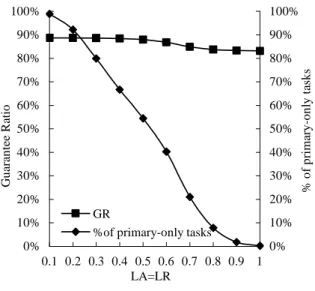
(9) 100%. LR=0.7. 90%. 90%. LR=0.8. 80%. 80%. LR=0.9. 70%. 70%. LR=1.0. 86%. 60%. 60%. 50%. 50%. 40%. 40%. 30%. 30%. Guarantee Ratio. Guarantee Ratio. 87%. 85%. 20%. 84%. 20% GR %of primary-only tasks. 10%. 10%. 0%. 83% 0.5. 0.6. 0.7. 0.8. 0.9. % of primary-only tasks. 100%. 88%. 0% 0.1 0.2 0.3 0.4 0.5 0.6 0.7 0.8 0.9 1 LA=LR. 1. LA. Figure 15. Effect of the threshold values.. Figure 16. Effect of the threshold values.. (R = 3, m = 8, λ = 1.2, FP = 0). (R = 3, m = 8, λ = 1.2, FP = 0). Finally, Figure 16 simultaneously shows the GR and. actually can improve the overall schedulability. Besides,. the percentage of primary-only tasks been scheduled with. although the system cannot tolerant failures when it is. various LA. Since the value of LR has slightly effects of. overloaded, the sacrifice of reliability is quite minor.. GR, we set LR equals to LA for convenience in this evaluation. In this figure, we find that when LA varies. References. from 1.0 to 0.1, the proportion of scheduled primary-only. [1] K. Ramamritham, J. A. Stankovic, and Perng-fei “Efficient. tasks increases from 0 to 100% but the improvement of. Shiah,. GR is less than 8%. Actually, the proportion of scheduled. Real-time. primary-only tasks can imply the fault-tolerant capability. Transactions on Parallel and Distributed Systems,. of the system. Therefore, if we don’t want to sacrifice too. Vol. 1, No. 2, pp 184-194, April 1990.. Scheduling. Multiprocessor. Algorithms Systems”,. for IEEE. [2] K. G. Shin and P. Ramanathan, “Real-Time. much reliability, LA should be set larger.. Computing: A New Discipline of Computer Science 5. Conclusions. and Engineering”, Proc. of IEEE, Vol. 82, No. 1, pp. In this paper, we propose an effective Loading-driven. 6-24, Jan. 1994.. Adaptive Scheduling Algorithm (LASA) to dynamically. [3] J. A. Stankovic, K. Ramamritham, “The Spring. schedule real-time tasks with fault-tolerance. LASA. Kernel: A New Paradigm for Real-Time Systems”,. mainly contains two features. First, an additional waiting. IEEE Transactions on Software Engineering, Vol. 8,. queue is added to collect unschedulabe tasks instead of. Issue 3, pp 62-72, May 1991.. [4] S.. reject them directly. These tasks are tried to be. Ghosh,. R.. Melhem,. and. D.. Mosse,. rescheduled at proper time. Second, based on the. “Fault-Tolerance Through Scheduling of Aperiodic. information of system loading responded back to the. Tasks in Hard Real-Time Multiprocessor Systems”,. scheduler, we intentionally schedule only one copy of a. IEEE Transactions on Parallel and Distributed. task to accept more tasks when the system is overloaded.. Systems, Vol. 8, No. 3, pp 272-284, March 1997.. A simulation environment is also constructed to evaluate. [5] G. Manimaran and C. S. R. Murthy, “A. LASA. From experimental results, these two features. Fault-Tolerant Dynamic Scheduling Algorithm for 9.

(10) Multiprocessor. Real-Time. Systems. and. Its. 64, No. 5, pp 629-648, May 2004.. Analysis”, IEEE Transactions on Parallel and. [14] R. Al-Omari, A. K. Somani, and G. Manimaran, ”An. Distributed Systems, Vol. 9, No. 11, pp 1137-1152,. Adaptive Scheme for Fault-Tolerant Scheduling of. Nov. 1998.. Soft Real- Time Tasks in Multiprocessor Systems”,. [6] R. Al-Omari, G. Manimaran, and A. K. Somani, “An. Proc.. Fault-tolerant. Parallel. and. Workshop on Real-Time Computing Systems and Applications, pp 197-202, 1995.. for. Improving. Multiprocessor. Real-time. [16] M. L. Dertouzos and A. K. Mok, “Multiprocessor. systems”, Proc. of International Parallel and. On-Line Scheduling of Hard Real-Time Tasks”,. Distributed Processing Symposium, April 2001.. IEEE Transactions on Software Engineering, Vol.. Schedulability. in. Technique. High. Multiprocessor Systems”, Proc. of International. [7] R. Al-Omari, A. K. Somani, and G. Manimaran, “A Fault-tolerant. on. Fault-Tolerant Scheduling Technique for Real-Time. Distributed Systems, pp 1291-1295, 2000.. New. Conference. [15] T. Tsuchiya, Y. Kakuda, and T. Kikuno, ”A New. Scheduling of Real-time Tasks”, Proc. of IEEE on. International. Performance Computing, Dec. 2001.. Efficient Backup-overloading for Fault-tolerant. Workshop. of. [8] R. Al-Omari, A. K. Somani, and G. Manimaran, “Efficient. Overloading. Techniques. 15, No. 12, pp1479-1506, Dec. 1989.. [17] J. W. S. Liu, W. K. Shih, K. J. Lin, R. Bettati, and J.. for. Primary-Backup Scheduling in Real-Time Systems”,. Y. Chung, “Imprecise Computations”, Proc. of IEEE,. Journal of Parallel and Distributed Computing, Vol.. Vol. 82, No. 1, pp. 83-94, Jan. 1994.. 64, No. 1, pp 629-648, Jan. 2004.. [9] C. Shen , K. Ramamritham , and J. A. Stankovic, “Resource. Reclaiming. in. Multi-. processor. Real-Time Systems”, IEEE Transactions on Parallel and Distributed Systems, Vol. 4, No. 4, pp 382-397, April 1993.. [10] L. V. Mancini, “Modular Redundancy in a Message Passing System”, IEEE Transactions on Software Engineering, Vol.12, No. 1, pp 79-86, Jan. 1986.. [11] Y. H. Lee, M. D. Chang, and C. Chen, “Effective Fault-tolerant Scheduling Algorithms for Real-time Tasks. on Heterogeneous Systems”, Proc. of. National Computer Symposium, Dec. 2003.. [12] M.. D.. Chang,. A. Fault-tolerant. Dynamic. Scheduling Algorithm for Real-time Systems on Heterogeneous Multiprocessor, Master Thesis, National Chiao-Tung University, June 2004.. [13] S. Swaminathan and G. Manimaran, ”A Value-based Scheduler. Capturing. Schedulability. Reliability. Tradeoff in Multi- processor Read-time Systems”, Journal of Parallel and Distributed Computing, Vol. 10.

(11)