Event-driven dynamic workload scaling for uniprocessor real-time embedded systems

Event-Driven Dynamic Workload Scaling

for Uniprocessor Real-Time Embedded Systems

LI-PIN CHANGAND YA-SHU CHEN+

Department of Computer Science National Chiao Tung University

Hsinchu, 300 Taiwan

+_{Department of Electrical Engineering} National Taiwan University of Science and Technology

Taipei, 106 Taiwan

Many embedded systems are designed to take timely reactions to the occurrences of particular scenarios. Such systems could sometimes experience transient overloads be-cause of workload bursts or hardware malfunctions. Thus a mechanism to focus limited resources on the processing of urgent events is a key to retain system validity under stressing workloads. In this paper, we propose a new approach for workload scaling in uniprocessor real-time embedded systems. The idea is to view the system as a black box, and workload scaling for overload management can be done via very intuitive primitives, i.e., how hardware events are selectively fed into the system. Such a new approach re-moves the need for the adjustments of task periods and task phasing, which is important for many workload-scaling techniques. The proposed approach is implemented in a real-time surveillance system. Experimental results show that the system still delivers good accuracy and high responsiveness for visual-object tracking under the presence of overloads.

Keywords: embedded systems, real-time systems, adaptive applications, overload

man-agement, real-time surveillance

1. INTRODUCTION

Many embedded systems are designed to take timely reactions to the occurrences of particular scenarios. For example, an automobile controlling system should simulta- neously control cruising, traction, the brake system, and the engine. A real-time sur- veillance system in a shopping mall could track a number of moving people and evaluate pre-defined rules to detect thieving. These systems might sometimes experience transient workload bursts due to hardware malfunctions (e.g., one processor fails in a dual- processor system) or workload bursts (e.g., a number of people suddenly rush into monitored areas). To prevent the systems from being overloaded, the system could smartly allocate available computing power among tasks so as to pay more attention to those urgent events and, at the same time, to slow down the processing of inactive events.

Consider an embedded system which deals with periodically recurring external (hardware) events. Intuitively, proportional period adjustment for periodic tasks could be

Received November 15, 2006; accepted February 15, 2007. Communicated by Sung Shin and Tei-Wei Kuo.

* _{This work was partly supported by the National Science Council of Taiwan, R.O.C., under grant No.}

useful to slow down or to speed up the processing of events. However, this simple approach has some major drawbacks: First, even though the period of a task could be arbitrarily adjusted, the recurring rate of a hardware event are usually not. Consider a thermal sensor connected to a system via USB and its reading is sampled every 1 ms. Because the minimal time frame for USB bus traffic is 1 ms, change the sampling rate to 1.5 ms is unlikely applicable. Second, mismatches of hardware-event recurring periods and task periods could sometimes result in unpredictable arrivals of events due to buffer overflows. Not being aware of which event is sampled and when it is sampled could damage the usefulness of timing-sensitive algorithms such as Kalman filters. Third, responsiveness for detecting pre-defined scenarios would largly be retarded due to long propagation delays introduced by improper task periods and task phasing. All these drawbacks of proportional period adjustment will be shown in our experiments.

B

B

lack box

lack box

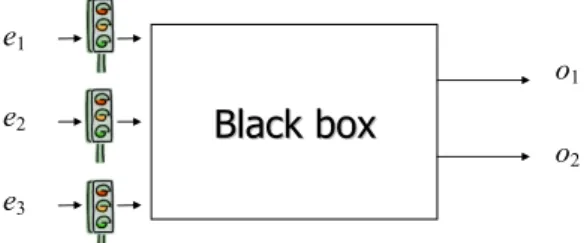
Fig. 1. A “black box” that receives periodic hardware events and then delivers outputs. In this paper, we propose a new approach for workload scaling in uniprocessor real-time embedded systems. Let a system be viewed as a “black box” (as shown in Fig. 1), and the system requires no intervention when workload scaling is conducted. When transient overloads are experienced, the feeding of events (i.e., e1, e2, and e3 in Fig. 1) could be controlled by some mechanism (i.e., the traffic lights in Fig. 1) to protect the system against timing violations. Our objectives are summarized as follows: (1) System workloads should be adjusted by means of very simple and intuitive primitives. (2) Tasks in the system should automatically react to new settings for workload scaling without intervention from the scheduler. (3) Tasks in the system should have deterministic timing behaviors. (4) An on-line admission control policy is needed to examine whether any change to system workloads can be made.

The rest of this paper is organized as follows: Section 2 provides past work related to the issues we considered. The system model and terminologies are introduced in sec-tion 3. System timing analysis and an efficient on-line admission control algorithm are presented in section 4. Performance evaluation and comparison are provided in section 5, and this paper is concluded in section 6.

2. RELATED WORK

As modern embedded software is component-based, event-driven paradigms are one of many software architectures to formulate precedence constraints among components. Tindell [13] considered an iterative approach to calculate response time for distributed

o1 o2 e1

e2 e3

event-driven tasks. The proposed analysis was extended to handle complex precedence constraints in hard-real-time distributed systems [14]. The model is applicable to many types of applications such as parallel and distributed systems [15] and embedded systems [16]. Precedence constraints among tasks could also be formulated as producer-consumer relation in uniprocessor systems [1]. Recently, operating systems based on event-driven models are also considered in the implementation of sensor nodes [8].

Dynamic workloads could transiently overload a real-time system. Prior work pro-posed many excellent workload-scaling approaches for overload management: In par-ticular, Koren and Shasha [4] proposed to schedule tasks while task jobs could be skipped in a controllable way. Hamdaoui and Ramanathan [5, 6] proposed the (m, k)-firm task model to complete at least m task jobs out of any k consecutive ones. Window- constrained scheduling [2, 3] is to fulfill m task jobs out of every window of k successive task jobs, while windows do not overlap one another. Imprecise computation [9] defines that any job is of a mandatory portion and an optional portion. Mandatory portions must be successfully completed before their deadlines, while the more CPU execution are contributed to optional portions the more reward is attained. Besides to skip jobs, task-period adjustment is also a commonly adopted technique [17, 18].

Besides considering new task models, an alternative approach for overload handling is to consider how “fresh” a piece of data is. Data freshness can be defined over time domain or value domain: A piece of fresh data stands for either one that has just been recently updated, or one which’s value has not been changed a lot. When systems are overloaded, either the sampling rates of those inactive events could be decreased [20], or only updates (i.e., jobs) to those “stale” data should be scheduled for execution [19]. However, there is no direct mapping from the definition of data freshness into how workload is scaled down. The algorithm may need to try a number of different settings before the system gets rid of being overloaded.

Different from prior work, this paper aims at a new approach for dynamic workload scaling. It employs no adjustment and alignment of task periods. With a proposed on-line admission control policy, workload adjustment can be done on the fly.

3. THE SYSTEM MODEL

Let tasks be preemptively scheduled with fixed priorities over a single processor. An event-driven task δi is a template of jobs, and job δi,n stands for the nth task job. Let each job of task δi require ci units of processor time, and a static priority Ωi be assigned to all jobs of task δi. A result is a piece of data that a task job prepares for another task, and an event is sent to the destination task when a predefined number of results are ready. A task job is released and becomes ready when the task receives an event. A task could either (1) receive one (and only one) hardware event, or (2) receive one or many events from other tasks. An event sent from task δi to task δj is denoted by ei,j, and a hardware event that task τi receives is denoted by e0,i. No tasks could receive both hardware events and events from other tasks. Let all hardware events be periodic, and pi stands for the recurring period of hardware event e0,i.

If δi sends events to task δj, then δi and δj are referred to as the producer and the consumer of each other. The relation is denoted by δi p δj. An event ei,j is composed by

ri,j cumulated results (ri,j ∈ Z+_{). Upon every ri,jth result is ready, δi composes an event} and sent to consumer δj. At the same time, a ready job of consumer δj is released. For any n ∈ Z+_{, job δ}

i,n⋅ri,j is referred to as an effective job of δi p δj since it triggers the execution of job δj,n. Note that each arrival of hardware event e0,j triggers the execution of a job of task δj because r0,j = 1.

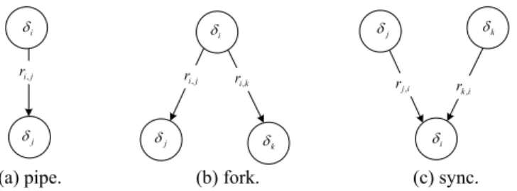
Task jobs are assigned to no explicit deadlines. Instead, a task job must complete before the next task job arrives. A task is referred to as a pump if it receives a hardware event. A taskchain Δ = {δ1, δ2, …, δn} is a collection of tasks, in which δ1 is a pump and δi p δi+1 for any {δi, δi+1} ⊆ Δ. As shown in Fig. 2, three basic structures are considered: pipes, forks, and syncs. Note that, in a sync, a consumer job becomes ready as long as the consumer receives at least one event from each producer of the sync.

j δ δ_k i δ j i r_, r_i,_k j i r_, i j r, rk,i j δ i δ δ_j δk i δ (a) pipe. (b) fork. (c) sync.

Fig. 2. Three basic structures in our event-driven system model.

For comparison and later use in this paper, a time-driven periodic system is defined as follows: A periodic task τi = (oi, ci, pi) is a template of jobs, and job τi,n denotes the nth task job. The first job of τi arrives at time oi and then a job arrives every pi units of time. In other words, job τi,m is released at time oi + (m − 1)pi for m ∈ Z+_{. Computation} re-quirement of each job of task τi is no more than ci units of time, and the relative deadline of a task job is the task period. A fixed priority Ωi is assigned to all jobs of task τi for preemptive scheduling.

4. WORKLOAD SCALING FOR EVENT-DRIVEN SYSTEMS

4.1 Timing Analysis for Pipes and Forks

This section aims at timing analysis of tasks in pipes and forks with or without event skips.

4.1.1 Scheduling without event skips

In pipes and forks, every consumer has only one producer. First we shall determine the optimal priority assignment for tasks in a taskchain:

Lemma 1 Given a taskchain Δ = {δ1, δ2, …, δn} and an arbitrary priority assignment A

= {Ω1, Ω2, …, Ωn}. If Δ is schedulable with A then Δ is also schedulable with a priority assignment A′ = {Ω1′, Ω2′, …, Ωn′}, in which Ω′i is higher than Ω′i+1 for any i.

Proof Sketch: It can be proved by repeatedly swapping priorities Ωi and Ωi+1 until Ωi is higher than Ωi+1 for any i. After each priority swap taskchain Δ is still schedulable. ‰ Under the optimal priority assignment, the following theorem shows that event- driven tasks in a taskchain can be equivalently modeled as a collection of independent periodic tasks in terms of timing behaviors:

Theorem 1 Given a taskchain Δ = {δ1, δ2, …, δn}. Let T be a set of independent peri-

odic tasks {τ1 = (0, c1, p1), τ2 = (p1(r1,2 − 1), c2, p1 ⋅ r1,2), …, τn = (p1 ⋅ (( ₁ 1, ) 1), n x x x=r− −

∏

c p ⋅

∏

Proof: We shall show the correctness of this theorem by induction on n the number of tasks:

I.B.: The base case is trivial.

I.H.: Suppose that the theorem is true when for n tasks.

I.S.: Consider the case {δ1, δ2, …, δn} ∪ {δn+1}. By I.H., δn is equivalent to a periodic task τ_n =(p₁⋅ ((

∏

∏

x

r₊ ⋅ ⋅p

∏

1 1, 1 ₁ 1,

1), _n , _{n n} n _{x x})

x

c₊ r₊ ⋅ ⋅p

∏

' 1 τ ' 2 τ ' 3 τ 1 δ 2 δ 3 δ

(a) Event-driven tasks. (b) Periodic tasks. Fig. 3. Modeling a collection of event-drive tasks as a collection of purely periodic tasks. Fig. 3 shows a schedule fragment resulted by three event-driven task Δ = {δ1, δ2, δ3}, where r1,2 = 2 and r2,3 = 1. Suppose c1 = 1, c2 = 2, and c3 = 2. The pump δ1 is driven by a hardware event e1 every 3 units of time. On the other hand, a collection of independent periodic tasks T = {τ1 = (0, 1, 3), τ2 = (3, 2, 6), τ3 = (3, 2, 6)} is considered. For all i, Ωi is assigned both to δi and to τi. Ω1 is the highest priority and Ω3 is the lowest priority. As shown in Fig. 3, Δ and T result in the same schedule, no matter how long the actual exe-cution times of jobs are.

Because a fork could be considered as a structure that “joins” one or more task-chains, Lemma 1 and Theorem 1 is still applicable to taskchains in a fork. Tasks in dif-ferent taskchains could be optimally assigned to priorities which are inversely propor-tional to the corresponding “periods” from Theorem 1.

4.1.2 Scheduling with event skips

With event skips, this section considers how tasks in pipes and forks behave. A firm-real-time scheduling technique is first introduced, and timing analysis is then pre-sented.

1. (m, k)-Firm Scheduling

We choose to adopt (m, k)-firm scheduling [5, 6] as the policy for event selection so as to achieve workload scaling. A (m, k)-firm task is a generalization of a periodic task. A task being subject to (m, k)-firm constraint must successfully complete m jobs before their relative deadlines (i.e., the period) out of any k consecutive jobs. A job is classified as being mandatory if it has to be completed in time, or it is classified as being optional. Let all jobs of a task be labeled with their ordinal numbers and the smallest number be zero. The following equation classifies which job should be classified as being man-datory: , . i m k _{i Z} k m ⎢ ⋅⎡ ⎤ ⎥ _∈ ⎢⎢_⎢ ⎥_⎥ ⎥ ⎣ ⎦ (1) For example, a task being subject to (3, 5)-firm constraint must successfully com-plete the jobs labeled with 0, 1, 3, and so on. An alternative form representing (m, k)-firm constraint is an array of k binary elements: A job labeled with i is a mandatory job if the i%kth element1 _{is 1, otherwise the job is an optional job. For example, (3, 5)-firm} con-straint can be represented as 11010. The array is referred to as the activation pattern of (3, 5)-firm constraint.

Derived from Eq. (1), two functions can be derived: (1) f(n) that calculates the smallest ordinal number of a job until which there are n jobs had been classified as being mandatory2, and (2) h(n) that calculates the number of jobs classified as being mandatory from the job labeled with zero to the job labeled with n:

( 1) ( 1) ( ) n k , and ( ) n m . f n h n m k − + ⋅ ⎢ ⎥ ⎡ ⎤ =_{⎢ ⎥} =_{⎢ ⎥} ⎣ ⎦ ⎢ ⎥ (2) 2. Scheduling Event-Driven Tasks with (m, k)-firm Constraint

When (m, k)-firm constraints are applied to pumps (i.e., tasks that receive hardware events) to skip some certain events, the question that what are the timing behaviors of consumer tasks behave in taskchains needs to be answered.

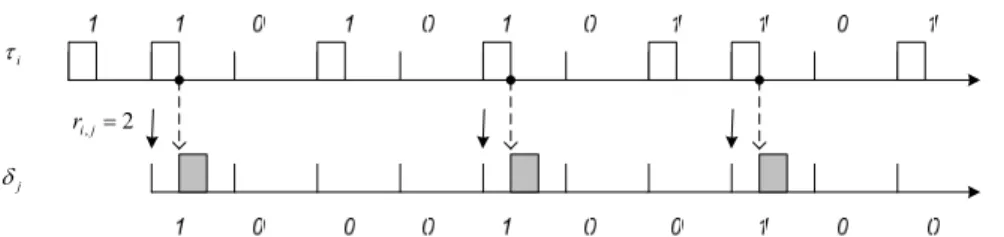
Consider the example shown in Fig. 4, where producer δi is subject to (4, 7)-firm

1 _{% is the modulus operator and the array elements are labeled from zero.} 2 _{f(n) is an abbreviation of} k_{( ).}

m

i τ j δ 2 ,j= i r

Fig. 4. A producer-consumer pair of task δi and task δj, where δi is a pump being subject to (4, 7)- firm constraint.

constraint. Based on the same arguments in the proving of Theorem 1, consumer δj could be treated as a periodic task which inherits task period pi from producer δi and is subject to an activation pattern {1000100}. It is conjectured that the pattern {1000100} is the result of rotating the activation pattern of (4/ri,j, 7)-firm (i.e., (2, 7)-firm) constraint by three elements leftward (i.e., {1001000} → {1000100}).

To verify our conjecture, the notion of pattern rotations is introduced: Let the acti-vation pattern of (m, k, ε)-firm constraint be the result of rotating the pattern of (m,

k)-firm constraint by ε elements leftward. Let us be focused on

(

)

(( 1) ) ( ) n k k . f n m m ρ ρ − + ⋅ ⎢ ⎥ ⎢ ⎥ ′ =_{⎢ ⎥ ⎢}− _⎥ ⎣ ⎦ ⎣ ⎦ (3) Consider δip δj, where δi is subject to (m, k)-firm constraint. Based on the same ar-guments in the proving of Theorem 1 and f() in Eq. (2), the arrival times of δj’s jobs are:

, , ( 1) ( 1) . i j i j r n k r k m m − − ⎢ ⎥ ⎢ ⎥ − ⎢ ⎥ ⎢ ⎥ ⎣ ⎦ ⎣ ⎦

Suppose that m = ri,j ⋅ m′ for some m′ ∈ Z. By some modulus algebra the above equation could be rewritten as

((n 1) ( 1))k ( 1)k m m π π − + + + ⎢ ⎥ ⎢₋ ⎥ ⎢ _′ ⎥ ⎢ _′ ⎥ ⎣ ⎦ ⎣ ⎦ (4) for some π ∈ Z. Comparing Eq. (3) with Eq. (4), obviously the consumer is subject to

(

)

m k′ ⎢_⎢ π +_′ ⎥_⎥

⎣ ⎦ constraint. Let a firm-real-time task τ is denoted by ((o, c, p), (m, k, ε)), where o, c, and p denote the initial arrival time, the computation demand, and the period of task τ respectively. τ is subject to (m, k, ε)-firm constraint. Now Theorem 1 can be generalized as follows:

Corollary 1 Given a taskchain Δ = {δ1, δ2, …, δn}, where pump δ1 is subjected to (m1,

k1, ε1)-firm constraint and ₁ 1, x

i i

i=r−

∏

1 1 1 1 1 1 1 1 1 1 1 1, 2 2 1 1 2 1, 2 1 1 ₁ 1, 1 1 1, 1 {((0, , ), ( , , )), (( ( ), , ), ( , , )), , (( ( ), , ), ( , , ))}. k m n k n m i i i n n n i i i m c p m k p f r c p k r m p f r c p k r ε ε τ _{= −} ε − = =

∏

∏

Systems Δ and T produce same schedule under a priority assignment in which Ωi is higher than Ωi+1 for any i.

Proof: It directly follows Theorem 1 and the above discussion. ‰

4.2 Timing Analysis for Syncs

Now let our attention be focused on timing analysis for tasks involved in sync struc-tures. As we did in the previous sections, the discussions first begin with scheduling event-driven tasks in syncs, where no event skips are allowed.

Let the consumer δc of a sync be an event-driven task, and the producers of the sync be independent periodic tasks. Let Aδc = {τi |τi p δc} be a collection of tasks including all producers of consumer δc. For any producer τ ∈ Aδc, the inter-arrival time of the effec-tive jobs of τ p δc is referred to as the effective cycle of producer τ. Consumer job δc,x becomes ready as soon as all effective jobs in {τi,x⋅ri,c |∀i : τi ∈ Aδc} send an event to

con-sumer δc. Priorities assigned to producers are inversely proportional to their recurring periods, and the consumer is assigned to the lowest priority (as shown in Lemma 1).

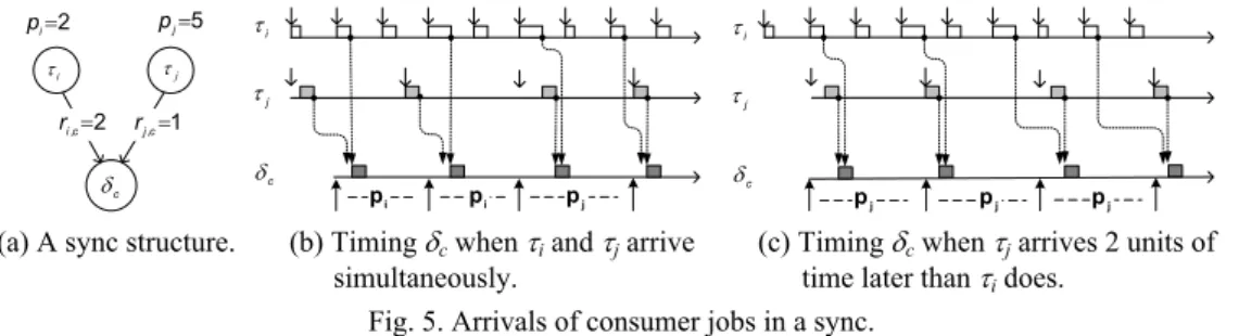
Fig. 5 depicts a scenario in which two periodic producers τi and τj conjunctively trigger the execution of the event-driven consumer δc. As Fig. 5 (b) shows, even though the producer τi and τj periodically issue events to consumer δc, jobs of δc do not arrive in a regular period. On the other hand, as Fig. 5 (c) shows, if the first effective job of τj (i.e., τj,1) arrives no earlier than the effective first job of τi (i.e., τi,2) does, then all jobs δc will be released every rj,c ⋅ pj units of time as if δc were a periodic task. The adjustments of task arrival times could be formulated as the following corollary:

j i τ τ c δ i τ τj c δ 2 ,c= i r rj,c=1 2 = i p pj=5 j i τ τ c δ i p pi pj pj pj pj

(a) A sync structure. (b) Timing δc when τi and τj arrive simultaneously.

(c) Timing δc when τj arrives 2 units of time later than τi does.

Fig. 5. Arrivals of consumer jobs in a sync.

Corollary 2 Suppose that task δc is conjunctively driven by events sent from a

collec-tion of independent periodic task Γ = Aδc. Let be

, , , , , { } : , ( 1) ( 1) . i j i i c i j c j i i c i j j c j r p r p o r p o r p τ τ τ ∃ ∈ Γ ∀ ∈ Γ − ⋅ ≥ ⋅ + − ≥ + −

Consider a periodic task τc = (oi + (ri,c − 1)pi, cc, ri,cpi). Systems Γ ∪ {τc} and Γ ∪ {δc} produce the same schedule.

Proof: For any job δc,x of task δc, the job becomes ready as soon as every task τj ∈ Γ

sends x events to task δc. Because the arrival of job τi,x⋅ri,c is always the latest among those

of jobs τj,x⋅ri,c and task δc is assigned to the lowest priority, the processor would not be

available to job δc,x until job τi,x⋅ri,c completes. Job δc,x could then be treated as one that

arrives simultaneously with job τi,x⋅ri,c, and the inter-arrival time of jobs of δc is pi⋅ ri,c.

Obviously, Γ ∪ {τc} and Γ ∪ {δc} produce the same schedule. ‰ A simple algorithm based on topological sort could be adopted to adjust pumps’ ini-tial arrival times to comply with the condition stated in Corollary 2. Corollary 2 can be revised accordingly to analyze tasks in sync with event skips.

4.3 On-Line Admission Control

As previous sections show, all event-driven tasks could be exactly modeled as in-dependent periodic tasks. This section is then focused on providing an efficient sched-ulability test for a collection of periodic tasks being subject to (m, k, ε)-firm tasks.

Let a periodic task being subject to (m, k, ε)-firm constraint be referred to as a (m, k, ε)-firm task for conciseness. Consider that a collection of event-driven tasks {δ1, δ2, …, δn} had been successfully modeled as a collection Tn of (m, k, ε)-firm tasks {τ1, τ2, …, τn}. The critical instance of T occurs when all (m, k, ε)-firm tasks are in phase and εi = 0 for all τ ∈ Tn. Because each task job must complete before the next task job arrives (please see section 3), the schedulability test based on worst-case response time analysis is as follows:

Lemma 2 [5] A collection of (m, k, ε)-firm tasks Tn = {τ1, τ2, …, τn} with arbitrary

arrival times is schedulable if and only if

1 / {1, , }, : 0 i , i i j j . i i i i j i j j t p m k i n t t p t c m ₌ k ⎡⎡ ⎤ ⎤ ⎢ ⎥ _⎢⎢ ⎥ _⎥ ∀ ∈ ∃ ≤ ≤_{⎢ ⎥} ≥ ⎢ ⎥ ⎣ ⎦

∑

In the above test, the term i _i i k

m p

⎢ ⎥ ⎢ ⎥

⎣ ⎦ stands for the arrival time of the second job of task τi (please refer to Eq. (2)), and the term

/ j i j j j t p m k c ⎡_⎢⎡⎢⎢ ⎤⎥⎥ ⎤_⎥ ⎢ ⎥

⎢ ⎥ calculates the cumulative computation demand of task τj in the interval [0, ti) (please refer to Eq. (2)). The compu-tational cost depends on task periods and the constraints that tasks are subject to. Because workload scaling should be performed on the fly to handle transient bursts, an efficient on-line schedulability test is needed.

In the rest of this section, a sufficient condition for the schedulability of a collection of (m, k, ε)-firm tasks is introduced. Our basic idea is to develop a systematic method that transforms a collection of (m, k, ε)-firm tasks into a collection of purely periodic tasks. The transformation guarantees that if the given collection of (m, k, ε)-firm tasks is

unschedulable then after the transformation the resultant collection of purely periodic tasks is unschedulable. So, conversely, if the resulted collection of purely periodic tasks

is schedulable, then the given collection of (m, k, ε)-firm tasks is schedulable. The

tech-nical question is how to prevent the transformation from being overly pessimistic. Let U(n) be the utilization bound of the Liu-and-Layland schedulability test [7], we have the following test:

Theorem 2 A collection of (m, k, ε)-firm tasks Tn = {τ1, τ2, …,τn} is schedulable if

* 1 * * * 1 * * 1 1 {1, , }: ( ), where , , / / and . i j i i i i i i i i j j i i i i i k k i k k i k k k k c c m k i n U n c c p p p p k m p p m p p m c k k − = − = ⎢ ⎥ + Δ ∀ ∈ + ≤ = = _{⎢ ⎥} ⎣ ⎦ ⎛⎡⎡_⎢ ⎤_⎥ ⎤ ⎡_⎢ ⎤_⎥ ⎞ ⎜⎢ ⎥ ⎟ Δ = − ⎜⎢_⎢ ⎥_⎥ ⎟ ⎝ ⎠

∑

∑

Proof: Suppose that Tn-1 = {τ1, τ2, …, τn-1} is schedulable but Tn = Tn-1 ∪ {τn} is not.

Now we are going to transform Tn into a collection of purely periodic tasks which is guaranteed to be unschedulable.

Let Tn-1 first be transformed into Tn′ where any task τ−1, i = ((0, ci, pi), (mi, ki, 0)) in

Tn-1 is converted to a purely periodic task i ((0, , ), i i i (1, 1, 0)) in .n1

i m k

c p T

τ′= ′₋ Based on

Lemma 2, at any time t ≧ 0, the cumulative processor time demand of task τ ′ would be i

/ , i i i i t p m k

c ⎡⎢⎢ ⎤⎥⎥ _{which is no larger than that of task τ}

i (i.e., / i i i i t p m k c⎡⎡⎢⎢ ⎤⎥⎥ ⎤ ⎢ ⎥ ⎢ ⎥). Therefore if Tn-1 is schedulable then T_n′ is schedulable. ₋₁

Because there is some loss of cumulative processor time demand during the trans-forming from Tn-1 into Tn′ so even though T−1, n is unschedulable it is not guaranteed that

1 n

T′ ∪ {τ₋ n} is unschedulable. For this purpose, we shall transform τn intoτ ′′ = ((0, c′′, n

p′′), (1, 1, 0)), where _n n n k m

p′′ = p ⎢_⎢⎣ ⎥_⎥⎦ and c′′ = cn + Δn. Δn denotes the loss of processor time demand in the time interval [0, p″) when transforming Tn-1 into Tn′ . If Δ−1 n is “reclaimed” and added to cn″ then it is straightforward to show that Tn′ ∪ {τ′′} is surely unschedul- −1

able. By using Eq. (2) it can be derived that n k n_k1₁ / / .

i k k i k k k k p p m p p m k k c − ⎡⎢⎢ ⎤⎥⎥ ⎡⎢⎢ ⎤⎥⎥ = ′′ ′′ ⎛ ⎡ ⎤ ⎞ Δ = ⎜_⎜⎢ ⎥− ⎟_⎠ ⎢ ⎥ ⎝

∑

It is then concluded that if Tn is unschedulable then Tn′−1∪{ }τn′′ is unschedulable.

Con-versely, if T_n′₋₁∪{ }τ_n′′ can be admitted by any schedulability test for purely period tasks (e.g., the Liu-and-Layland test) then Tn is schedulable. ‰

The time complexity of the proposed test is O(n2), which is efficient enough for on-line implementations.

5. EXPERIMENTAL RESULTS

5.1 Overview

The usefulness of the proposed workload-scaling approach isdemonstrated by con-ducting a series of experiments on a real-timesurveillance system. We built a surveillance

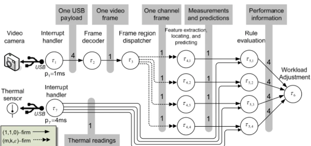
Fig. 6. A real-time surveillance system monitoring fishes in a fish tank. 1 τ τ2 τ3 τ4,1 2 , 4 τ 4 , 4 τ 3 , 4 τ 1 , 5 τ 2 , 5 τ 4 , 5 τ 3 , 5 τ 6 τ 7 τ firm (1,1,0)− firm ) k, (m,ε− 1ms p1= 4ms p₇= 4 4 4 4 4 1 1 1 1 1 1 1 1 1 1

Fig. 7. Interactions of tasks in the surveillance system for demonstration.

system to monitor fishes in a fish tank. The application was a part of a biological re-search project, in whichdynamics of a group of fishes were analyzed based on real-time datacollection. The system was built over an embedded computingplatform, on which an ARM processor and 16 MB of RAM were adopted.The processor was normally rated at 200 MHZ. As shown in Fig.6, a video camera and a thermal sensor wereconnected to the system via USB. The resolution and frame-rate ofthe video stream delivered by the camera were 352 × 288 pixels and25 fps, respectively. We chose to modifyand port the OpenCV package [10] onto the targetplatform. The tracking ofvisual objects in video streams was based on the Lucas-Kanadeoptical-flow algorithm [11], and Kalman filters [12] were used to estimatethe trajectories of moving objects. An instance of the Kalman filterwas created for each visual object and the prediction provided by thefilter was used to refine the result of the optical-flow algorithmso as to reduce trajectory losses.

There were twenty guppies in the fish tank. Normally the processor has been al-ready overloaded if all twenty fishes need to be tracked. Thus weproposed to split the video stream into four channels bypartitioning every frame into four equal-sized regions, as shown inthe right-hand side of Fig. 6. The intention isto flexibly allocate processor time among the channels so as to paymore attention to those active objects and, at the same time, toslow down the monitoring of inactive objects. As shown in Fig. 7, the

de-livery of channel frames from task τ3 to instancesof task τ4 was subject to different (m, k, ε)-firm constraints for workload scaling. To conduct experiments, a pre-recorded 20-minute video was projected onto a small white screen and the vision was then cap-tured by theUSB camera.

Two performance metrics were adopted. The first is the average of the Root-Mean- Square errors between actual positions and predicted positions of visual objects. The lower the errors, the more accurate the tracking is. The other metric is responsiveness, which is the time between the ground-truth time of an occurrence of a particular scenario and the time the scenario is detected by the system. The shorter the time, the higher the responsiveness is.

Let the proposed firm-real-time-based event-driven approach be referred to as FE approach. An alternative approach was developed for performance comparison: Let all tasks in the system beindependent and periodic. For workload adjustment, the periods of channel-frame delivery from task τ3 to instances of taskτ4 were proportionally scaled. Let the approach be referred toas PP approach. More details on PP approach would be includedin the later sections.

5.2 Visual-Object Tracking Accuracy

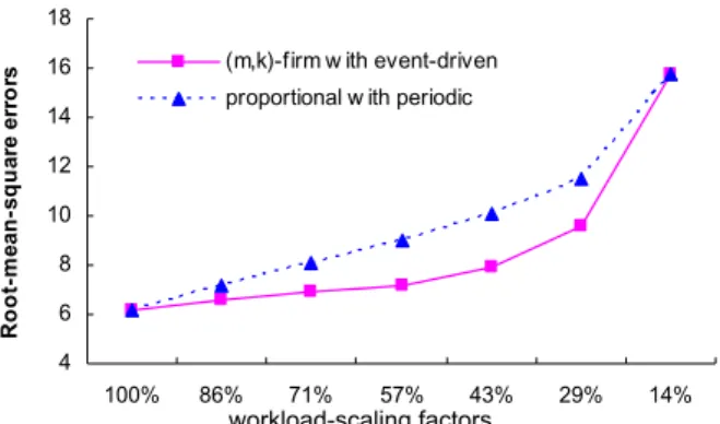
Let first only one of the four channels is enabled, and all the other three channels are ignored by the processor. In other words, the flow of τ1 → τ2 → τ3 → τ4,1 → τ5,1 → τ6 is enabled. Processor time available to the system was controlled by a parameter work-load-scaling factor for both FE approach and PP approach. A workload-scaling factor reflected a percentage of availableprocessor utilization. For FE approach, with respect to workload-scaling factor x/y, the delivery of channel frames fromtask τ3 to task τ4,1 was subject to (x, y, 0)-firm constraint. On the other hand, for PP approach, periods of task τ4,1 and task τ5,1 were proportionally enlarged bymultiplying their periods by y/x. In the experiments, sevenworkload-scaling factors were considered: 7/7 = 100%, 6/7 = 86%, 5/7 = 71%, 4/7 = 57%, 3/7 = 43%, 2/7 = 29%, and 1/7 = 14%. Forexample, with respect to workload-scaling factor 57%, under FEapproach, frame delivery from task τ3 to task τ4,1 wouldbe subject to (4, 7, 0)-firm constraint. Under PP approach, theperiods of task τ4,1 and task τ5,1 would both beenlarged from 4 ms to 4 × 7/4 = 7ms. Because 7 is a prime number,under anyone of the seven work-scaling factors (except 7/7 and1/7), the inter-arrival times of jobs of task τ4,1 under PPapproach and under FE approach would not be the same (and so werethose of jobs of task τ5,1).

The experimental results for the only one enabled channel were shown in Fig.8, in which the X-axis denoted theworkload-scaling factors and the Y-axis denoted the aver-age RMS errors. The figure showed that, even when the workload-scaling factor was decreased to 57%, FE approach could still kept the average RMS errors as small as if there were no frames skipped (i.e., 100%). The average RMS error significantly grew under a very small workload-scaling factor because the tracking of visualobjects was ineffective when a lot of frames were skipped. A similarphenomenon was observed for PP approach, however it imposed a relatively larger average RMS errors than the FE approach did whenthe workload-scaling factor was between 86% and 29%. The ration-ale would be explained later. Note that PP approach and FE approach resulted in the same average RMS errors when theworkload-scaling factor were 7/7 = 100% and 1/7 =

4 6 8 10 12 14 16 18 100% 86% 71% 57% 43% 29% 14% R oot-me an -s qua re e rr o

rs (m,k)-firm w ith event-driven

proportional w ith periodic

workload-scaling factors

Fig. 8. RMS errors resulted by different workload-scaling factors under the proposed event-driven paradigm and the purely periodic system.

i τ ' j τ " j τ _((0,2,4),FE _(4,7,0)) (0,2,7) PP (0,1,4)

Fig. 9. A scenario for workload scaling, where task τi = (0, 1, 4) and τj = (0, 2, 4) are a pump and the consumer (not shown), respectively. Let the workload-scaling factor be 4/7. Under PP approach and under FE approach we have τj′ = (0, 2, 7) and τj′′ = ((0, 2, 4), (4, 7, 0)), re-spectively.

14%. That was because, with respect to 7/7 or 1/7, the inter-arrival times of channel frames under the two approaches were the same.

One advantage of FE approach over PP approach is that the“absolute” inter-arrival time of any two successive events is exactlyknown. Consider the scenario shown in Fig. 9:Producer τi = (0, 1, 4) handles a periodic hardware event and sendevents to consumer τj = (0, 2, 4) with ri,j = 1. Now let theworkload-scaling factor for the delivery of events be 4/7 = 57%.Under PP approach consumer τj became τj′ = (0, 2, 7) andunder FE ap-proach it became τj′′ = ((0, 2, 4), (4, 7, 0)). As shownin Fig. 9, τj′ assumed that the in-ter-arrivaltime of events was pj = 7. However, it can be seen that theinter-arrival times of the first four events were actually 0pi, 1pi, 3pi, and 5pi. Conversely, under FE ap-proach, the inter-arrivaltimes of events could be calculated for τj′′ based on Eq.(2) and Corollary 1. To exactly know the inter-arrival times of events is very important to tim-ing-sensitive algorithms such as Kalman filters. With the absolute time of the current event, Kalman filters need to know when the prior event arrived and when the next event will arrive for refinement and prediction, respectively.

With multiple channels, this part of experiments was focused onevaluating whether or not processor time could be effectivelyallocated among channels for accurate tracking.

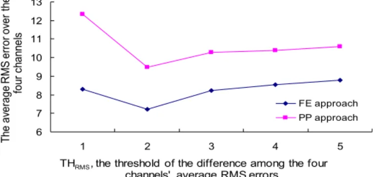
Now all four channels are enabled for experiments. A naive workload adjustment policy (i.e., task τ6) was adoptedfor both FE approach and PP approach. The following illustra-tion wasbased on FE approach: Let the delivery of channel frames from taskτ3 to tasks τ4,1, τ4,2, τ4,3, and τ4,4 be subject to (m, k, ε)-firm constraint chosen from{(1, 7, 0), (2, 7, 0), (3, 7, 0), (4, 7, 0), (5, 7, 0), (6, 7, 0),(7, 7, 0)}. Each time when task τ6 was invoked, it picked thechannel which was of the largest average RMS error. Ties were broken arbi-trarily. Suppose task τ4,i corresponded to the chosenchannel. Task τ6 tried to promote (mi,

ki, εi)(e.g., from (3, 7, 0) to (4, 7, 0)). Let THRMS be a predefinedsystem parameter for the threshold of the maximum difference betweenthe average RMS errors of any two channels. If the workload couldnot be admitted by the test in Theorem 2, some proce-dures were taken: Let τ4,j correspond the channel which had the smallest average RMS error. τ6 tried to demote (mj, kj, εj) (e.g., from(5, 7, 0) to (4, 7, 0)). The demotion was repeated until the resulted workload was schedulable. If all possible adjustments to workloadswere not admitted, all changes were reverted. Note that, based onproportional period adjustment; workload adjustment for PP approach was done similarly. But the difference is that PP adjusts task periods.

The experimental results were presented in Fig. 10, where the X-axis denoted dif-ferent settingsof the threshold THRMS and the Y-axis denoted the average RMSerror over the four channels. As we can see, FE approachsignificantly outperformed PP approach no matter what THRMSwas. Because PP approach was less effective in tracking objects than FE approach was (as shown in the previous section), for onesingle channel to re-duce it’s average RMS error PP approach could require more CPU utilization than FE approach did, and consequentlyprocessor utilization available to the monitoring of other channelsbecame small. We must point out that a very small setting ofTHRMS could result in frequent workload adjustments (i.e., when THRMS = 1), which usually incorrectly slowed down the monitoringof some channels which needed a lot of attentions.

6 7 8 9 10 11 12 13 1 2 3 4 5 FE approach PP approach errors RMS average channels'

,thethresholdofthedifferenceamongthefour THRMS ch an nel s fou r th e ov er erro r RM S av erage The

Fig. 10. The overall average RMS error resulted by the FE approach and the PP approach under different settings of the difference threshold of average RMS errors of channels (i.e.,

THRMS).

5.3 Responsiveness

This section provides evaluations of the two approaches’responsiveness. Respon-siveness was evaluated in terms of the timeinterval between the ground-truth time of a

scenario’s occurrenceand the time when the occurrence was detected. The time interval isreferred to as the response time hereafter. The ground-truthtime of the occurrences of a scenario was first measured from thevideo stream by off-line analysis, and during run- time the scenario was defined as a rule to be evaluated by task τ5. From the off-line analysis, the ground-truth number of scenario occurrenceswas 32.

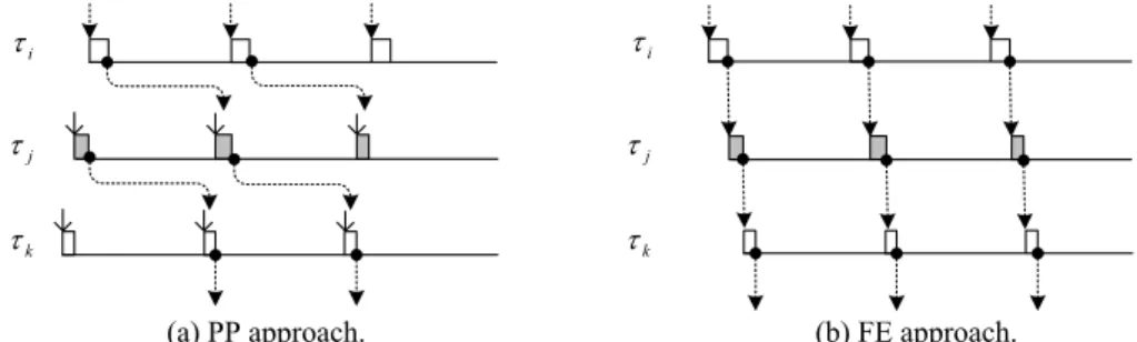
The experimental results were shown in Table 1.Compared to the results of PP ap-proach, FE approach showed significantly reduced average response time. The phe-nomenon was dueto misalignments of task jobs of PP approach: Consider the taskchain with ri,j = rj,k = 1 shown Figs. 11 (a)and (b). Because under PP approachany task job needed only to complete before its task period, a lengthy delay could be resulted as events were propagated among task jobs if they were not aligned. Such a phenomenon would be exaggerated when the periods of consumers and producers were relatively prime to each other because most task jobs were misaligned. The response time of the scenario shown in Fig.11 (a) could potentially go up topi + pj + pk. On the other hand, with respect to FE approach shownin Fig. 11 (b), a job of task τk mustcomplete before the upcoming job of task τi arrived, andconsequently the worst-case response time was bounded by pi. In addition, as showed in Table 1, four scenario occurrences were not detected by PP approach due to ineffective tracking. The number of undetected occur-rences was only two under FEapproach.

i τ k τ j τ i τ k τ j τ

(a) PP approach. (b) FE approach.

Fig. 11. Scenarios of FE approach and PP approach in responding hardware events, where ri,j = rj,k = 1.

Table 1. The average response time of PP approach and FE approach.

(The ground-truth number of scenario occurrences was 32 in the pre-recorded video)

The average response time (ms) The number of scenario occurrences detected

The FE approach 5.41 30

The PP approach 3.22 28

6. CONCLUSION

This paper considers a workload scaling mechanism foruniprocessor real-time em-bedded systems. The design objectives are to hide complex precedence constraints among tasks from outside, and to expose a set of simple but effective primitives for workloadscaling. A new approach that combines firm-real-time scheduling andan event- driven paradigm is proposed: The feeding of externalhardware events are controlled by a

deterministic algorithm, and dependencies among task jobs are formulated as events. Because taskjobs are triggered by events, the whole system automatically reactsto when and how external hardware events are fed in. We also showthat, with our approach, the system still have deterministic timingbehaviors, thus timing-sensitive algorithms such as Kalman filters arebenefited a lot. An on-line admission control policy is proposed sothat system timing correctness can be verified before any changes toworkloads can be made. A series of experiments were conducted on areal-time surveillance system based on the proposed approach.Experimental results showed that, under heavily stressing workloads, the proposed approach still provided better accuracy and higherresponsiveness for visual object tracking than a system using proportional period adjustment for purely periodic tasks.

REFERENCES

1. K. Jeffay, “The real-time producer/consumer paradigm: aparadigm for the construc-tion of efficient, predictable real-timesystems,” in Proceedings of ACM Symposium

on AppliedComputing, 1993, pp. 796-804.

2. A. K. Mok and W. Wang, “Window-constrained real-time periodic taskscheduling,” in Proceedings of the 22nd IEEE Real-Time Systems Symposium, 2001, pp. 15-24.

3. R. West and C. Poellabauer, “Analysis of a window-constrainedscheduler for real- time and best-effort packet streams,” in Proceedings of the 21st IEEE Real-Time Systems Symposium, 2000, pp. 239-248.

4. G. Koren and D. ShaSha, “Skip-over: algorithms and complexity foroverloaded sys-tems that allow skips,” in Proceedings of the 16th IEEE Real-Time Systems Sympo-sium, 1995, pp. 110-117.

5. P. Ramanthan, “Overload management in real-time control applications using (m,

k)-firm guarantee,” IEEE Transactions onParallel and Distributed Systems, Vol. 10,

1999, pp. 549-559.

6. M. Hamdaoui and P. Ramanathan, “A dynamic priority assignmenttechnique for streams with (m, k)-firm deadlines,” IEEE Transactions on Computers, Vol. 44,

1995, pp. 1443-1451.

7. C. L. Liu and J. W. Layland, “Scheduling algorithms formultiprogramming in a hard real-time environment,” Journal of the ACM, Vol. 20, 1973, pp. 46-61.

8. J. Hill, R. Szewczyk, A. Woo, S. Hollar, D. E. Culler, and K. S. J.Pister, “System architecture directions for networked sensors,” in Proceedings of the 9th ACM In-ternational Conference on Architectural Support for Programming Languages and OperatingSystems, 2000, pp. 93-104.

9. W. K. Shih and J. W. S. Liu, “On-line scheduling of imprecise computations to minimize error,” in Proceedings of the 13th IEEE Real-Time Systems Symposium,

1992, pp. 280-289.

10. “The open computer vision library,” http://sourceforge.net/projects /opencvlibrary/. 11. B. Lucas and T. Kanade, “An iterative image registration techniquewith an

applica-tion to stereo vision,” in Proceedings of the 7th Internaapplica-tional Joint Conference on Artificial Intelligence, 1981, pp. 121-130.

12. G. Welch and G. Bishop, “An introduction to the Kalman filter,”Technical Report No. TR 95-041, Dept.of Computer Science, University of North Carolina, 1995.

13. K. Tindell and J. Clark, “Holistic schedulability analysis fordistributed hard real- time systems,” Microprocessing and Microprogramming, Vol. 40, 1994, pp. 117-134.

14. P. Richard, F. Cottet, and M. Richard, “On-line scheduling ofreal-time distributed computers with complex communication constraints,” in Proceedings of the 7th

IEEE International Conference onEngineering of Complex Computer Systems, 2001,

pp. 26-34.

15. K. Ramamritham, “Allocation and scheduling of precedence-relatedperiodic tasks,”

IEEE Transactions on Parallel and DistributedSystems, Vol. 6, 1995, pp. 412-420.

16. T. Y. Yen and W. Wolf, “Performance estimation for real-timedistributed embedded systems,” IEEE Transactions on Parallel and Distributed Systems, Vol. 9, 1998, pp.

1125-1136.

17. Y. Shin and K. Choi, “Rate assignment for embedded reactivereal-time systems,” in

Proceedings of the 24th EUROMICRO Conference, Vol. 1, 1998, pp. 237-242.

18. T. W. Kuo and A. K. Mok, “Incremental reconfiguration and load adjustment in adaptive realtime systems,” IEEE Transactions on Computers, Vol. 46, 1997, pp.

1313-1324.

19. T. Gustafsson and J. Hansson, “Data freshness and overload handlingin embedded systems,” Technical Report, http://www.ida.liu.se/~thogu/gustafsson06admission. pdf, 2006.

20. K. D. Kang, S. H. Son, and J. A. Stankovic, “Managing deadline missratio and sen-sor data freshness in real-time databases,” IEEE Transactions on Knowledge and Data Engineering, Vol. 16, 2004, pp. 1200-1216.

21. L. P. Chang, “Event-driven scheduling for dynamic workload scaling in uniprocessor embedded systems,” in Proceedings of the 21st ACM Symposium on Applied

Com-puting, 2006, pp. 1462-1466.

Li-Pin Chang(張立平) received his Ph.D. and M.S. degrees

from Department of Computer Science and Information Engi-neering, National Taiwan University, Taipei, Taiwan, in 2003 and 1997, respectively. After two years of military service in Judicial Yuan, Taiwan, he serves as Assistant Professor at Department of Computer Science, National Chiao Tung University, Hsinchu, Taiwan, since 2005. His current research interests are of two main themes: real-time computing, and embedded storage systems.

Ya-Shu Chen (陳雅淑) received her B.S. degree from

Na-tional Chiao Tung University, Taiwan, R.O.C., in 2001. She re-ceived her M.S. and Ph.D degree from National Taiwan Univer-sity, Taiwan, R.O.C., in 2003 and 2007, respectively. She serves as Assistant Professor at Department of Electrical Engineering, National Taiwan University of Science and Technology, since 2007. Her current research interests include real-time systems, embedded systems, and system-on-a-chip.