Limit Cycle Analysis of Nonlinear
Multivariable Feedback Control Systems
bJ’ TAIN-SOU TSAY and KUANG-WE1 HANInstitute of Electronics, Department of Electrical Engineering, National Chiao-Tung University, Taiwan, Republic of China
ABSTRACT : A practical method is presented for the analysis of limit cycles in multivariable feedback control systems having separable nonlinear elements. The limit cycles are found by
use of a criterion generated by the stability-equation method. Numerical examples are given and compared to other methods in the current literature.
I. Introduction
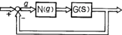
In this paper, a practical method is presented which can be used to analyse the limit cycles of nonlinear multivariable feedback control systems having separable nonlinear elements. The general configuration of the considered nonlinear systems is shown in Fig. 1, where N(a) and G(S) represent the nonlinear and linear parts of the system, respectively. The method is based upon the stability-equation method which has been widely used for single-input-single-output nonlinear feedback control systems (l-5). The basic approach is to consider the equivalent gains of the nonlinearities as parameters to be analysed in the parameter-plane (l-5), and then the describing-function method is used to evaluate the amplitudes of the limit cycles at the inputs of nonlinearities.
In current literature, for multivariable systems the Nyquist, inverse Nyquist, and numerical optimization methods are usually used to predict the existence of limit cycles. These methods are based upon the graphical or numerical solutions of the linearized harmonic balance equations (614). It has been shown that, for multivariable systems, over arbitrary ranges of amplitudes (AJ, frequency (CO) and phases (QJ, an infinite number of possible solutions may exist (14). Gray has proposed a sequential computational procedure to seek the solutions for only specified ranges of discrete values of Ai, o and Oj (12-14) ; these specified ranges are determined by use of the Nyquist or inverse Nyquist plots. Although the aforementioned methods are powerful, large computational efforts are usually required.
3
I’
IIFIG. 1. A general block diagram of nonlinear multivariable feedback control systems.
simple.
II. The Basic Approach
Consider the system shown in Fig. 1. The linearized harmonic balance equations (12-14) governing the existence of limit cycles can be expressed as :
[G(S)N(a) +I]a = 0, (1)
where N(a) is a matrix of describing functions of the nonlinear elements, and a is a column vector of sinusoidal inputs to these nonlinear elements, such that
aj = Ai exp [j(ot+eJ] (i= 1,2 ,..., n), (2)
where Ai are the amplitudes of a,; Qi are the phase angles about a reference input ; and II is the number of nonlinearities.
From (1) and (2), one can see that the number of parameters to be found is larger than that of the linearized harmonic balance equations. Therefore, an infinite number of possible solutions (14) exist which can satisfy (1).
For illustration, assume that a 2 x 2 nonlinear multivariable system with two single valued nonlinearities in the diagonal terms is considered ; the block diagram is shown in Fig. 2. The harmonic balance equations (614) of loop 1 and loop 2 are
Al ejelNl(a,)gl,(jo)+A, ej’ZN2(a,)g,2(jw) = -Al eiel (3)
Al eje~N,(al)g,,(jw) +A2 eis2N2(a2)g22(jm) = -AZ e@z (4)
respectively, where g,(S) are the (i, j) elements of G(S) ; Nl(al) and Nz(az) are the describing functions [or equivalent gains (15, 16)] of the nonlinearities N, and N2, respectively.
Consider the input of Ni as the reference input. Then one has 8, = 0, and (3) gives
:
(5)
Similarly, (4) gives
Analysis of Control Systems
(6)
Equating (5) and (6), one has
F(@) = l+N~(ak~~(j~)
+N&)gA@)
~~~~~~~~~~~~~~~~~~~~~~~~~~~~~~~~~~~~~~~~~~~~
= 0
(7)
which is the characteristic equation of the considered system. Note that N1 (a J and
N,(aJ
areconsidered as variable parameters.
Equation (7) can be decomposed into two stability equations (l-5)
;i.e.
F,(o) = B,(w)+N,(a,)C,(co)+N,(az)ol(o)+Nl(a,)Nz(a,)El(o)
= O (8)
and
F,(o) = B2(0)+N1(a,)Cz(o)+Nz(a2)oz(~)+N*(a,)N*(a2)Ez(o)
= O. (9)
Equation (8) gives
N&d = -
Bl(~)+Nl(aACl(~)
~l(~)+Nl@dEl(o)’
Similarly, (9) gives
N2(a2) = -
~2(~)+N~(aX’d~)
D2(u)+Nl(aM2(o)
(10)
(11)
Equating (10) and (1 I), one has
[C,(~~)E,(~)-C,(~)E,(~)~N,(~,)‘+ICZ(CO)D~(~)+BZ(~)EI(~)
-c,(o)D,(o)--B,(w)E,(w)lN,(a,)+[B2(co)Dl(w)--B,(w)D2(w)l
= 0. (12)
For specified values of frequency (w), the values of Nl(al) can be found by
solving (12)
;the corresponding values of N,(a,) can be found from (lo), (11). For
a number of suitable values of CD,
the real solutions of N,(aJ and N,(a2) can be
plotted in a Nl(aJ vs N2(a2) plane. The typical result for a latter example is shown
in Fig. 3.
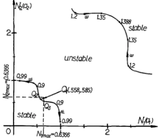
FIG. 3. Root-loci of the stability-equations for Example 1 with K = 2.
Vol. 325, No. 6, pp. 721-730, 1988
(i) Every point on the curves, as shown in Fig. 3, represents a set of N,(a,), N2(aJ and CO, which can satisfy the condition of having a limit cycle ; i.e. the roots oei and wOi of the even and odd stability equations F,(o) and FJo(w), respectively, are all real and alternative in sequence except that one root pair is equal to each other (i.e. oei = wOi = CO) (Z-S). But for nonlinear multivariable systems, an infinite number of solutions can satisfy this condition (14). This is quite different from the single-input-single-output system.
(ii) If the root-loci as shown in Fig. 3 separate the stable and unstable regions, then a limit cycle may exist. The reason is that the system will become stable or unstable when the amplitudes Aj increase or decrease. In other words, if the system becomes stable (unstable) when the amplitudes Aj increase (decrease), a stable limit cycle may exist at the stability boundary (2-5).
(iii) A limit cycle may exist only if the values of Nl(al) and N,(a,) are less than the maximal gains (N,,,, and N Zmax) of the nonlinearities N1 and N2 ; e.g. in Fig. 3, the useful solution may exist only in the section between points Qz and Q3. (iv) A limit cycle may exist if the roots NI(al) and N,(a,) satisfy (3) and (4). From (3) and (4), the possible solution can be found by equating the real and imaginary parts of (5) and (6), respectively ; i.e.
jejo,, _e@z6] = 0 (13)
where eZ5 and QZ6 represent the phase angles found by (5) and (6), respectively. Therefore, the values of A 1, A 2 and CO, for having a limit cycle, can be found from (g), (9) and (13).
If the considered nonlinear system satisfies all of the above four conditions, a limit cycle will exist. More explanations are given along with the numerical ex- amples given in the next section.
IZZ. Examples Example 1
Assume that the system shown in Fig. 2 is a 2 x 2 system with transfer function matrix (11)
G(S) = K 2[ -o.2;-o.2 :.;I
s(s+ 1) (14)
where Krepresents the loop gains. The nonlinearities are two identical on-off relays with dead-zones having unit switching level and unit height.
From (7), the characteristic equation of the closed-loop system is F(S) = S6+4S5+6S4+4S3+S2+KNl(al)(S3+2S2+S)
+KNz(a2)(S3+2S2+S)+K2N1(a1)N2(a2)(0.06S+1.06) = 0. (15)
Analysis of Control Systems
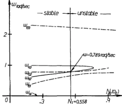
FIG. 4. Root-loci of wei and woi of the stability-equations with fixed Nl(a,) and varying N&Z>. F,(o) = -~6+6~4-u?+KN1(a1)(-2~2)+KN~(a,)(-2d) +K2NI(aI)N2(a,)(1.06) = 0 (16) and F,(o) = 405-4c03+KN1(a1)(-~3++)+KN2(aa)(-c03+o) +K2Nl(al)N2(a2)(0.06co) = 0. (17)
For K = 2, and for a number of frequencies o, the simultaneous solutions [N,(a 1)
and Nz(a2)] of (16) and (17) are calculated and represented by two root-loci, as shown in Fig. 3, where the stability of each region is also shown. At every point on the root-loci, the roots oei and ooi of the stability-equations Fe(o) and F,(o) are all real and alternative in sequence except that one root pair is equal to each other (i.e. wei = ooj = w).
In Fig. 3, it can be seen that the section between points Q2 and Q3 can satisfy conditions (i) to (iii). Solving (13) in this section, one has a limit cycle at point Qi (0.558, 0.585) with oscillating frequency o = 0.789 rad s-l, and amplitudes
AI = 1.964 and AZ = 1.818. This fact is supported by checking the roots wCj and
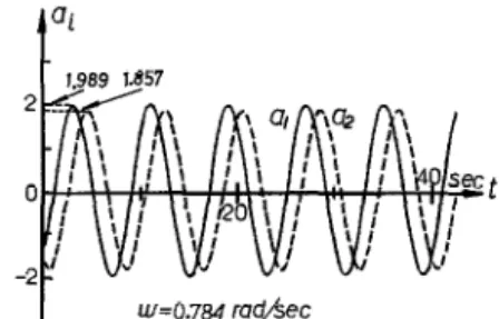
ooj of the stability-equations in the neighborhood of Qr (5). Figure 4 shows that the loci of oei and woj for N,(a,) is fixed at 0.558 and N,(a,) is varying. From Fig. 3, one can see that if the value of N,(aJ is less (larger) than 0.585, the roots oei and woj are (not) alternative in sequence and the corresponding system is stable (unstable) (2-5). Therefore, a stable limit cycle will exist at the stability-boundary where N2(a2) = 0.585. Similar results can be obtained when N,(a,) is lixed at 0.585 and N,(al) is varying. By computer simulation, Fig. 5 shows the limit cycle of the system for K = 2.
In current literature, the purpose of analysis is to find the minimum value of K for just having a limit cycle. In this paper, for various values of K the locus of Qr can be plotted easily, as shown in Fig. 6, where the minimum value of K is at point Qlm, where the values of N,(a,) and N,(aJ are just equal to the maximum values
Vol. 325, No. 6, pp. 721-730, 1988
FIG. 5. The simulated limit-cycle of Example 1 for K = 2.
8
M(4)
Q‘b
qm(o.6366, 0.6366) $ ___ __-___ 2- ,I:‘,” 0.5 iA
4. I 6 I I 1 , lOI) 0 0.5 rJ,m=o.sja; 1 FIG. 6. Locus of Q , vs K. TABLE IThe gains K for just having a limit cycle in Example I Methods Gain K Proposed method 1.79 Aizerrnan Conjecture 1.79 Hirsch plot 1.25 Mee plot 1.50 Digital simulation 1.787
of the describing functions. For the system considered, the minimum value of K is found at 1.7924. From Ref. (ll), the results obtained by the use of other methods, are shown in Table I. Although all the results are approximately the same, the proposed method is relatively simple in computation.
Example 2
Consider a nonlinear system with transfer function matrix (16)
K 16S2+23S+9 4s2-s-3
G(S) = m W-s-3 16S2+23S+9
1
(18)
Analysis of Control Systems
___,
/R_
___I$;
(QJ Ib)
FIG. 7. Nonlinearities of Example 2.
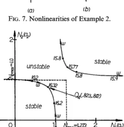
FIG. 8. Root-loci of stability equations for Example 2 with K = 2.
-2 t
W=I~.~IKIC&, A,=/46z,A2=/45/
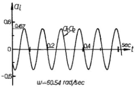
FIG. 9. The simulated limit-cycle of Example 2 for K = 2.
and N2 are different, as shown in Fig. 7. Similar to the procedure stated in Examjple 1, the root-loci of the stability-equations for K = 2 are plotted, as shown in Fig. 8, where point Q4 (0.823, 0.812) with oscillating frequency o = 16.32 rad s-l, and amplitudes Al = 1.454 and A2 = 1.427 can satisfy all the conditions of having a limit cycle. Figure 9 shows the simulated limit cycle of the system, in which a, is almost identical to a2. It can be seen that the simulated results are quite close to those obtained by calculation.
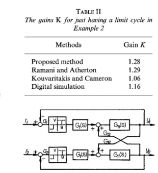
Table II shows the values of K for just having a limit cycle predicted by various methods (8, 16).
Example 3
Consider a coupled-core reactor (17,lS) with system configuration, as shown in Fig. 10, where
Vol. 325, No. 6, pp. 721-730, 1988
and
Example 2
Methods Gain K
Proposed method 1.28
Ramani and Atherton 1.29 Kouvaritakis and Cameron 1.06 Digital simulation 1.16
b + a v--
---@=Q B CT&) + + G&) 1
I I
FIG. 10. Block diagram of a control system for a coupled-core reactor.
G,,(S) =
(S+a)(S+4 (S+A)(S+a)+ tS(S+a)+ ?(S+d) (19) G,2(S) = ; G,(S) =no
zS(l+ T,S)’(20)
(21)
Assume that the parameters of the system are p = 0.0049,1 = 0.44, z = 0.0001 s, h = 10”F/(MW s), a = 10 s-l, M = O.OOl”F-‘, yto = 30 MW, r = 0.018, T, = 0.07 s, and the parameters of the nonlinearities, shown in Fig. 10, are B = 0.25 MW and V = M x 10e3 skjk - s (17, 18). For M = 22, by use of the same procedure stated in Example 1, the root-loci of the stability-equations are shown in Fig. 11, where point Qs (0.052, 0.052) with oscillating frequency o = 60.93 rad s- ‘, and amplitudes A, = 0.446 MW and A2 = 0.446 MW satisfies all the conditions of having a limit cycle. The simulated result is shown in Fig. 12. (Note that a, is identical to a2 because the considered system is symmetrical.) This is quite close to that obtained by calculation.From all the above examples, it can be seen that the proposed method provides a simple way for predicting the existence of limit cycles of nonlinear multivariable feedback control systems, and that in each system a unique solution can be obtained using simple calculations.
Analysis of Control Systems
FIG. 11. Root-loci of stability equations for Example 3.
FIG. 12. The simulated limit-cycle of Example 3 for M = 22 and B = 0.25 MW.
IV. Conclusions
In this paper, a method for limit cycle analysis in nonlinear multivariable feed- back control systems has been presented, and found to be simpler than other methods given in the current literature. It has been shown that the proposed method can be easily applied to very complicated systems.
References
(1) K. W. Kan and G. J. Thaler, “High Order System Analysis and Design using the Root Locus Method”, J. Franklin Inst., Vol. 281, No. 2, pp. 99-113, Feb. 1966.
(2) K. W. Han, “Nonlinear Control System : Some Practical Method”, Academic Culture Company, 1977.
(3) Y. L. Chen and K. W. Han, “Stability Analysis of a Nonlinear Reactor Control System”, IEEE Trans. Nucl. Sci., Vol. NS-17, No. 2, pp. 18-25, April 1970. (4) C. H. Ai and K. W. Han, “Stability Analysis of Nuclear Reactor Control System with
Multiple Transport-lags and Asymmetrical Nonlinearity”, IEEE Trans. Nucl. Sci.,
Vol. NS-22, No. 5, Oct. 1975.
(5) T. S. Tsay and K. W. Han, “Analysis of a Nonlinear Sampled-data Proportional Navigation System having Adjustable parameters”, J. Franklin Inst., Vol. 321, No. 4, pp. 203-218, April 1986.
(6) D. P. Atherton, “Nonlinear Control Engineering”, Van Nostrand-Reinhold, London, 1975.
Vol. 325, No. 6, pp. 721-730, 1988
(8) (9) (10) (11) (12) (13) (14) (15) (16) (17) (181
N. Ramani and D. P. Atherton, “Frequency Response Method for Nonlinear Multivariable Systems”, Canadian Conference on Automatic Control, University of New Brunswick, Fredericton, 1973.
N. Ramani and D. P. Atherton, “A Describing Function Method for the Approximate Stability of Nonlinear Multivariable Systems”, University of New Brunswick, Elec- trical Engineering Department, Report SDC- 1, 1975.
S. Shankar and D. P. Atherton, “Graphical Stability Analysis of Non-linear Multivariable Control Systems”, Znt. J. Control, Vol. 25, pp. 375-388, 1977. A. K. El Shakkany and D. P. Atherton, “Computer graphics method for Nonlinear
Multivariable Systems”, IFAC Computer-Aided Design of Control Systems, pp. 157-161, 1979.
J. 0. Gray and P. M. Taylor, “Frequency Responses Method in the Design of Multivariable Nonlinear Feedback Systems”, 4th IFAC, Multivariable Tech- nological Systems, pp. 225-232, 1977.
J. 0. Gray and P. M. Taylor, “Computer Aided Design of Multivariable Nonlinear Control Systems using Frequency Domain Techniques”, Automatica, Vol. 15, pp. 281-297, 1979.
J. 0. Gray and N. B. Nakhla, “Prediction of Limit Cycle in Multivariable Nonlinear Systems”, PROC. IEE, Vol. 128, Pt.D, pp. 283-241, Sept. 1981.
R. G. Cameron and M. Tabatabai, “Prediction of the Existence of Limit Cycles using Walsh Function: some Further Results”, ht. J. System Sci., Vol. 14, pp. 1043-
1064, 1983.
B. Kouvaritakis and R. G. Cameron, “The Use of Walsh Functions in Multivariable Limit Cycle Prediction”, Automatica, Vol. 19, pp. 5133522, 1983.
G. V. S. Raju and R. S. Stone, “Control System in Spatially Large Cores”, IEEE Trans. Nucl. Sci., Vol. NS-17, pp. 534540, Feb. 1970.
N. Tsouri, J. Rootenberg and L. J. Lidofsky, “Stability Analysis of a Reactor Control System by the Tsypkin Locus Method”, IEEE Trans. Nucl. Sci., Vol. NS-20, No. 1, pp. 649-660, Feb. 1973.