Video Algebra for Spatio-Temporal Reasoning
of Iconic Videos Represented in 3D C-string
ANTHONY J. T. LEE, PING YU, HAN-PANG CHIU*AND HSIU-HUI LINDepartment of Information Management National Taiwan University
Taipei, 106 Taiwan
*Department of Electrical Engineering and Computer Science
Massachusetts Institute of Technology Cambridge, MA 02139, U.S.A.
The video content management has attracted increasing attention in recent years. We have proposed a new spatio-temporal knowledge structure, called 3D C-string, to represent the spatio-temporal relations between the objects in a video and to keep track of the motions and size changes of the objects. In this paper, we propose a video algebra to infer the spatio-temporal relations between the objects in a video represented by the 3D C-string. The algebra contains four kinds of rules, namely, transitive, distributive, manipulation, and integration rules. By using those rules, all the binary relations between the objects in a video can be derived from a given 3D C-string. The algebra provides the theoretic basis for spatio-temporal reasoning and video query inference.
Keywords: video algebra, spatio-temporal relation, 3D C-string, video database, spatio-
temporal reasoning
1. INTRODUCTION
With the advances in information technology, the amount of multimedia data cap-tured, produced and stored is increasing rapidly, and hence, the need for organizing this data and accessing it from a vast amount of repositories has attracted much attention in recent years. Over the last decade, many image/video indexing and retrieval methods have been proposed. Bimbo et al. [1] developed a prototype system of image sequence retrieval, where video frames were processed and simple events were represented by spa-tial-temporal logic (STL). Chang et al. [2] proposed a model called VideoQ to analyze objects’ motions in a video and provide an efficient and effective content-based retrieval mechanism. Naphade et al. [3] proposed a model to map low-level features to high-level semantics and to enforce spatio-temporal constraints in a factor graph framework. Ngo et
al. [4] proposed a motion computation method based on a structure tensor formulation to
encode visual patterns of spatio-temporal slices in a tensor histogram and to describe the motion trajectories of moving objects. VideoQA [5] allowed users to use short natural language questions with implicit constraints on contents to retrieve short precise news video summaries. Lo et al. [6] presented a framework for retrieving video sequences us-ing successive modular operations on temporal similarity. Snoek et al. [7] developed the TIME framework to classify the semantic events in multimodal video documents.
Received November 18, 2004; revised August 18, 2005; accepted November 7, 2005. Communicated by Ming-Syan Chen.
In image database management systems, one of the most important methods for re-trieving the images is using the perception of objects and the spatial relations between the objects in the desired videos. To represent the spatial relations between the objects in an image, Chang et al. [8] proposed the concept of the 2D string in which the objects are projected onto the x- and y-axes to form two strings representing the relative positions of the projections in the x- and y-axes, respectively. This approach provides a natural way to construct iconic indexes for images and supports spatial reasoning and image queries. There are many follow-up approaches based on the concept of the 2D string including
2D G-string [9, 10], 2D C-string [11-13], 2D C+-string [14], 2D RS-string [15], 2D
C-Tree [16], unique-ID-based matrix [17], GPN matrix [18], virtual image [19], BP ma-trix [20], and 2D Z-string [21].
To represent the spatial and temporal relations between the objects in a symbolic video, many iconic indexing approaches, extended from the notion of the 2D string to represent the spatial and temporal relations between the objects in a video, have been proposed, for example, 2D B-string [22, 23], 2D C-Tree [24], 9DLT strings [25], 3D-list [26], and 3D C-string [27].
In the 3D C-string [27], we extended the concepts of the 2D C+-string and proposed
3D C-string to represent the spatio-temporal relations between the objects and to record their motions and size changes. We also developed the string generation and video re-construction algorithms for the 3D C-string. The string generated by the string generation algorithm is unique for a given video and the video reconstructed from a given 3D C-string is unique too. In comparison with the previously proposed approaches [22-26], there is one-to-one correspondence between strings and videos in the 3D C-string repre-sentation. This approach can provide us an easy and efficient way to retrieve, visualize and manipulate video objects in video database systems.
In this paper, we propose a video algebra for reasoning the spatio-temporal relations between the objects in a video represented by the 3D C-string. The algebra contains four kinds of rules, namely, transitive, distributive, manipulation, and integration rules. By using those rules, all the binary relations between the objects in a video can be derived from a given 3D C-string. The algebra can provide the theoretic basis for spatio-temporal reasoning and video query inference.
The rest of this paper is organized as follows. In section 2, a brief introduction of the 3D C-string approach is presented. The video algebra of reasoning the spatio-tem- poral relations between the objects in a video represented by the 3D C-string is discussed in section 3. In section 4, an application is presented to show the effectiveness of our proposed approach. Finally, concluding remarks are made in section 5.
2. 3D C-STRING APPROACH
In the knowledge structure of 3D C-string, we use the projections of objects to rep-resent the spatial and temporal relations between the objects in a video. The objects in a video are projected onto the x-, y-, and time-axes to form three strings representing the relations and relative positions of the projections in the x-, y- and time-axes, respectively. These three strings are called u-, v- and t-strings. The projections of an object onto the x-,
the 2D C-string and 2D C+-string, the 3D C-string has one more dimension: time
dimen-sion. So the 3D C-string is different from the 2D C-string and 2D C+-string that has only
spatial relations between objects, it has spatial and temporal relations. Hence, it is re-quired to keep track of the information about the motions and size changes of the objects in a video in the 3D C-string.
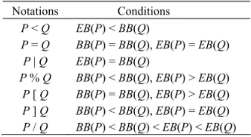
In the knowledge structure of 3D C-string, there are 13 relations for two one- dimensional intervals. For the x (or y) dimension, there are 13 spatial relations and its corresponding spatial operators have been presented in 2D C-string [11] as listed in Ta-ble 1, where BB(P) and EB(P) are the begin-bound (beginning point) and end-bound (ending point) of the x- (or y-) projection of object P. For example, in the x and y dimen-sions, P < Q represents that the projection of object P is before that of object Q. In the
time dimension, we also use those 7 operators to describe 13 possible relations between
two time-projections. According to [11], we know that all the 13 operators except “/” can precisely (no ambiguity) represent the relations between two objects. To avoid using op-erator “/”, we replace P/Q with P]Q|Q in the 3D C-string representation where Q is
called a cut object in P]Q|Q.
Table 1. The definitions of spatial operators in 2D C-string. Notations Conditions P < Q EB(P) < BB(Q) P = Q BB(P) = BB(Q), EB(P) = EB(Q) P | Q EB(P) = BB(Q) P % Q BB(P) < BB(Q), EB(P) > EB(Q) P [ Q BB(P) = BB(Q), EB(P) > EB(Q) P ] Q BB(P) < BB(Q), EB(P) = EB(Q) P / Q BB(P) < BB(Q) < EB(P) < EB(Q)
In the knowledge structure of 3D C-string, an object is approximated by a minimum bounding rectangle (MBR) whose sides are parallel to the x-axis and y-axis. For each object, we keep track of its initial location and size. That is, we keep track of the location and size of an object in its starting frame. After keeping track of the initial location and size of an object, we record the information about its motions and size changes in the 3D C-string.
There is some metric information defined in the 3D C-string, which is listed as fol-lows.
1. The size of object P: Ps denotes the size of the x- (y-, or time-) projection of object P, where s = EBx(P) − BBx(P) (s = EBy(A) − BBy(A), or s= EBtime(P) − BBtime(P)), where
BBx(P) and EBx(P) are the x coordinates of the begin-bound and end-bound of P’s
x-projection, respectively.
2. The distance associated with operator “<”: P <d Q denotes that the distance between the x- (y-, or time-) projection of object P and that of object Q is equal to d, where d =
BBx(Q) − EBx(P) (d = BBy(Q) − EBy(P), or d = BBtime(Q) − EBtime(P)).
the x- (y-, or time-) projection of object P and that of objectQ is equal to d, where d = BBx(Q) − BBx(P) (d = BBy(Q) − BBy(P), or d = BBtime(Q) − BBtime(P)).
4. The velocity and rate of size change associated with motion operators ↑v,r and ↓v,r: Operator ↑v,r denotes that the object moves along the positive direction of the x- (or y-) axis. Operator ↓v,r denotes that the object moves along the negative direction of the x- (or y-) axis. v is the velocity of the motion and r is the rate of size change of an object.
To represent the time intervals when the states of an object are changed, we intro-duce one more temporal operator |tin the 3D C-string. For example, P3 |t P5 denotes that
in the first 3 frames, object P remains in the same state of the motion and size change. However, from frame 4 to frame 8, the state of the motion and size changeof object P is changed into another. Note that in the 3D C-string representation, the motion operators are used to describe the states of motions and size changes, and the t-string is used to describe how long every state lasts.
In the 3D C-string representation, Lee et al. [27] also introduced the concept of tem-plate objects. A temtem-plate object is a pair of separators, “(” and “)”, containing a set of objects. For example, 0(A3 <2 B3) is a template object whose initial location is 0 and
whose size is 3 + 2 + 3 = 8.
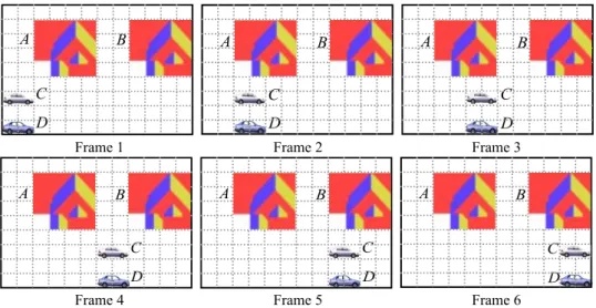
To see how 3D C-string works, let’s consider the following example as shown in Fig. 1. In this example, the video contains two still objects (houses) and two moving ob-jects (cars). All the obob-jects are approximated by the MBRs. Let’s consider how to gener-ate the u-string for the video. First of all, we project the initial locations of all objects onto the x-axis. Next, we scan the beginning and ending points of the objects from left to right to generate the u-string. We find that the x-projects of objects C and D are identical and both objects moves along the positive direction of the x-axis with the velocity of 2 pixels/frame, so we have (C2↑2,1 = D2↑2,1). The template object (C2↑2,1 = D2↑2,1) is joined
with the x-projection of object A, so we have ((C2↑2,1 = D2↑2,1)|A4). The difference
D A B C D A B C D A B C
Frame 1 Frame 2 Frame 3
D A B C D A B C D A B C Frame 4 Frame 5 Frame 6
(a) A video contains 6 frames. Fig. 1. An example video.
u-string: (((C2↑2,1 =D2↑2,1)|A4) <2 B4)
v-string: (D1↑0,1 <1 (C1↑0,1 <1 (A4 = B4)))
t-string: (A6 = B6 = C6 = D6) (b) The corresponding 3D C-string. Fig. 1. (Cont’d) An example video.
between the ending bound of template object ((C2↑2,1 = D2↑2,1)|A4) and the beginning
bound of the x-projection of object B is equal to 2, so we have (((C2↑2,1 = D2↑2,1)|A4) <2
B4). Note that since both objects A and B are still in the video, there is no velocity
associ-ated with them. The corresponding 3D C-string of the video is shown in Fig. 1 (b). Ob-jects C and D move along the positive direction of the x-axis with the velocity of 2 units/ frame in frames 1-6. Objects A and B do not move or change their sizes, so there are no motion operators for both objects. The knowledge structure of 3D C-string provides an easy and compact way to represent the spatial and temporal relations between the objects in a video.
3. INFERENCE RULES
In this section, we present the inference rules to derive the spatial and temporal rela-tions between each pair of objects in the 3D C-string. There are four kinds of fundamen-tal rules: transitive rules, distributive rules, manipulation rules and integration rules. In these inference rules, we abbreviate the velocities and rates of size changes since both of them are not changed in the inference process. After deriving the relation between two objects, we can obtain their velocities and rates of size changes from the given 3D C-string, and which can be easily applied to reasoning about spatio-temporal relations between the objects in a video.
Let R = {“<”, “|”, “=”, “[“, “]”, “%”, “|t”} be the set of relation operators. In the
time dimension, operator “|t” can be inferred as the same as operator “|”. First of all, let’s consider the 3-object strings of o1, o2, and o3, where oi, 1 ≤ i ≤ 3, may be a cut subobject (subobject for short), an object without any cutting (non-cut object for short) or a tem-plate object. There are three types of 3-object strings in the 3D C-string representation as follows, where L0 is the initial location associated with the template object represented by the 3-object string.
Type-I: L0(o1r12(o2r23o3)), where r12 and r23 ∈ R; however, r12 and r23 are not “=” at the
same time.
Type-II: L0((o1r12o2)r23o3), where r12 and r23 ∈ R; however, r12 and r23 are not “=” at the
same time.
Type-III: L0(o1r12o2r23o3), where both r12 and r23 are “=”. 3.1 Transitive Rules for a 3-Object String
For each type of strings, we can easily infer three binary relations between o1, o2,
λ2:L2(o r o2 23 3′ ), and λ3: L3(o r o1 13 3′ ). Each substring represents a template object which is associated with the initial location, namely L1, L2 and L3. If the initial location of the template object is equal to 0, it can be omitted.
Among them, it is easiest for a type-III string to derive the three binary relations by intuition, namely, L0(o1 = o2), L0(o2 = o3) and L0(o1 = o3). That is, the derived relation and metric information are the same as the original string. For a string of the first two types, the derived relations and metric information are shown in the following sections.
3.1.1 The relation transitive rules for type-I and type-II strings
The inferred binary relations of a 3-object string of type-I are shown in Figs. 2 (a-c). The inferred binary relations of a 3-object string of type-II are shown in Figs. 3 (a-c), where “N” denotes that the case is not available in the 3D C-string representation; “]*”, “*[“ and “%*” are the reverse relations of “]”, “[“ and “%”, respectively. That is, A]*B is equal to B]A. r23 r23 r23 12 r′ < ⏐ = [ ] % r′23 < ⏐ = [ ] % r′13 < ⏐ = [ ] % < < < < < < < < < ⏐ = [ ] % < < < < < < < ⏐ ⏐ ⏐ ⏐ ⏐ ⏐ ⏐ ⏐ < ⏐ = [ ] % ⏐ < < ⏐ ⏐ < < r12 = [ [ = [ ] = r12 = < ⏐ = [ ] % r12 = ] ] = [ ] % [ [ [ [ [ [ [ [ < ⏐ = [ ] % [ % % [ [ % % ] % % ] ] ] ] ] < ⏐ = [ ] % ] ] ] ] % ] % % % % % % % % % < ⏐ = [ ] % % % % % % % % (a) The inferred relation 12r′ (b) The inferred relation. 23r′ (c) The inferred relation. 13r′ .
Fig. 2. The inference relation tables for a type-I string.
r23 r23 r23 12 r′ < ⏐ = [ ] % r′23 < ⏐ = [ ] % r′13 < ⏐ = [ ] % < < < < N N N < < ⏐ [* N N N < < < [* N N N ⏐ ⏐ ⏐ ⏐ N N N ⏐ < ⏐ [* N N N ⏐ < < [* N N N r12 = = = = = = = r12 = < ⏐ = [ ] % r12 = < ⏐ = [ ] % [ [ [ [ N N N [ < < *[ N N N [ < ⏐ = N N N ] ] ] ] N N N ] < ⏐ ]* N N N ] < ⏐ = N N N % % % % N N N % < < %* N N N % < ⏐ = N N N (a) The inferred relation 12r′ (b) The inferred relation. 23r′ (c) The inferred relation. 13r′ .
Fig. 3. The inference relation tables for a type-II string.
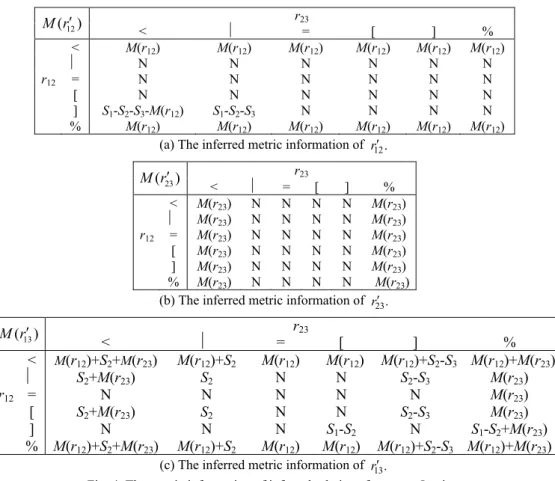
3.1.2 The metric information of the inferred relations for type-I and type-II strings The metric information of the inferred relations for a type-I string is listed in Fig. 4, where “N” denotes that there is not metric information for those cases, M(r) denotes the metric information of operator r and Si denotes the size of object i. The metric
r23 12 ( ) M r′ < ⏐ = [ ] % < M(r12) M(r12) M(r12) M(r12) M(r12) M(r12) ⏐ N N N N N N r12 = N N N N N N [ N N N N N N ] S1-S2-S3-M(r12) S1-S2-S3 N N N N % M(r12) M(r12) M(r12) M(r12) M(r12) M(r12)
(a) The inferred metric information of 12r′ . r23 23 ( ) M r′ < ⏐ = [ ] % < M(r23) N N N N M(r23) ⏐ M(r23) N N N N M(r23) r12 = M(r23) N N N N M(r23) [ M(r23) N N N N M(r23) ] M(r23) N N N N M(r23) % M(r23) N N N N M(r23)
(b) The inferred metric information of 23r′ . r23 13 ( ) M r′ < ⏐ = [ ] % < M(r12)+S2+M(r23) M(r12)+S2 M(r12) M(r12) M(r12)+S2-S3 M(r12)+M(r23) ⏐ S2+M(r23) S2 N N S2-S3 M(r23) r12 = N N N N N M(r23) [ S2+M(r23) S2 N N S2-S3 M(r23) ] N N N S1-S2 N S1-S2+M(r23) % M(r12)+S2+M(r23) M(r12)+S2 M(r12) M(r12) M(r12)+S2-S3 M(r12)+M(r23) (c) The inferred metric information of 13r′ .
Fig. 4. The metric information of inferred relations for a type-I string.
r23 12 ( ) M r′ < ⏐ = [ ] % < M(r12) M(r12) M(r12) N N N ⏐ N N N N N N r12 = N N N N N N [ N N N N N N ] N N N N N N % M(r12) M(r12) M(r12) N N N (a) The inferred metric information of 12r′ .
r23 23 ( ) M r′ < ⏐ = [ ] % < M(r23) N N N N N ⏐ M(r23) N N N N N r12 = M(r23) N N N N M(r23) [ S1-S2-M(r23) S1-S2 N N N N ] M(r23) N N N N N % S1-S2-M(r12)+M(r23) S1-S2-M(r12) M(r12) N N N (b) The inferred metric information of r′23.
r23 13 ( ) M r′ < ⏐ = [ ] % < S2+M(r12)+M(r23) S2+M(r12) N N N N ⏐ S2+M(r23) S2 N N N N r12 = M(r23) N N N N M(r23) [ M(r23) N N N N N ] M(r23) N N N N N % M(r23) N N N N N
(c) The inferred metric information of 13r′ .
Fig. 5. (Cont’d) The metric information of inferred relations of a type-II string.
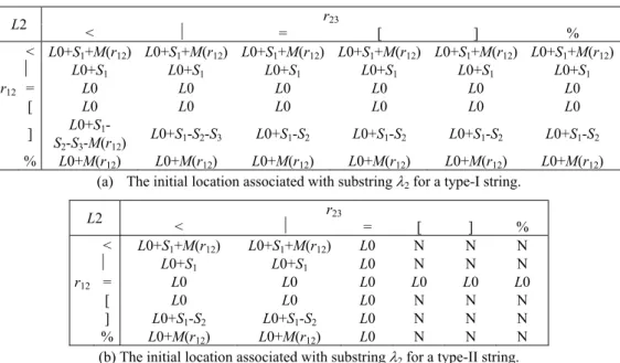
3.1.3 The initial locations
The initial locations associated with substrings λ1, λ2 and λ3 are the same as the lo-cations of o1, o2 and o1, respectively. The location of o1 is the same as the initial location associated with the original 3-object string. So, we onlyneed to compute the initial loca-tion associated with substring λ2. The initial location associated with substring λ2, L2, can be derived from Figs. 6 (a) and (b) for type-I and type-II strings, respectively. For a type-III string, the derived relation and metric information are the same as the original string. r23 L2 < ⏐ = [ ] % < L0+S1+M(r12) L0+S1+M(r12) L0+S1+M(r12) L0+S1+M(r12) L0+S1+M(r12) L0+S1+M(r12) ⏐ L0+S1 L0+S1 L0+S1 L0+S1 L0+S1 L0+S1 r12 = L0 L0 L0 L0 L0 L0 [ L0 L0 L0 L0 L0 L0 ] L0+S1- S2-S3-M(r12) L0+S1-S2-S3 L0+S1-S2 L0+S1-S2 L0+S1-S2 L0+S1-S2 % L0+M(r12) L0+M(r12) L0+M(r12) L0+M(r12) L0+M(r12) L0+M(r12) (a) The initial location associated with substring λ2 for a type-I string.
r23 L2 < ⏐ = [ ] % < L0+S1+M(r12) L0+S1+M(r12) L0 N N N ⏐ L0+S1 L0+S1 L0 N N N r12 = L0 L0 L0 L0 L0 L0 [ L0 L0 L0 N N N ] L0+S1-S2 L0+S1-S2 L0 N N N % L0+M(r12) L0+M(r12) L0 N N N
(b) The initial location associated with substring λ2 for a type-II string. Fig. 6. The initial location associated with substring λ2 for type-I and type-II string.
Now, let’s consider a type-I string 10(A7 <2 (B3 |C2)), where the subscript 10 is the initial location associated with the template object and the relations of r12 and r23 are “<” and “|”, respectively. We can derive the following substrings: ω1: (A7 <B3) from Fig. 2
(a), ω2: (B3 |C2) from Fig. 2 (b), and ω3: (A7 < C2) from Fig. 2 (c). The distance associ-ated with operator < in substring ω1 is equal to M(<2) = 2 from Fig. 4 (a), operator | in substring ω2 does not have metric information from Fig. 4 (b), and the distance associ-ated with operator < in substring ω3 is equal to M(<2) + SB = 2 + 3 = 5 from Fig. 4 (c).
The initial location associated with substring ω2 is equal to 10 + SA + M(<2) = 10 + 7 + 2 = 19 from Fig. 6 (a).
The relation and metric information between any two objects in a 3-object string can be derived from the tables as shown in Figs. 2 to 6. For a 3D C-string containing more than 3 objects, we need more inference rules and discuss them in following subsections. 3.2 Transitive Rules for the String with More Than 3 Objects
(TR-1) If r12 ∈ R, and r(i-1)i ∈ {“=”, “[“, “]”, “%”}, 2 < i ≤ n, and the first level of the 3D C-string is of type-I, the string will be in the form of L0(o1r12(o2r23(o3r34(…(o(n-1)r(n-1)n on)…)))). Let o′3 be (o3r34(…(o(n-1)r(n-1)non)…)). The string can be rewritten as L0(o1r12(o2 r23o′3)). So, we can get the following three substrings.
λ4: L0(o1r′12o2), where r′12 canbe derived from Fig. 2 (a),
λ5: L2(o2r23o′3), that is, L2(o2r23(o3r34(…(o(n-1)r(n-1)non)…))), where L2 can be derived from
Fig. 6 (a),
λ6: L0(o1r′13o′3), that is, L0(o1r′13(o3r34(…(o(n-1)r(n-1)non)…))), where r′13 can be derived from Fig. 2 (c).
For example, for a 3D C-string L0(A%(B](C[D))), we will have the following three
substrings: ω4: L0(A %B), ω5: L2(B](C[D)), and ω6: L0(A%(C[D)), where the metric
information is omitted. Because the substrings ω5 and ω6 are in the form of rule (TR-1), rule (TR-1) can be recursively applied to find every binary relation between the objects. (TR-2) If r(n-1)n ∈ {“<”, “|”, “|t”}, and r(i-1)i ∈ {“=”, “[“, “]”, “%”}, 1 < i < n, and the first level of the 3D C-string is of type-II, the string will be in the form of L0((o1r12(o2r23(… (o(n-2)r(n-2)(n-1)o(n-1))…)))r(n-1)non). Let o′2 be (o2r23(…(o(n-2)r(n-2)(n-1)o(n-1))…)). The string can be rewritten as L0((o1r12o′2)r(n-1)non). So, we will have the following three substrings.
λ7: L0(o1r12o′2 ), that is, L0(o1r12(o2r23(…(o(n-2)r(n-2)(n-1)o(n-1))…))),
λ8: L2(o′2 r′(n-1)non), that is, L2((o2r23(…(o(n-2)r(n-2)(n-1)o(n-1))…))r′(n-1)non), where r′(n-1)n and L2 can be derived from Fig. 3 (b) and Fig. 6 (b), respectively,
λ9: L0(o1r′1non), where r′1n can be derived from Fig. 3 (c).
For example, for a 3D C-string, L0((A[(B](C%D)))|E), we will have the following
three substrings: ω7: L0(A[(B](C%D))), ω8: L2((B](C%D))<E), and ω9: L0(A|E),
where the metric information is omitted. Substring ω7 is in the form of (TR-1), and sub-string ω8 is in the form of (TR-2), so (TR-1) and (TR-2) can be recursively applied to find every binary relation between the objects.
3.3 Distributive Rules
We have discussed the 3D C-strings with the form of nested parentheses in the pre-vious section. To infer the relations between the objects in the 3D C-strings of another form, we first consider a four-symbol string in the form of L0((o1r12 o2)r23(o3r34o4)). Let o′3 be (o3r34o4). The string can be rewritten as L0((o1r12o2)r23o′3 ) which is of type-II. So, we can have following three substrings: λ10: L0(o r o1 13 3′ ′) which is L0(o r o r o1 13′( 3 34 4)),λ11: L2(o 2
23 3)
r o′ ′ which is L2((o r o r o2 23′( 3 34 4)), and λ12: L0(o1r12o2).
Or, we can replace (o1r12o2) with o′2 . The string can be rewritten as L0(o′2 r23 (o3r34o4)) which is of type-I. So, we can have the following three substrings: λ13: L0(o r o2 23 3′ ′ ),that is,
0(( 1 12 2)23 3),
L o r o r o′ λ14: L2((o r o3 34 4), and λ15: L0(o r o′ ′2 24 4), that is, L0((o r o r o1 12 2)24 4′ ). After the distribution, we can easily apply the transitive rules to infer the relations between each pair of objects.
For example, for a 3D C-string, L0((A%B)<(C[D)), we can replace (A%B) with
2.
o′ The string can be written as L0(o′ <2 (C[D)) which is of type-I. So, we can have the following three substrings: ω10: L0(o′ <2 C) which is L0((A%B)<C), ω11: L0(o′ <2 D) which is L0((A%B)<D), ω12: L2(C[D). For the substrings ω10 and ω11, we can apply the transi-tive rules to infer the relations between the objects.
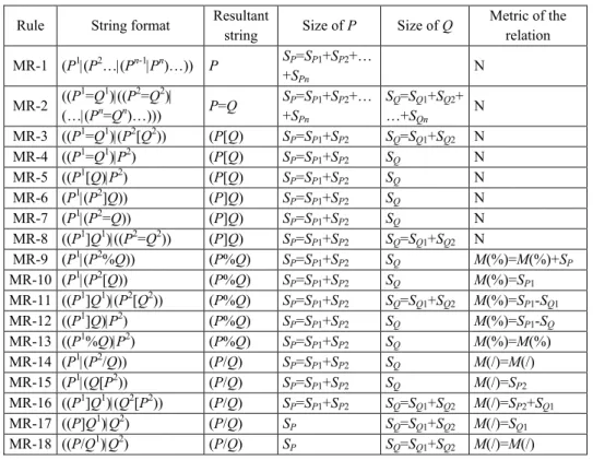
Table 2. The manipulation rules. Rule String format Resultant
string Size of P Size of Q
Metric of the relation MR-1 (P1|(P2…|(Pn-1|Pn)…)) P SP=SP1+SP2+… +SPn N MR-2 ((P 1=Q1)|((P2=Q2)| (…|(Pn=Qn)…))) P=Q SP=SP1+SP2+… +SPn SQ=SQ1+SQ2+ …+SQn N MR-3 ((P1=Q1)|(P2[Q2)) (P[Q) S P=SP1+SP2 SQ=SQ1+SQ2 N MR-4 ((P1=Q1)|P2) (P[Q) SP=SP1+SP2 SQ N MR-5 ((P1[Q)|P2) (P[Q) S P=SP1+SP2 SQ N MR-6 (P1|(P2]Q)) (P]Q) S P=SP1+SP2 SQ N MR-7 (P1|(P2=Q)) (P]Q) S P=SP1+SP2 SQ N MR-8 ((P1]Q1)|((P2=Q2)) (P]Q) SP=SP1+SP2 SQ=SQ1+SQ2 N MR-9 (P1|(P2%Q)) (P%Q) S P=SP1+SP2 SQ M(%)=M(%)+SP MR-10 (P1|(P2[Q)) (P%Q) S P=SP1+SP2 SQ M(%)=SP1 MR-11 ((P1]Q1)|(P2[Q2)) (P%Q) S P=SP1+SP2 SQ=SQ1+SQ2 M(%)=SP1-SQ1 MR-12 ((P1]Q)|P2) (P%Q) SP=SP1+SP2 SQ M(%)=SP1-SQ MR-13 ((P1%Q)|P2) (P%Q) S P=SP1+SP2 SQ M(%)=M(%) MR-14 (P1|(P2/Q)) (P/Q) S P=SP1+SP2 SQ M(/)=M(/) MR-15 (P1|(Q[P2)) (P/Q) S P=SP1+SP2 SQ M(/)=SP2 MR-16 ((P1]Q1)|(Q2[P2)) (P/Q) SP=SP1+SP2 SQ=SQ1+SQ2 M(/)=SP2+SQ1 MR-17 ((P]Q1)|Q2) (P/Q) SP SQ=SQ1+SQ2 M(/)=SQ1 MR-18 ((P/Q1)|Q2) (P/Q) S P SQ=SQ1+SQ2 M(/)=M(/)
3.4 Manipulation Rules
In the 3D C-string representation, the subobjects would only be present in the rela-tion of part_overlap, “/”. It is necessary for us to manipulate (merge) the subobjects. The manipulation rules are used to merge together the subobjects in one string (or substring). The integration rules in section 3.4 are used to merge together the subobjects in two strings (or substrings). We present 18 manipulation rules in this subsection as shown in Table 2 and 21 integration rules in the next subsection. In Table 2, the first column shows the name of a rule, and the second column presents the original string format, where Pi, 1
≤ i ≤ n, are the subobjects of P. The merged result is listed in the third column, and the size of P or Q and metric of the relation are shown in the remaining columns, where ‘N’ denotes that there is not metric information for those cases, and SP denotes the size of
object P.
We do not use operator / in the 3D C-string representation; however, we do use op-erator / in the inference process. The distance associated with opop-erator /, P/d Q, is equal
to the distance between the x- (y- or time-) projection of object P and that of objectQ, where d = EBx(P) – BBx(Q) (d = EBy(P) – BBy(Q), or d = EBtime(P) – BBtime(Q)).
These manipulation rules are used to merge the subobjects in a string together. The location of merged object keeps unchanged. Let’s consider an example as follows, where objects A and B are partitioned into several subobjects in a string, (A2 |(A2 |(((A4 ]B2)| ((A2 =B2)|(A2 =B2)))|(B2 |B2)))). We can merge objects A and B together in the follow-ing steps. (A2 |(A2 |(((A4 ]B2)|((A2 =B2)|(A2 =B2)))|(B2 |B2)))) (MR-1) (A2 |(A2 |(((A4 ]B2)|((A2 =B2)|(A2 =B2)))|B4))) (MR-2) (A2 |(A2 |(((A4 ]B2)|(A4 =B4))|B4))) (MR-8) (A2 |(A2 |((A8 ]B6)|B4))) (MR-17) (A2 |(A2 |(A8 /6 B10))) (MR-14) (A2 |(A10 /6 B10)) (MR-14) (A12 /6 B10)
where the underline parts will be merged together in the next step. Finally, the relation between A and B is (A12 /6 B10).
3.5 Integration Rules
The integration rules are used to merge the subobjects in several substrings together. There are 21 integration rules in total as shown in Table 3. In Table 3, the first column shows the name of a rule, the second and third columns present the two substrings to be combined. The integrated result is listed in the next column, and the size of P or Q and metric of relation are shown in the remaining columns, where “N” denotes that there is not metric information for those cases, M1 and M2 are the metric information of the op-erators in String 1 and String 2, respectively.
Table 3. The integration rules.
Rule String 1 String 2 Resultant string Size of P Size of Q Metric of the relation IR-1 (P1<Q) (P2<Q) (P<Q) S P=SP1+SP2 SQ M(<)=Min(M1(<), M2(<)) IR-2 (P<Q1) (P<Q2) (P<Q) S P SQ=SQ1+SQ2 M(<)=Min(M1(<), M2(<)) IR-3 (P1<Q) (P2|Q) (P|Q) S P=SP1+SP2 SQ N IR-4 (P|Q1) (P<Q2) (P|Q) S P SQ=SQ1+SQ2 N IR-5 (P1=Q1) (P2=Q2) (P=Q) S P=SP1+SP2 SQ=SQ1+SQ2 N IR-6 (P1=Q1) (P2[Q2) (P[Q) S P=SP1+SP2 SQ=SQ1+SQ2 N IR-7 (P1=Q) (Q|P2) (P[Q) S P=SP1+SP2 SQ N IR-8 (P1[Q) (Q<P2) (P[Q) S P=SP1+SP2 SQ N IR-9 (P1<Q) (P2]Q) (P]Q) S P=SP1+SP2 SQ N IR-10 (P1|Q) (P2=Q) (P]Q) S P=SP1+SP2 SQ N IR-11 (P1]Q1) (P2=Q2) (P]Q) S P=SP1+SP2 SQ=SQ1+SQ2 N IR-12 (P1<Q) (P2%Q) (P%Q) S P=SP1+SP2 SQ M(%)=M(%)+SP1 IR-13 (P1|Q) (P2[Q) (P%Q) S P=SP1+SP2 SQ M(%)=SP1 IR-14 (P1]Q1) (P2[Q2) (P%Q) S P=SP1+SP2 SQ=SQ1+SQ2 M(%)=SP1-SQ1 IR-15 (P1]Q) (Q|P2) (P%Q) S P=SP1+SP2 SQ M(%)=SP1-SQ IR-16 (P1%Q) (Q<P2) (P%Q) S P=SP1+SP2 SQ M(%)=M1(%) IR-17 (P1<Q) (P2/Q) (P/Q) S P=SP1+SP2 SQ M(/)=M2(/) IR-18 (P1|Q) (Q[P2) (P/Q) S P=SP1+SP2 SQ M(/)=SP2 IR-19 (P1]Q1) (Q2[P2) (P/Q) S P=SP1+SP2 SQ=SQ1+SQ2 M(/)=SP2+SQ1 IR-20 (P]Q1) (P|Q2) (P/Q) S P SQ=SQ1+SQ2 M(/)=SQ1 IR-21 (P/Q1) (P<Q2) (P/Q) S P SQ=SQ1+SQ2 M(/)=M1(/)
These integration rules can be used to merge the subobjects in several substrings together. For example, object A is partitioned into two subobjects: 1
2
A and 2 3
A , and B is partitioned into three subobjects: 1
3
B , 2 3
B , and 3 4
B . Those subobjects appear in six sub-strings: ω13: (A B12| 13), ω14: (A32=B13), ω15: (A B12| 32), ω16: (A32<3B32), ω17: (A12<7B43), and ω18: (A32<4B43). We can use the integration rules to derive the relation between ob-jects A and B in the following steps.
(IR-10) Integrate ω13 and ω14 to ω19: (A1,25 ] )B13 (IR-3) Integrate ω15 and ω16 to ω20: (A51,2|B32) (IR-1) Integrate ω17 and ω18 to ω21: (A51,2<4B43) (IR-20) Integrate ω19 and ω20 to ω22: (A51,2/3B1,26 )
(IR-21) Integrate ω21 and ω22 to ω23: (A51,2/3 10B1,2,3) => (A5 /3 B10)
where a superscript denotes a sequence number of the subobject and a subscript denotes the size of a subobject. Finally, the relation between A and B is (A5 /3 B10).
3.6 Relation Derivation Algorithm
After presenting the inference rules, we propose the relation derivation algorithm to infer the spatio-temporal relations between the objects in a 3D C-string. Assume that there are k levels of template objects and m objects in a given 3D C u-string (v- or
t-string), and those objects are numbered from 1 to m. For each subobject of object i, we assign a sequence number to it. For example, if object i is cut into three subobjects, those subobjects are numbered as i.1, i.2 and i.3, where 1, 2, and 3 are the sequence numbers. The relation derivation algorithm can infer a list of relations between any two objects in a given 3D C u-string (v- or t-string). The relation derivation algorithm is described in detail in Fig. 7.
Algorithm relation derivation
Input: a 3D C-string u-string (v- or t-string). Output: ϕ, the relations between any two objects.
1. Let the relation list ϕ be null and the string list ψ be null. 2. Assign a sequence number to each subobject of object i. 3. Add the input string to ψ.
4. while (ψ is not empty) do
5. Remove the first string η from ψ. 6. if (η contains subobjects) then
7. Apply the manipulation rules to merge the subobjects in η. 8. end if
9. Apply the transitive or distributive rules to η. 10. for each generated substring ρ do
11. if (ρ contains only two objects and is not in ϕ) then 12. Append ρ to ϕ. 13. elseif (ρ is not in ψ) 14. Append ρ to ψ. 15. end if 16. end for 17. end while
18. Apply the integration rules to the strings in ϕ.
Fig. 7. Relation derivation algorithm.
In this algorithm, we process a template object for each loop in steps 4-17. In steps 6-8, if η contains subobjects, we use the manipulation rules to merge the subobjects in η. Then, we apply the transitive or distributive rules to infer the relations between objects in step 9. In steps 10-16, if the generated substring ρ contains only two objects, collect it into ϕ; otherwise, collect it into ψ. The substrings in ψ need to be processed in the later steps. In the last step, we apply the integration rules to merge the subobjects in ϕ. Lemma 1 For a 3D C u- (v-, or t-) string, the time complexity of the relation derivation algorithm is bounded to O(k2+ c × m × t + c2 × t2), wherec is the maximum number of cuttings among all individual objects, m is the number of objects, t is the number of cut objects, k is the number of levels of the template object in the input string.
Theorem 1 For a 3D C-string, the time complexity of the relation derivation algorithm is bounded to O(k2 + c × m × t + c2 × t2), where c is the maximum number of cuttings
among all individual objects; m is the number of objects in the input string; k is the maximum value of k1, k2, k3; k1, k2, k3 are the numbers of levels of the template objects in the u-, v-, and t-strings, respectively; and t is the maximum value of t1, t2, t3; t1, t2, t3 are the numbers of cut objects in u-, v-, t-strings, respectively.
Let’s consider the example as shown in Fig. 1. The u-string of the video is 0(((C2↑2,1 =D2↑2,1)|A4)<2 B4), which is of type-II. We can use the transitive rules to generate the following three substrings: ω24: 0((C2↑2,1 =D2↑2,1)|A4), ω25: 2(A4 <2 B4), and ω26: 0((C2↑2,1 =D2↑2,1)<6 B4).
The relations associated with substrings ω25 and ω26 can be derived from Figs. 3 (b) and (c). The metric information and initial location of substring ω25can be derived from Fig. 5 (b) and Fig. 6 (b), and the metric information of substring ω26 can be derived from Fig. 5 (c). That is, M(r13) = S2 + M(r23) = 4 (the size of object A) + 2 (metric of operator “<”) = 6. Likewise, we can apply the same rule to substrings ω24 and ω26. From substring ω24, we can obtain the substrings ω27: 0(C2↑2,1 =D2↑2,1), ω28: 0(D2↑2,1 |A4) and ω29: 0(C2↑2,1 |A4). From substring ω26, we can obtain the substrings ω30: 0(C2↑2,1 =D2↑2,1), ω31: 0(D2↑2,1 <6 B4) and ω32: 0(C2↑2,1 <6 B4). Hence, we can get all the relations between each pair of objects in the x dimension.
Similarly, from v-string (D1↑0,1 <1 (C1↑0,1 <1 (A4 =B4))) we can derive the relation between each pair of objects in the y dimension. First of all, we apply the transitive rules to the v-string and obtain the following three substrings: ω33: 0(D1↑0,1 <1 C1↑0,1), ω34: 2(C1↑0,1 <1 (A4 =B4)), and ω35: 0(D1↑0,1 <3 (A4 =B4)). Second, we can obtain the following substring: ω36: 2(C1↑0,1 <1 A4), ω37: 4(A4 =B4) and ω38: 2(C1↑0,1 <1 B4) from ω34, and ω39: 0(D1↑0,1 <3 A4), ω40: 4(A4 =B4) and ω41: 0(D1↑0,1 <3 B4) from ω35. Similarly, from t-string (A6 =B6 =C6 =D6), that is of type-III, we can easily derive the relations between the ob-jects, namely, the relation between each pair of objects in the time dimension is “=”. That is, ω42: 0(A6 =B6), ω43: 0(A6 =C6), ω44: 0(A6 =D6), ω45: 0(B6 =C6), ω46: 0(B6 =D6), and ω47: 0(C6 =D6).
From substrings ω25, ω37 and ω42, we know that the relations between objects A and B are 2(A4 <2 B4) in the x dimension, 4(A4 =B4) in the y dimension and 0(A6 =B6) in the time dimension. So, we can find that objects A and B are both still, disjoined, and of the same size. From the substrings ω27, ω33 and ω47, we know that the relations between ob-jects C and D are 0(C2↑2,1 =D2↑2,1)in the x dimension,0(D1↑0,1 <1 C1↑0,1) in the y dimen-sion and 0(C6 =D6) in the time dimension. So, we can find that objects C and D are mov-ing at the same speed and object D is one unit below object C in the y dimension.
Let’s consider another example. We add six more frames to the video shown in Fig. 1, where a moving car, E, has the same initial location and velocity as object C in frames 7~12. Hence, the corresponding 3D C-string for the video is shown as follows: u-string: (((C2↑2,1 =D2↑2,1 =E2↑2,1)|A4)<2 B4), v-string: (D1↑0,1 <1 ((C1↑0,1 =E1↑0,1)<1 (A4 =B4))), t-string: ((A12 =B12) = ((C6 =D6)|E6)). Then, we can infer the relation between objects C and E and obtain the following relations: 0(C2↑2,1 =E2↑2,1) in the x dimension, 0(C1↑0,1 = E1↑0,1) in the y dimension, and 0(C6 |E6) in the time dimension. Both objects C and E have the “=” relation and the same velocity in the x and y dimensions. In the time dimen-sion, both objects have the same size and “|” relation. That is, object E appears right after object C disappears. Therefore, with these rules, a user can easily derive the relations between the objects in a video represented by the 3D C-string.
4. AN APPLICATION
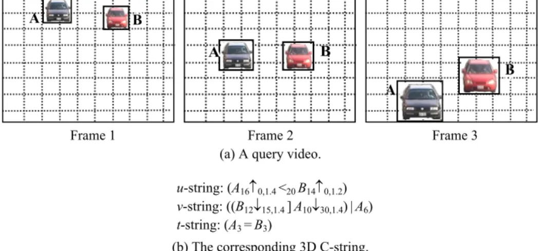
In this section, we demonstrate a video query example to show the effectiveness of our video algebra. The query video V of an overtaking event is shown in Fig. 8, where car A is overtaking car B. The query video is shown in Fig. 8 (a) and the corresponding 3D C-string is shown in Fig. 8 (b).
A A B B B A A B B AA B
Frame 1 Frame 2 Frame 3 (a) A query video.
u-string: (A16↑0,1.4 <20 B14↑0,1.2)
v-string: ((B12↓15,1.4 ]A10↓30,1.4)|A6)
t-string: (A3 =B3)
(b) The corresponding 3D C-string. Fig. 8. A video query example of an overtaking event.
u-string: (A42↑0,1.4 |((D45 ]B12↑0,1.2)|(C38↑0,1.2 [B28)))
v-string: ((B62↓32,1.6 ]A20↓45,1.8)|((A40 =C40↓30,1.5)]D30))
t-string: ((A60 =B60)](C50 ]D1))
Fig. 9. The 3D C-string of the matched video.
To find the videos similar to V from a database, we first choose the database videos that contain more than one car object. For example, let’s consider a database video containing four car objects A, B, C, and D, and its corresponding 3D C-string is shown in Fig. 9.
Next, from the u-string, we can use the video algebra to infer the relation between each pair of objects in the x dimension, and obtain the following six substrings, ω48: 0(A42↑0,1.4 <33 B40↑0,1.2),ω49: 0(A42↑0,1.4 <45 C38↑0,1.2), ω50: 0(A42↑0,1.4 |D45), ω51: 33(B40↑0,1.2 /28 C38↑0,1.2), ω52: 42(D45 /12 B40 ↑0,1.2), and ω53: 42(D45 |C38↑0,1.2).
Similarly, from the v-string, we can derive the relation for each pair of objects in the y dimension, and obtain the following six substrings, ω54: 0(B62↓32,1.6 /20 A60↓45,1.8), ω55: 62(A60↓45,1.8 ]C40↓30,1.5), ω56: 62(A60↓45,1.8 ]D30), ω57: 0(B62↓32,1.6 |C40↓30,1.5), ω58: 0(B62↓32,1.6 <10 D30), and ω59: 62(C40↓30,1.5)]D30). From t-string, we can derive the relation for each pair of objects in the time dimension, and obtain the following six substrings, ω60: 0(A60 = B60), ω61: 0(A60 ]C50), ω62: 0(A60 ]D1), ω63: 0(B60 ]C50), ω64: 0(B60 ]D1), and ω65: 10(C50 ] D1).
According to the overtaking event between objects A and B in the query video, we can derive the “<” (disjoin) relation in the x dimension, the “/” (partly-overlap) relation in the y dimension, the “=” (equal) relation in the time dimension, and object A with a higher velocity than object B in the y dimension. In the video shown in Fig. 9, we can find that the relations between objects A and B are ω48: 0(A42↑0,1.4 <33 B40↑0,1.2) in the x dimension, ω54: 0(B62↓32,1.6 /20 A60↓45,1.8) in the y dimension, and ω60: 0(A60 =B60) in the time dimension, and object A with a higher velocity than object B in the y dimension. Thus, we can retrieve the database video similar to the query video and the database video is showed in Fig. 10.
A B A B C A B C
Frame 1 Frame 20 Frame 30
A B C A B C B A C D
Frame 40 Frame 50 Frame 60 Fig. 10. The matched video.
5. CONCLUSIONS
The video content management has attracted increasing attention in recent years. We have proposed a new spatio-temporal knowledge structure, called 3D C-string, to represent the spatio-temporal relations between the objects in a video and to keep track of the motions and size changes of the objects. In this paper, we propose a video algebra to infer the spatio-temporal relations between the objects in a video represented by the 3D C-string. The algebra contains four kinds of rules, namely, transitive, distributive, manipulation, and integration rules. By using those rules, all the binary relations between the objects in a video can be derived from a given 3D C-string. These rules provide us the theoretic basis for spatio-temporal reasoning and video query inference. How to ex-pand the reasoning result to generate the high-level semantics and to support high-level semantic video queries is worth further study.
REFERENCES
1. S. F. Chang, W. Chen, H. Meng, H. Sundaram, and D. Zhong, “A fully automatic content-based video search engine supporting multi-object spatio-temporal queries,” IEEE Transactions on Circuit Systems and Video Technology, Vol. 8, 1998, pp. 602-615.
2. M. R. Naphade, I. V. Kozintsev, and T. S. Huang, “Factor graph framework for se-mantic video indexing,” IEEE Transactions on Circuits and Systems for Video Tech-nology, Vol. 12, 2002, pp. 40-52.
3. C. W. Ngo, T. C. Pong, and H. J. Zhang, “Motion analysis and segmentation through spatio-temporal slices processing,” IEEE Transactions on Image Processing, Vol. 12, 2003, pp. 341-355.
4. H. Yang, L. Chaisorn, Y. Zhao, S. Neo, and T. Chua, “VideoQA: question answering on news video,” in Proceedings of ACM International Conference on Multimedia, 2003, pp. 632-641.
5. C. C. Lo, S. J. Wang, and L. W. Huang, “Video retrieval using successive modular operations on temporal similarity,” Computer Standards and Interfaces, Vol. 26, 2004, pp. 317-328.
6. C. G. M. Snoek and M. Worring, “Multimedia event based video indexing using time intervals,” IEEE Transactions on Multimedia, Vol. 7, 2005, pp. 638- 647.
7. S. K. Chang, Q. Y. Shi, and C. W. Yan, “Iconic indexing by 2D strings,” IEEE Tran- sactions on Pattern Analysis and Machine Intelligence, Vol. 9, 1987, pp. 413-429. 8. S. K. Chang, E. Jungert, and Y. Li, “Representation and retrieval of symbolic
pic-tures using generalized 2D strings,” in Proceedings of SPIE on Visual Communica-tions and Image Processing, 1989, pp. 1360-1372.
9. E. Jungert and S. K. Chang, “An algebra for symbolic image manipulation and transformation,” Visual Database Systems, North-Holland: Elsevier Science Pub-lishers B.V., 1989.
10. S. Y. Lee and F. J. Hsu, “2D C-string: a new spatial knowledge representation for image database system,” Pattern Recognition, Vol. 23, 1990, pp. 1077-1087. 11. S. Y. Lee and F. J. Hsu, “Picture algebra for spatial reasoning of iconic images
rep-resented in 2D C-string,” Pattern Recognition Letters, Vol. 12, 1991, pp. 425-435. 12. S. Y. Lee and F. J. Hsu, “Spatial reasoning and similarity retrieval of images using
2D C-string knowledge representation,” Pattern Recognition, Vol. 25, 1992, pp. 305-318.
13. P. W. Huang and Y. R. Jean, ”Using 2D C+-string as spatial knowledge representa- tion for image database systems,” Pattern Recognition, Vol. 27, 1994, pp. 1249-1257. 14. P. W. Huang and Y. R. Jean, “Spatial reasoning and similarity retrieval for image
database systems based on RS-strings,” Pattern Recognition, Vol. 29, 1996, pp. 2103-2114.
15. F. J. Hsu, S. Y. Lee, and B. S. Lin, “2D C-trees spatial representation for iconic im-age,” Journal of Visual Languages and Computing, Vol. 10, 1999, pp. 147-164. 16. Y. I. Chang, H. Y. Ann, and W. H. Yeh, “A unique-ID-based matrix strategy for
efficient iconic indexing of symbolic pictures,” Pattern Recognition, Vol. 33, 2000, pp. 1263-1276.
ma-trix strategy for efficient iconic indexing of symbolic pictures,” Pattern Recognition Letters, Vol. 22, 2001, pp. 657-666.
18. G. Petraglia, M. Sebillo, M. Tucci, and G. Tortora, “Virtual images for similarity retrieval in image databases,” IEEE Transactions on Knowledge and Data Engi-neering, Vol. 13, 2001, pp. 951-967.
19. Y. I. Chang, B. Y. Yang, and W. H. Yeh, “A bit-pattern-based matrix strategy for efficient iconic indexing of symbolic pictures,” Pattern Recognition Letters, Vol. 24, 2003, pp. 537-545.
20. A. J. T. Lee and H. P. Chiu, “2D Z-string: A new spatial knowledge representation for image databases,” Pattern Recognition Letters, Vol. 24, 2003, pp. 3015-3026. 21. K. Shearer, S. Venkatesh, and D. Kieronska, “Spatial indexing for video databases,”
Journal of Visual Communication and Image Representation, Vol. 7, 1996, pp. 325-335.
22. K. Shearer, D. Kieronska, and S. Venkatesh, “Resequencing of video using spatial indexing,” Journal of Visual Languages and Computing, Vol. 8, 1997, pp. 193-214. 23. F. J. Hsu, S. Y. Lee, and B. S. Lin, “Video data indexing by 2D C-trees,” Journal of
Visual Languages and Computing, Vol. 9, 1998, pp. 375-397.
24. Y. K. Chan and C. C. Chang, “Spatial similarity retrieval in video databases,” Jour- nal of Visual Communication and Image Representation, Vol. 12, 2001, pp. 107-122. 25. C. C. Liu and A. L. P. Chen, “3D-list: a data structure for efficient video query
proc-essing,” IEEE Transactions on Knowledge and Data Engineering, Vol. 14, 2002, pp. 106-122.
26. A. J. T. Lee, H. P. Chiu, and P. Yu, “3D C-string: a new spatio-temporal knowledge structure for video database systems,” Pattern Recognition, Vol. 35, 2002, pp. 2521-2537.
Anthony J. T. Lee (李瑞庭) received the B.S. degree from National Taiwan University, Taiwan, in 1983. He got the M.S. and Ph.D. degree in Computer Science from University of Illinois at Urbana-Champaign, U.S.A., in 1990 and 1993, respectively. In August 1993, he joined the Department of Information Manage-ment at National Taiwan University and he is now a professor. His current research interests include multimedia databases, temporal and spatial databases, and data mining.
Ping Yu (余平) is currently a Ph.D. candidate in the De-partment of Information Management, National Taiwan Univer-sity, Taipei, Taiwan R.O.C. He received the B.S. degree from Chung Cheng Institute of Technology, Taiwan, in 1988, and the M.S. degree from National Defense Management College, Tai-wan, in 1994. His current research interests include multimedia databases, temporal and spatial databases.
Han-Pang Chiu (邱漢邦) is currently a Ph.D. candidate in the Learning and Intelligent Systems group at the Computer Sci-ence and Artificial IntelligSci-ence Laboratory at Massachusetts In-stitute of Technology, U.S.A. He received his BBA degree from National Taiwan University, Taiwan, in 1999, and his MBA de-gree from the Department of Information Management, National Taiwan University, in June 2001. His current research interests include computer vision and machine learning. He is focusing on the topics of learning in visual perception, 3D object class recog-nition, and wide baseline stereo matching. His doctoral research is part of the Transfer Learning project supported by the Defense Advanced Research Projects Agency (DARPA).
Hsiu-Hui Lin (林秀慧) is currently a Ph.D. candidate in the Department of Information Management, National Taiwan Uni-versity, Taipei, Taiwan, R.O.C. She received the B.S. degree from Department of Computer Science and Information Engi-neering, National Taiwan University, in 1988, and the M.S. de-gree from Department of Computer Science and Information En-gineering, National Taiwan University, in 1991. Her current re-search interests include multimedia databases, and digital copy-right management.