行政院國家科學委員會補助專題研究計畫成果報告
非同步處理器模擬器的設計與資料危障問題的研究
The implementation of simulator for asynchronous processor and the
study of data hazards
計畫類別:
a個別型計畫 □整合型計畫
計畫編號:NSC 90-2213-E-009-155-
執行期間:90 年 08 月 01 日 至 91 年 07 月 31 日
計畫主持人:陳昌居 副教授
共同主持人:
本成果報告包括以下應繳交之附件:
□赴國外出差或研習心得報告一份
□赴大陸地區出差或研習心得報告一份
□出席國際學術會議心得報告及發表之論文各一份
□國際合作研究計畫國外研究報告書一份
執行單位:國立交通大學資訊工程學系
中
華
民
國
91 年
12 月
30 日
行政院國家科學委員會專題研究計畫成果報告
非同步處理器模擬器的設計與資料危障問題的研究
The implementation of simulator for asynchr onous pr ocessor and the
study of data hazar ds
計畫編號:NSC 90-2213-E-009-155
執行期限:90 年 8 月 01 日至 91 年 07 月 31 日
主持人:陳昌居
國立交通大學資訊工程學系
E-mail: cjchen@csie.nctu.edu.tw
Abstr act
Asynchronous processors have become a new direction of modern architecture research these years. To compare the improvement of different approaches without designing a real ASIC, we need a code-based simulator. That’s the reason we want to design SimAsync, an asynchronous processor simulator, for researches in asynchronous architectures. The simulator tools are based on SimpleScalar[1], a public simulator of modern microprocessors, and contain a complete description of the target processor architecture, and many details about the internals of the tools. We also give the discussion of data hazards related to asynchronous design. 摘要 最近幾年非同步處理器成為當今計算機架構 研究的新方向。為了在不需要真實積體電路情 形下,來比較不同方法所做的改善,我們需要 一個模擬器。此即為我們設計 SimAsync 的原 因,它是用來做非同步架構研究的非同步處理 器的模擬器。此模擬器是根據 SimpleScalar 工 具而製作,這個工具是一個公開的現代處理器 之模擬器,它包含了完整的目標處理器架構的 描述,以及其套件內部的詳細說明。我們也討 論有關於非同步設計的資料危障。
1. Introduction
Asynchronous architecture is a new research topic in computer architecture. There are several asynchronous processor prototypes announced in the past years, but we cannot find any asynchronous processor simulator for the study and research. We really need a simulator to investigate this new architecture and to measure improvements we are trying to do before it is implemented.As systems grow increasingly large and complex, clock can cause big problems with
clock skew. It means a timing delay between several parts of system and may introduce logical error. To avoid clock skew, the clock tree should be placed early and several routing algorithms are needed. It increases the difficult of circuit design and we need more silicon area in the system so that the cost of each die is increased, too. It also leads to more power dissipation and overheating, and this kind of processors won’t be suitable for handing devices and mobile computing in the modern applications. However, all of the usual improvements, the clock skew will be more serious. There exists some bottleneck in the synchronous designs in the near future.
To overcome such limitations, computer architecture researchers are actively considering asynchronous processor design. Instead of global clock, in an asynchronous architecture, each stage communicates with each other by some protocol. Without global clock, asynchronous architecture can permit modular design, exhibits the average performance of all components rather than worst-case performance of single component, and reduced power dissipation [2]. In the ideal situation, asynchronous processors have the mentioned advantages above. But in real world, asynchronous designs suffer from poor performance. Some researches figure out that some problems, like branch miss penalty and data dependency, cannot be solved easily in asynchronous environment.
The power dissipation reduction is not as good as expected, neither. Because the additional control logics between each stage also need power, the implementation of control logics should be more refined. On the other hand, reduce the units needed to process the instruction can decrease the power consumption, too. To do this, we need to classify the instruction types and to refine the control protocol. Shut down the
functional unit when it will not be used recently is also a possible solution. But we have to design an effective way to control the action of shutting down and waking up.
We design an asynchronous processor simulator to provide researchers an open general platform. We believe that through the simulator, more high quality researches can easily be achieved.
In order to study various architectures of asynchronous processors, a software simulator is needed first. The proposed simulator, SimAsync, is developed for the reason to provide a general architecture for asynchronous processor research. Following sections contain more information about the implementation of tool set for the simulator. In next section, we describe some related works about asynchronous processors and SimpleScalar. The design measures are described in section 3. In section 4, we introduce SimAsync architecture. In section 5, the implementation details and verification results are presented. A brief conclusion and future work are provided in section 6.
2. Related Wor k
In this section, we describe someresearches about asynchronous architectures and some proceeding plans of asynchronous
processors. SimpleScalar, the basis of SimAsync, is also included. At the last, we talk about the difficult problems of designs of asynchronous processors.
2-1. Micr opipelines
Sutherland[3] described an architecture named “Micropipelines”, which is an event-driven elastic pipeline. Sutherland introduced many event-driven logics and storage elements. Either rising or falling transition of signal is called an event and has the same meaning to circuits. He also announced how event control the actions of the whole pipeline. Data transfer between two stages is using two-phase bundled data interface. First, the sender puts valid data on data wires and then produces a “Request” event. After that, the receiver accepts the data and then produces an “Acknowledge” event. Data must be bundled with the “Request” control line so as to avoid the error occurs. In Figur e 1 and Figur e 2, the stages exchange data with each other through the
protocol.
It simply figures out how to use protocol to control the pipeline instead of traditional clock. SimAsync can support micropipelines, and it increases ILP.
2-2. Micr onets
D. K. Arvind et al. [4] defined a model for decentralising control in asynchronous processor architectures. Micronets proposed by them describes how a control unit control distributed functional units and gain the advantage through spatial concurrency in microagents within one stage.
Assume an execution unit in a traditional pipeline. In Figur e 3, there are three function units in the execution unit: shifter, multiplier and ALU. In Figur e 4, there are two types of instructions. Instructions of Type A needs only the shifter and the ALU, called set 1, to complete their calculation. And instructions of Type B needs them all, called set 2.
In traditional clock-driven pipeline, the clock rate is determined by the slowest stage, usually the execution unit. Other stages which finish their work early have to wait until the slowest stage finish its job. See the pipeline part in Figur e 5, it wastes too much time in waiting under clock-driven pipeline.
In micropipeline, the stages are event-driven, and it never needs a global clock. Each stage finishes its job and then starts next job as early as possible. Sometimes a stage needs to wait until the FIFOs have empty slots. See the
micropipeline part in Figur e 5, however, if the time each stage needs is fixed, the performance will be limited by the slowest stage, too.
Microagents, announced in micronets, mean that each function unit in each stage can communicate with other function unit. Instructions do not have to waste time in microagents they don’t need. So when Type A instructions are executed, they only need set 1 function units in execution unit. Similarly, Type B instructions need set 2 only. Control unit simply keeps the occupancy of each microagent and issues next instruction when its microagents are all free. In micronets, we will gain the benefit from multiple function units. In this case, if we have two shifters and two ALUs, we can issue Type A instructions without waiting. See the micronet part in Figur e 5, it is the mean to improve ILP in asynchronous architectures.
This release of SimAsync can’t support micronet but we support multiple function units.
2-3. AMULET [5, 6, 7, 8, 9]
AMULET, developed in the University of Manchester, actually is the most famous plan of implementation of asynchronous ARM architectures. The first release of AMULET is announced in 1994. This release proved the possibility to design an asynchronous processor. And this design method indeed provides the advantage that it can be implemented modularly.
On the other hand, AMULET 1 was suffered from the poor performance. Compared with the similar synchronous design, ARM 6, AMULET 1 needs more transistors and completes the benchmark programs slower and the worst, consumes more power. After some reasonable analysis, they believed that data dependency is the major part to influence the performance. In AMULET 1, when data dependency occurs, they simply stall the register access through locking the destination register. The locking mechanism offered nothing to improve performance. To attain better operation ability, we need some algorithms like result forwarding to solve the data dependency. It is nature in synchronous designs but hard in asynchronous environment. Many related researches are still in progress. This is one of the
reasons we want to design an asynchronous processor simulator. If we simulate the design before implementing, we can realize that locking mechanism is not suitable for asynchronous designs, and we can save the efforts.
To reduce the gate count, AMULET 1 research group have to improve latch circuits and change the communication protocol to four-phase bundled-data communication can be helpful to simplify the design. Figur e 6 shows timing diagram of this design.
After these improvements, AMULET 2 indeed achieved the similar performance level of synchronous designs. To compare with ARM 810, using the same CMOS process, AMULET 2 has better power efficiency. The latest version of AMULET is release 3.
2-4. SimpleScalar
SimpleScalar[1] is a simulation tool set that offers both detailed and high-performance simulation of modern microporcessors. It is based on MIPS-IV architecture, written in C language, and supports most platforms (Linux/Win32/Unix/FreeBSD/… ..).
SimpleScaler defines its own instruction set. The tool set also provide debugger, compiler, and pipeline status recorder. There are five execution-driven processor simulators in the tool set. Range from an extremely fast functional simulator to detailed, out-of-order issue, superscalar processor simulator that supports non-blocking caches and speculative execution. It is a load/store and two-source architecture. Only load/store instructions can access memory directly and there are at most two source operands for each instruction. It also defines both little-endian and big-endian versions of the architecture, so researchers can use the version that matches the endianess of any given host machine.
2-5. Ar duous Pr oblems of Asynchr onous Pr ocessor s Designs
In this section, we will discuss some difficult problems in asynchronous systems. Some of them have a general solution, and others still need better solutions.
2-5-1. Br anching [2]
Whether asynchronous or not, processors can reduce the branch penalty by one of five techniques: locking the pipeline, predict not-taken, predict taken, a branch prediction
algorithm, or delay slots.
To flush the mis-prefetch instructions is easy in synchronous processors, because the branch delay is fixed and known. However, in asynchronous processors, we have no idea about how many instructions fetched after the branch since the fetch unit fetch as many instruction as it could before the mis-prediction.
One technique to solve the problem is to bundle a “color-bit” with each fetched
instruction. All instructions have the same color until a branch encountered. At this point, the color changed and successive instructions have the different color. When mis-prediction is happened, the instructions which that have the wrong color are simply moved from the pipeline such that we will not commit the mis-prefetched instructions.
In our simulator, we simply flush all instructions succeed the mis-predicted branch.
2-5-2. Exception or Inter r upt Handling [2]
Hardware interrupts occur at random with internal control operations of the processors. Therefore, a metastability problem will be happened. In synchronous processors, the metastability is nearly eliminated through a series of flip-flops that the global clock regulates. However, the metastability is still never entirely eliminated from synchronous systems and the possibility increases with the clock frequency.
In asynchronous processors, the metastablity may be worse because there is no global clock to synchronize each functional unit [9]. We cannot know precise status of each functional unit when a hardware interrupt happened. What is lucky is that the nature of the asynchronous designs is easy to handle the interrupt processing mechanism. More design issues should be concerned as considering the interrupt handling.
We don’t support the exception handling in this release of our simulator.
2-5-3. Data For war ding
As we know, the register locking mechanism cannot make the performance better. We need some procedures like data forwarding to reduce the time to wait until the source data available. Naturally, data forwarding have to compare the destination register in the commit stage and the source registers in the decode stage. If the names are the same, data can be forwarded to the decode stage. However, “comparison” means that synchronization is needed between the two stages. It will increase the complexity of pipeline controls. Other algorithms, like scoreboard and reorder buffer, may be work. We still need to consider the complexity of implementation the algorithms. More investigations are needed to improve the solution.
In SimAsync, we try to solve this problem with a reorder buffer. This trial is just to provide a method and to implement it needs more analysis.
2-5-4. Communication with Off-chip Memor y
In synchronous systems, there is a global clock inside the core chip. Thus communication with off-chip memory is straightforward through a frequency divider. In asynchronous systems, arbitration or synchronization is needed to communicate with the off-chip memory with a fixed frequency. Synchronization means that the faster unit must slow down to wait the slower unit. It is clear that synchronization is not an efficient solution since it will influence the performance. However, arbitration is not always reliable so that many mechanisms need to be implemented to make sure that the failure is rarely to happen. To design an arbiter whose probability of failure is enough low to be unimportant will be a hot issue.
We ignore this problem when implement our simulator.
3. Design of the Simulator
In Figur e 7, the expected architecture is shown.
As a general architecture, we design a pipeline structure, except that communications between stages are event-driven instead of clock-driven.
The Simulator itself is simply compiled by a normal compiler (for example, gcc). The tool set needed to run benchmark is shown in Figur e
8, indicated by shadow. The inputs of the loader
are the executable file and the test program input. A configuration of the simulator input into the simulator, too (We will talk about this in the
succeeding section). And the simulator should produce some readable, reasonable results.
In order to make the simulator easy to use, some other tools are needed. For example, if we can dump the status of each stage at any designate time. We make sure that we process the instructions exactly correctly.
3-1. Measur e Per for mance Cor r ectly
The most important of a simulator is that it must provide outputs about performance. To simulate an asynchronous processor, the power dissipation is also an important data.
We should collect most of the important statistics and try to measure them reasonable throughout the simulation. Only when the simulation results are nearly the same as those in real world, the simulator can be trustable.
In our simulator, we can simulate the execution time, but simulation of power dissipation is not supported.
3-2. Ar chitected Par ameter s
The simulator should provide some flexibility. To make the researchers make their own simulators more easily, some parameters of the architecture can be adjusted in our design.
We hope the architected parameters can be written in a configuration file with some formats defined in advance.
The architected parameters should have default values. A parameter will equals to its default value when it is absent from the configuration file. The configuration also can be dumped into a file after simulation to be a log.
3-3. Concluding Remar ks
An asynchronous processor simulator as we expect is hardly to implement, so that we try to find a suitable simulator as a foundation. Amulet has its own simulation tool, indeed. But that one is in circuit level but not in behavior level.
ARM also provide a code-based simulator in its develop kit, called ARMulator. But it costs more than our budget.
Luckily, there exists a simulator tool set fit our expectation almost. SimpleScalar [1], developed by University of Wisconsin-Madison, is a free tool set for synchronous processor simulation. It is based on MIPS-IV architecture and flexible in most of its structure. It also provides a complete tool set and is well documented. Although it mainly simulates the synchronous processors, with some
modifications we can fit it for the asynchronous design. In order to reduce the effort of
development, we use SimpleScalar as a foundation and rewrite it to be an asynchronous processor simulator.
We can focus on the simulator itself rather than other tools. To reach our goal, firstly, we need design a method to measure the simulation
time. Although SimpleScalar’s target machine is synchronous, we can consider the timestamps carefully such that it seems to be asynchronous. Secondly, we should add some architected parameters so that we can measure the more precise time. Finally, we should run some benchmarks to make sure that it really works.
4. Architecture of the Simulator
In this section, we will introduce the architecture of the asynchronous processor simulator. A detailed figure of the architecture will be listed at the end of this section.4-1. Over view of SimAsync Ar chitectur e
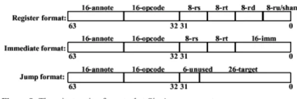
The SimAsync architecture is derived from the SimpleScalar architecture. Their instruction set architectures are all based on MIPS-IV ISA and are a superset of MIPS with several notable differences and additions [1]. First, there are no architected delay slots. Secondly, loads and stores support two addressing modes for all data types in addition to those found in the MIPS architecture. These are indexed (register + register) and auto-increment/decrement. Third, there is a square-root instruction implements both single and double precision floating point square roots. Finally, the instruction encoding uses 64-bit extended encoding.
Three instruction formats are supported. They are register, immediate, and jump formats. (see Figur e 9)
Like traditional pipelines, instructions are fetched by fetch unit, decoded and dispatched in dispatch unit, evaluated in execute unit, and then retired in commit unit.
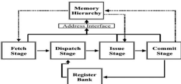
Figur e 10 describes the overview of
SimAsync architecture. It looks like the general structure of synchronous processor, but we know that the communications are using protocols instead of clocks. The details of each unit will be discussed in following sections.
4-2. Memor y Hier ar chy
The details of SimAsync memory hierarchy are described in Figur e 11[1]. The architecture of cache system and TLBs are adjustable. The characteristics can be adjusted by changing parameters just meets our expectancy.
4-3. Fetch Unit
The details of fetch stage are shown in
Figur e 12. The main job of the fetch unit is to
fetch instructions from instruction cache. The instruction address is determined by program count (PC, its initial value is determined by the loader). The fetch width is an architected parameter. It is determined by the product of the decode width of the dispatch stage and the speed of front-end of machine relative to execution core. The cycle time of the fetch unit is adjustable, too. If a cache miss is happened, no matter a pure cache miss or a TLB page fault, the fetch unit will end its job and stall until the miss solved.
In order to reduce the control penalty, we
need a branch predictor. If mis-prediction is happened, or any statistics are needed, the status of branch predictor will be updated in the commit stage. The default branch predict algorithm is to predict non-taken.
After the instructions are fetched, they are stored in the instruction fetch queue, which will be accessed by the dispatch unit afterward. Its size is also adjustable.
4-4. Dispatch Unit
Figur e 13 shows the details of the dispatch
stage. Before being executed, the instructions have to be decoded. The dispatch unit decodes the instructions, request register value from register bank and then saves the decoded instructions into buffer.
The decoder receives an instruction from instruction fetch queue, decodes the instruction and then requests the register values needed from register bank. Whenever input data dependency is solved or not, the decoded instruction will be send into the register update unit (RUU) with the information of data dependency. The decoder also records the output dependency of the instruction in a rename table.
The decode width is an architected parameter. The cycle time of the dispatch unit can be adjusted, too. Of course, the size of RUU and LSQ are also architected parameters.
The structure of each RUU element is described in Figur e 14. And the structure of each LSQ is show in Figur e 15.
The main function of the issue unit is to execute instructions. The details of the issue unit are shown in Figur e 16. The scheduler receives decoded instructions from RUU and LSQ, checks the data dependency is solved or not. If the data dependency is already solved, the scheduler put the instruction into the ready queue for the next step. If the in-order issue simulator is used, and the data dependency has not been solved, the issue stage will end its job and try to issue the hazard instruction next time. If the out-order issue simulator is used, the hazard instruction will be inserted back into the RUU / LSQ, and then the scheduler will check the next instruction continuously.
After scheduling, the issue unit gets those ready instructions from the ready queue. The issue unit request the functional unit needed by the instruction. The issue width, the number and latency of each functional unit type can be adjusted by the architected parameters. And keep in mind that the latency of floating point units is usually one hundred times of the latency of integer units.
4-6. Commit Unit
The final stage— the commit stage— is described in Figur e 17. First, the completed instructions are received from the event queue. The commit unit writes the result back to the register bank, including the value load from memory. If a branch mis-prediction is encountered, the commit unit will send the correct PC value to the fetch unit to fix the program flow, and then update the branch predictor status. The commit unit also refreshes the rename table to make certain data
dependency solved.
Store instruction is processing in this stage, too.
The stored value is sent to memory at this moment.
After that, the valid, completed
instructions will be committed. The commit unit will commit these changes in register bank and memory system. If there are invalid instructions (for example, wrong pre-fetch instructions), the commit unit retires these instructions directly without change the machine status. After the instructions are committed, the occupied RUU / LSQ element will be free.
The commit unit will also free the functional units which that complete their job. The commit width is another architected parameter.
The overall detailed architecture is shown in next page. Each stage is indicated by a dotted square with its name. Although the SimpleScalar architecture is not totally the same as our design, it reduces our develop effort very much and the differences can be accepted.
5. Implementation and Ver ification
Results
In this section, we will discuss the details of implementation of the simulators and provide some verification results.
5-1 Measur e the Execution Time
A simulator should be able to provide the information of execution time. We need to consider how to measure the execution time. In order to carry it out, we explain the measuring rules step by step.
As we mentioned before, the architecture simply divide in to four stages. They are Fetch, Dispatch, Issue, and Commit. Assume one cycle spends one nero-second (ns). We keep track of the timestamp of each stage and the initial values of them are all zero. We check every stage per event in reverse order to vanish the inter-stage synchronization. The reverse order can help us to reduce some design effort. If some stage finishes its work, its timestamp will be increased of its processing time.
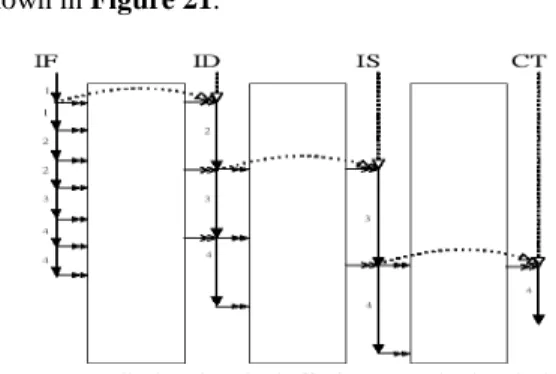
Figur e 19 describes the normal case. The
number inside each processing segment indicates the order of timestamp’s changes. Notice that we may change the timestamp more than once per check. It is nature that each stage should act as many times as it could. We can reduce the inaccuracy through this way. The white arrow indicates a delay is happened and we explain it in the next section.
Sometimes the timestamps can be increased normally, because in nature the stages have to stall until they can work. There are several cases that the timestamp have to be stalled.
Figur e 20 shows the first case. Assume
there is a stage with prior and successive queues, which used to be a buffer. When the prior queue is empty, no matter what status the successive queue is, the current stage has nothing to do. Thus the current stage will stall and must wait until the prior stage produces some new inputs into the prior queue. With the new inputs, the current stage has new job to do. In this case, the timestamp of the current stage will be set as the timestamp after the prior stage produces results. Recall Figur e 19, we see that the queues are all empty initially and the timestamps of back-end stages are set as the time that the prior stage completes its work. The timestamps setting is
shown in Figur e 21.
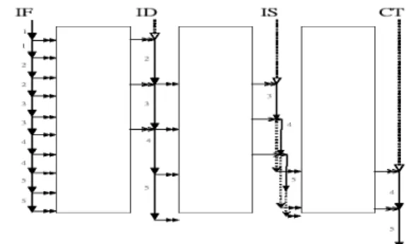
Another case is described in Figur e 22. When the successive queue of the current stage is full, no matter what status the prior queue is, the current stage will stall. Because there is no empty slot for new output to insert. The current stage will stall until there is an empty space in the successive queue, that means the next stage consume the data in the successive queue. In this case, the current stage must wait until the next stage done its job and keeps on work afterwards. In this case, the timestamp of the current stage will be set as the timestamp after the successive stage consume something from queue.
See Figur e 23, the dotted white double arrow shows that the fetch stage is stall at the third check. And when the fourth, the dispatch stage produces empty slots in the buffer and then set the timestamp of the fetch stage. Afterwards, the fetch stage can continue its job.
There are still other cases that the
timestamp has to stall. The usual processing time of the fetch stage is determined by the hit time of the level one cache, but it has to stall when a cache miss is happened. The fetch stage will stall until the cache miss recover. This case is
happened in the issue stage and the commit stage, too.
When a mis-prediction branch is
committed, there is something to do. As Figur e
24 describes, we have to reset the timestamp of
the fetch stage to the end of the commit stage. It indicates that the new PC changes the program flow and the fetch stage begins to fetch the correct instructions. The dotted white double arrow in Figur e 24 describes the correction we do.
We have developed several major rules about measuring the execution time. Besides, there are still some details need attention. Firstly, we recall that the processing time of each stage can be adjusted by configuration. In our simulation, the processing time of the dispatch stage is fixed. But others are varied with the situations the stages meet. In the fetch stage, as we mentioned, the processing time equals to the level one cache hit time usually. But sometimes, when a cache miss or a page fault is happened, it will be equal to the cache miss time or the TLB miss time. In the issue stage, if there are still empty function units, the processing time will be the processing time of the issue stage. Figur e 25 describes this situation. The processing time of the issue stage is a composite of the issue time and the functional unit latency. The issue time is indicated by a straight line and the functional unit is indicated by a dotted line. We can issue next instruction after the issue time passes. However, when there is no free function unit for the next instruction, the processing time will be the earliest finish time the specific type of function units. In the commit stage, because it processes the store instruction, it needs to consider the miss recovering time, too. When no miss is happened, the processing time of the commit stage will be the time the commit processing needs.
We also keep the timestamp within each individual instruction. This timestamp is used as double check. We can sure that each stage only processes an instruction when it is ready. See the commit stage in Figur e 25, the commit stage commit executed instructions only when they are ready at that time.
Since we can set all the architected parameter of processing time, we can get more precise simulation results through set the more practical parameters. According to consider each timestamp carefully, we can get the reasonable results.
5-2. Count the Data Dependency
In order to study how serious the data dependency will be. We also keep track of the number of dependency. As we mentioned before, there is a scoreboard to keep the status of the register bank. It records which instruction will attempt to modify the specific register. Before the issue unit issues an instruction, it checks the scoreboard first. If all source registers of the current instruction are ready, there is no data dependency. But if some of the sources are recorded as “lock”, it means that some previous instruction needs to modified it do not complete its job. In this case, the number of locked instruction will be increased. If the simulator is in in-order issue mode, the current instruction cannot be issued until the data dependency is solved.
5-3. Benchmar k
Table 1 is the list of the benchmarks we
used in our paper. And Table 2 is the characteristic of these benchmarks.
5-4. Simulator Settings
Before running the benchmarks, we have to decide all architected parameters. We set our simulator into three modes, they are in-order issue, out-of-order issue, and multiple function units (MFU). As the simulator is in in-order issue mode, it cannot issue the next instruction when the current instruction suffers from data dependency. We can get information about how serious the data dependency is through the in-order issue mode. In the out-of-order issue mode, the next instruction can be issued whether the current instruction is ‘locked’ or not. Of course, the instructions are committed in order. We ‘hide’ the delay of data dependency with the out-of-order issue mechanism. We hope to consider if it is worth to solve the problem with the mechanism. Usually, to use multiple function units is the popular way to improve the
performance of the processors. We simply increase the number of function units of the issue stage to see if the MFU can improve the performance of the asynchronous processors.
We will list the different architected parameters of the three modes (Table 3) and following is the common parameters (Table 4).
Notice that we use the uniform level 2 cache.
5-5. Ver ification Results
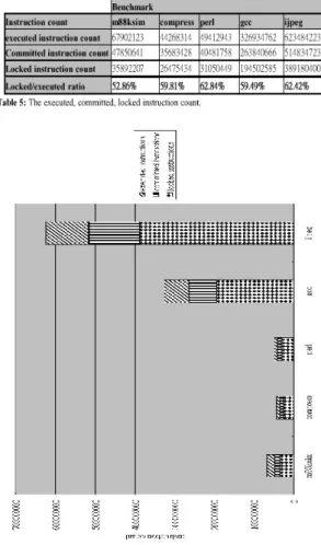
As we mentioned before, we run the benchmarks in the in-order issue mode to study the problem of data dependency. We count not only the ‘locked’ instructions but also the executed and committed ones. An instruction is executed when the issue unit issues it. But it does not mean that the execution is correct. Whenever a branch mis-prediction or an unconditional jump or an interrupt is happened, the pre-executed instruction will be retired directly. Only when an instruction is committed, the execution is correct. An instruction is called “committed” when it is committed by the commit unit. That’s why the execution instruction count is always larger than the committed instruction count.
Before an instruction is executed, it must be dispatched. Thus the delay of data
dependency influences the performance in early stage of the pipeline. In Table 5 we can see the ratio of the locked instruction count to the executed instruction count, too. They all range from 50% to 65%, and that is really a high ratio. We can realize that the data dependency does impact the performance very much and we should try to solve the serious problem in reasonable algorithms.
We also notice that the committed instruction count is the same as the count in the original synchronous processor simulator. That means our simulator is correct logically, and we still have to verify correctness of the simulation time.
Table 5 is the statistics of the three kinds
of instruction count of the benchmarks. And
Figur e 26 is the graphic description of this
statistics.
Table 6 is the statistics of the simulation
results of the benchmarks. We run the programs in three modes. The results are simulation time (in ns). The simulation time is calculated by keeping track of timestamp of each stage and follows the rules we have discussed in previous section.
We notice that the trend of the execution time of the three modes meets our expectancy. We also ran the same benchmarks by setting all parameters double. We got the simulation results almost double as original ones. Since we have verified the measuring rules with some small cases and we have the correct trend, we can say that the simulation result is very close to correct. We can realize some important facts from the results, too. Firstly, if an asynchronous processor is out-of-order issued, the delay of
data dependency is hidden and the performance is better than an in-order issued one. The difference of simulation time of the in-order issue mode and out-of-order issue mode can be treated as the delay of data dependency. We should still try to study a suitable algorithm, like data forward, to eliminate the delay indeed. Second, MFU indeed improve the performance, even our simulator is asynchronous. But the main improvement is come from the out-of-issue. Third, the running time can be just a reference, because the critical time of each unit is not drawn from the real world. We certainly can get a more believable result through setting the architected parameters based on simulation results of the EDA tools.
Table 6 is the running results and the
improvement ratio of each mode. Figur e 27 describes the running results.
The two running results can be used to prove that the asynchronous processor simulator is work. Since we have verified the correctness of the logicality and the time simulation is near to be correct, the reliability of the simulator is good enough.
In this paper, we design and implement a wanted simulator of asynchronous processors. Because the efforts of implementation, we design this simulator based on SimpleScalar and carefully think about how to maintain the timestamps of each stage. We also count the number of data dependency and can be helpful to the researches of solve the data hazard. This free tool set can be used to investigate the problems of the asynchronous architecture.
With this simulator, we can study some questions about the asynchronous architecture. To improve the performance, we should solve the difficulty of data forwarding. We also can study the arbitration of core processor and off-chip memory. The high power efficiency is the advantage of asynchronous design. We can trace the power usage and design the architecture using less power.
To be a complete simulator, SimAsync still has many things to do. For example, the execution time of ALU should be data dependent. We can make the design of the simulator to be more modular, such that the variable execution time can be simulated in our simulator. And then we can supports micronets after well defining the instruction types and microagents they will need.
References
[1] D. Burger et al. “The SimpleScalar Tool Set, Version 2.0”, University of
Wisconsin-Madison Computer Sciences Department Technical Report #1342, Jun, 1997
[2] T. Werner, V. Akella. “Asynchronous processor survey”, IEEE Computer Vol 30, Issue 11, Page(s):67-76, Nov. 1997 [3] Sutherland, I.E. “Micropipelines”,
Communications of the ACM, Vol.32, No.6, Page(s)720-738, Jun 1989
[4] D. K. Arvind et al. “Micronets: A Model for Decentralising Control in
Asynchronous Processor Architectures”, Asynchronous Design Methodologies, Proceedings, Second Working Conference, Page(s): 190 –199, 1995 [5] Furber, S.B.; Day, P.; Garside, J.D.;
Paver, N.C.; Woods, J.V. “AMULET1: a micropipelined ARM”, Compcon Spring '94, Digest of Papers, Page(s): 476 –485, 1994
[6] Woods, J.V.; Day, P.; Furber, S.B.; Garside, J.D.; Paver, N.C.; Temple, S. “AMULET1: an asynchronous ARM microprocessor”, Computers, IEEE Transactions on, Vol. 46 Issue 4, Page(s): 385 –398, April 1997
[7] Furber, S.B.; Garside, J.D.; Riocreux, P.; Temple, S.; Day, P.; Jianwei Liu; Paver,
N.C. “AMULET2e: an asynchronous embedded controller”, Proceedings of the IEEE, Vol. 87, Issue 2, Page(s): 243 –256, Feb. 1999
[8] Furber, S.B.; Garside, J.D.; Gilbert, D.A. “AMULET3: a high-performance self-timed ARM microprocessor”, ICCD '98. Proceedings. International
Conference on, Computer Design: VLSI in Computers and Processors. Page(s): 247 –252, 1998
[9] Lloyd, D.W.; Garside, J.D.; Gilbert, D.A. “Memory faults in asynchronous
microprocessors”, Fifth International Symposium on, Advanced Research in Asynchronous Circuits and Systems. Page(s): 71 -80, 1999
[10] Gilbert, D.A.; Garside, J.D. “A result forwarding mechanism for asynchronous pipelined systems”, Third International Symposium on, , Advanced Research in Asynchronous Circuits and Systems, Page(s): 2 –11, 1997
[11] Arvind, D.K.; Rebello, V.E.F. “On the performance evaluation of asynchronous processor architectures”, MASCOTS '95., Proceedings of the Third International Workshop on, Modeling, Analysis, and Simulation of Computer and
Telecommunication Systems, Page(s): 100 –104, 1995
[12] Donaldson, V.; Ferrante, J. “Determining asynchronous acyclic pipeline execution times”, Proceedings of IPPS '96, The 10th International, Parallel Processing Symposium, Page(s): 568 –572, 1996 [13] Arvind, D.K.; Rebello, V.E.F. “Static
scheduling of instructions on micronet-based asynchronous processors”, Second International Symposium on, Advanced Research in Asynchronous Circuits and Systems, Page(s): 80 –91, 1996
[14] Moore, S.W.; Robinson, P. “Rapid prototyping of self-timed circuits”, ICCD '98. Proceedings. International Conference on, Computer Design: VLSI in Computers and Processors, Page(s): 360 –365, 1998
[15] Lewis, M.; Garside, J.; Brackenbury, L. “Re-configurable latch controllers for low power asynchronous circuits”, Fifth International Symposium on, Advanced Research in Asynchronous Circuits and Systems, Page(s): 27 –35, 1999 [16] Riocreux, P.A.; Lewis, M.J.G.;
Brackenbury, L.E.M. “Power reduction in self-timed circuits using early-open latch controllers”, Electronics Letters, Vol. 36, Issue 2, Page(s): 115 –116, 20 Jan. 2000