適用於時變正交分頻多工系統之干擾消除技術

國 立 交 通 大 學

電信工程學系碩士班

碩士論文

適用於時變正交分頻多工系統之干擾消除技術

Interference Cancellation in OFDM Systems over

Time-Varying Channels

研 究 生：蔡宗翰 Student:

Tsung-Han Tsai

指導教授：李大嵩 博士 Advisor:

Dr.

Ta-Sung

Lee

適用於時變正交分頻多工系統之干擾消除技術

Interference Cancellation in OFDM Systems over

Time-Varying Channels

研 究 生：蔡宗翰 Student:

Tsung-Han Tsai

指導教授：李大嵩 博士 Advisor:

Dr. Ta-Sung Lee

國立交通大學

電信工程學系碩士班

碩士論文

A Thesis

Submitted to Institute of Communication Engineering

College of Electrical Engineering and Computer Science

National Chiao Tung University

in Partial Fulfillment of the Requirements

for the Degree of

Master of Science

in

Communication Engineering

June 2006

Hsinchu, Taiwan, Republic of China

適用於時變正交分頻多工系統之干擾消除技術

學生：蔡宗翰

指導教授：李大嵩 博士

國立交通大學電信工程學系碩士班

摘要

正 交 分 頻 多 工 系 統 為 新 一 代 無 線 通 訊 系 統 最 常 使 用 的 技 術 ， 如 IEEE 802.11a/g/n、 IEEE 802.16、IEEE 802.20、數位電視、數位廣播等許多系統均採 用此技術。傳統的正交分頻多工系統並不適用在高速移動的環境中，然而移動傳 輸是未來無線通訊系統的趨勢之一，如 IEEE 802.16e 可支援到車速 120 km/hour， 而 IEEE 802.20 更可支援到車速 250 km/hour。傳統的正交分頻多工系統可以有效 率地使用在非時變通道中，且僅需簡單的等化器，即可修正通道效應，但在移動 的環境中，通道隨著時間改變，使得接收端的子載波失去正交性，因而導致子載 波之間的相互干擾，使得解調變後的效能降低。雖然最小均方差等化器可以改善 此種干擾問題，然而其複雜度過高，不利於正交分頻多工系統採用。在本論文中， 吾人利用移動傳輸通道的特性對共軛梯度法做最佳事先處理，來降低最小均方差 等化器所需反矩陣運算的複雜度，使得接收端得以有效消去子載波間的干擾，而 能在移動的環境下運作。吾人藉由電腦模擬驗證此一新等化器在移動的環境中， 可有效改善位元錯誤率。

Interference Cancellation in OFDM Systems over

Time-Varying Channels

Student:

Tsung-Han

Tsai

Advisor:

Dr.

Ta-Sung

Lee

Institute of Communication Engineering

National Chiao Tung University

Abstract

Orthogonal Frequency Division Multiplexing (OFDM) is a popular technique in modern wireless communications. There are many systems adopting the OFDM technique, such as IEEE 802.11 a/g/n, IEEE 802.16, IEEE 802.20, Digital Video Broadcasting, Digital Audio Broadcasting, etc. On the other hand, mobile transmission is a trend in future wireless communications. For example, IEEE 802.16e supports vehicle speed up to 120 km/hour, and IEEE 802.20 supports vehicle speed up to 250 km/hour. OFDM systems can be used efficiently in time invariant environments with one-tap equalizers. However, subcarriers are no longer orthogonal to each other in time-varying channels, and this causes the intercarrier interference (ICI) and degrades the system performance. Although the minimum mean square error (MMSE) equalizer can be employed to solve this problem, it requires a high complexity and is impractical for an OFDM receiver to be implemented. To alleviate this problem, we propose a conjugate gradient based method with optimal precondition by employing the property of the mobile channel, which can reduce the complexity of the matrix inversion problem in the MMSE equalizer. Finally, we evaluate the performance of the proposed system and confirm that it achieves good BER performance in mobile environments.

Acknowledgement

I would like to express my deepest gratitude to my advisor, Dr. Ta-Sung Lee, for his enthusiastic guidance and great patience. I learn a lot from his positive attitude in many areas. Heartfelt thanks are also offered to all members in the Communication System Design and Signal Processing (CSDSP) Lab for their constant encouragement. Finally, I would like to show my sincere thanks to my parents for their invaluable love.

Contents

Chinese Abstract

I

English Abstract

II

Acknowledgement III

Contents IV

List of Figures

VII

List of Tables

XI

Acronym Glossary

XII

Notations

XIV

Chapter 1 Introduction

1

Chapter 2 Overview of Orthogonal Frequency Division

Multiplexing (OFDM) Systems

4

2.1 Orthogonal Frequency Division Modulation Systems... 4 2.2 Challenges to Orthogonal Frequency Division Modulation Systems in Mobile

Environments ... 11 2.2.1 OFDM System Model over Time-Varying Channels... 12

2.2.2 Intercarrier Interference in OFDM System due to Time-Varying

Channels... 14

2.3 Existing Techniques for OFDM Systems over Time-Varying Channels ... 16

2.3.1 Intercarrier Interference Self-Cancellation Scheme ... 16

2.3.2 Frequency Domain Equalizer Scheme... 21

2.4 Summary ... 22

Chapter 3 Introduction to Conjugate Gradient (CG) Algorithm 23

3.1.1 General Projection ... 24

3.1.2 Property of the Projection Method... 25

3.2. Overview of Krylov Subspace ... 26

3.3 Krylov Subspace Methods ... 28

3.3.1 Arnoldi’s Algorithm ... 28

3.3.2 Krylov Subspace Methods based on Arnoldi’s Algorithm... 30

3.3.3 Symmetric Lanczos Algorithm... 34

3.3.4 Conjugate Gradient Method... 35

3.5 Summary ... 37

Chapter 4 Proposed Low-Complexity Frequency Domain

Equalizer 38

4.2 Existing Low-Complexity Frequency Domain Equalizers ... 40

4.3 Proposed Preconditioned Conjugate Gradient (PCG) MMSE Equalizer ... 44

4.3.2 PCG LMMSE Equalizer ... 47

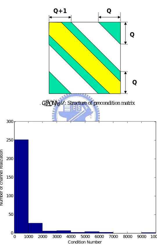
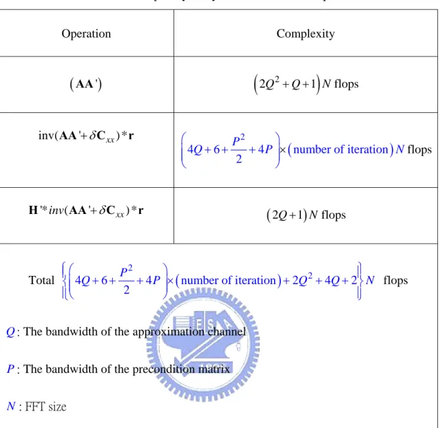
4.3.3 Optimum Precondition Matrix... 50

4.4 Complexity Analysis... 51

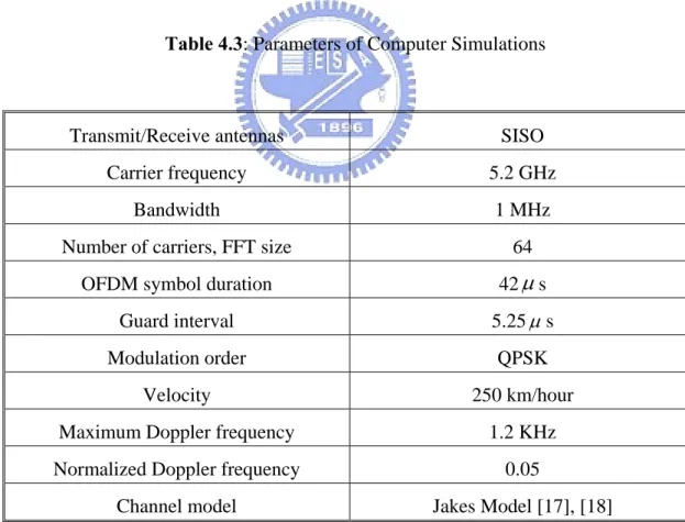
4.5 Computer Simulations ... 53

4.7 Summary ... 64

Chapter 5 Conclusion ... 65

List of Figures

Figure 2.1: OFDM signal with cyclic prefix extension... 7

Figure 2.2: A digital implementation of appending cyclic prefix into the OFDM signal in the transmitter... 7

Figure 2.3: Black diagrams of the OFDM transceiver. ... 10

Figure 2.4: ICI variance versus c (c is the index of super- or sub- diagonal) ... 15

Figure 2.5: Transmitter architecture of ICI self-cancellation... 17

Figure 2.6: Receiver architecture of ICI self-cancellation ... 18

Figure 2.7: ICI cofficients of different subcarriers ... 20

Figure 2.8: OFDM receiver architecture with frequency domain equalizer ... 22

Figure 4.1: Amplitude of frequency domain channel matrix in Jakes model ... 39

Figure 4.2: Structure of approximate frequency domain channel ... 40

Figure 4.3: MMSE equalizer (proposed by Xiaodong Cai and Georgios B. Giannakis)... 42

Figure 4.4: Partial MMSE equalizer (proposed by Philip Schniter) ... 43

Figure 4.5: Structure of precondition matrix... 49

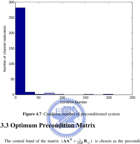
Figure 4.6: Condition number of original system ... 50

Figure 4.7: Condition number of preconditioned system... 50

Figure 4.9: BER performance obtained by using CG based MMSE equalizer. The performance of different numbers of iterations is shown. It can be seen

that it requires about 30 iterations to converge... 56

Figure 4.10: BER performance obtained by using PCG based MMSE equalizer, (BW of precondition matrix in PCG MMSE is zero). The performance of different numbers of iterations is shown. It can be seen that it requires about 4 iterations to converge. ... 57

Figure 4.11: BER performance obtained by using PCG based MMSE equalizer, (BW of precondition matrix in PCG MMSE is one). The performance of different numbers of iterations is shown. It can be seen that it requires about 3 iterations to converge. ... 58

Figure 4.12: BER performance obtained by using PCG based MMSE equalizer, (BW of precondition matrix in PCG MMSE is one). The performance of different numbers of iterations is shown. It can be seen that it requires about 2 iterations to converge. ... 59

Figure 4.13: BER performance of different schemes... 61

Figure 4.14: BER performance under different vehicle speeds. ... 62

List of Tables

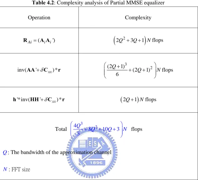
Table 4.1: Complexity analysis of PCG MMSE equalizer ... 52

Table 4.2: Complexity analysis of partial MMSE equalizer... 53

Table 4.3: Parameters of computer simulations... 54

Acronym Glossary

ADC analog-to-digital conversion

CP cyclic prefix

CG Conjugate gradient

DFT discrete Fourier transform

DIOM direct incomplete orthogonalization method FFT Fast Fourier Transform

FIR finite impulse response FSK frequency shift keying

ICI intercarrier interference IOM incomplete orthogonal method ISI intersymbol interference IFFT Inverse Fast Fourier Transform

LS least square

LANs local-area networks MCM multicarrier modulation MMSE minimum mean-square error NLOS non-LOS

OFDM orthogonal frequency division multiplexing PAPR peak-to-average power ratio

PCG preconditioned conjugate gradient

PHY Physical Layer

PSD power spectral density QPSK quadrature phase shift keying

RF radio frequency

SIR signal-to-interference ratio SNR signal-to-noise ratio

Notations

F DFT matrix

h time domain channel tap

H time domain channel matrix

A frequency domain channel matrix

c

N number of subcarriers

cp

N number of guard interval samples

DT

N number of data tones M modulation order

η AWGN noise

s transmitted frequency domain signal x transmitted time domain signal y received signal after DFT

R information data rate L channel order s T symbol duration W equalizer weights 2 n σ noise power

Chapter 1

Introduction

Orthogonal Frequency Division Multiplexing (OFDM) is a popular technique in modern wireless communication systems. There are many systems adopting this technique, such as IEEE 802.11 a/g/n, IEEE 802.16, IEEE802.20, Digital Video Broadcasting, Digital Audio Broadcasting, etc. In an OFDM system, the bandwidth is divided into several orthogonal subchannels for transmission. A cyclic prefix (CP) is inserted before each symbol. Therefore, if the delay spread of the channel is shorter than the length of the cyclic prefix, the intercarrier symbol interference (ISI) can be eliminated due to the cyclic prefix. On the other hand, subcarriers in OFDM are orthogonal to each other over time-invariant channels, so the conventional OFDM system only requires one-tap equalizers to compensate the channel response. This characteristic simplifies the design of the OFDM receiver, for this reason, the OFDM technique is widely used in wireless communication systems.

The mobile transmission is a trend in future wireless communications. Many systems support the mobile transmission, such as IEEE 802.16e, IEEE 802.20, DVB-H. and these systems also adopt the OFDM technique. However, while OFDM system is applied in mobile environments, the variation of channels destroys the orthogonality among subcarriers and therefore the intercarrier interference (ICI) arises. The conventional one-tap equalizer is insufficient for the mobile OFDM system because

the ICI degrades the system performance; the ICI cancellation technique plays an important role in mobile OFDM systems.

Many methods for ICI cancellation have been proposed. By mapping the data into groups of subcarriers, intercarrier interference self-cancellation scheme [1], [2] has been proposed. This scheme can reduce the computation complexity while sacrificing the transmission bandwidth efficiency. An error bound of the mobile OFDM system and an MMSE-SIC (minimum mean square error-successive interference cancellation) equalizer for canceling ICI are proposed [3]. Alternatively, an MMSE-PIC (parallel interference cancellation) equalizer is proposed in [4]. However, the computation complexity of these schemes is proportional to the square of the FFT size. On the other hand, some low complexity equalizers whose computation complexity increases linearly with the FFT size have been proposed in [5], [6], [7]. Those equalizers are based on approximations of the mobile channels. The ICI cancellation scheme in [5] can only be used in slow time-varying channel because of the rough approximation. An MMSE equalizer with a modified channel approximation and time-domain windowing technique for enhancing this approximation are introduced [6]. Another simple MMSE equalizer with the same channel approximation in [6] has been proposed [7] based on the LDLH factorization.

This paper proposes a low-complexity MMSE equalizer based on the band channel approximation in [6] and a conjugate gradient based method with optimal preconditioning by employing the property of the mobile channel, which can reduce the complexity of the matrix inversion problem in the MMSE equalizer. The preconditioned conjugate gradient (PCG) algorithm is one of the best known Krylov subspace method for solving spare, positive definite systems of equations which is equivalent to the matrix inversion problem in the MMSE equalizer. Many kinds of

Krylov subspace methods are introduced in [8], [9], [10]. The iterative programs for simulations in this thesis are based on the template book [11].

This thesis is organized as follows. In Chapter 2, the general idea of the OFDM system and the challenges it is faced with mobile environments are described. In Chapter 3, the basic idea of the Krylov subspace methods and the conjugate gradient (CG) methods are introduced. In Chapter 4, the proposed interference cancellation scheme is presented and analyzed. We evaluate the performance of the proposed system and confirm that it achieves good BER performance in mobile environments. In Chapter 5, we conclude this thesis and propose some potential future works.

Chapter 2

Overview of Orthogonal Frequency

Division Multiplexing (OFDM)

Systems

In this chapter, an overview of OFDM systems will be given in Section 2.1. OFDM is an efficient technique for high data rate transmission such as IEEE 802.11 a/g/n, IEEE 802.16. We will show the advantage of OFDM system and why traditional OFDM system can be efficient in frequency-selective environments. Furthermore, the challenge of OFDM system in mobile environments is presented in Section 2.2 and some existing techniques for mobile OFDM system is introduced in Section 2.3

2.1 Orthogonal Frequency Division Modulation

Systems

OFDM is a special case of multicarrier transmission, where a single data stream is transmitted over a number of low data rate subcarriers. OFDM can be thought of as a hybrid of multicarrier modulation (MCM) and frequency shift keying (FSK) modulation scheme. The principle of MCM is to transmit data by dividing the data stream into several parallel data streams and modulate each of these data streams onto

individual subcarriers. FSK modulation is a technique whereby data is transmitted on one subcarrier from a set of orthogonal subcarriers in symbol duration. Orthogonality between these subcarriers is achieved by separating these subcarriers by an integer multiples of the inverse of symbol duration of the parallel data streams. With the OFDM technique used, all orthogonal subcarriers are transmitted simultaneously. In other words, the entire allocated channel is occupied through the aggregated sum of the narrow orthogonal subbands.

The main reason to use OFDM systems is to increase the robustness against frequency-selective fading or narrowband interference. In a single carrier system, a single fade or interference can cause the entire link fail, but in a multicarrier system, only a small amount of subcarriers will be affected. Then the error correction coding techniques can be used to correct errors. The equivalent complex baseband OFDM signal can be expressed as

1 2 ₁ 2 2 2 ( ) 0 ( ) ( ) ( ) 0 Otherwise c c c c N N k k N k k T k _N k d t t T x t φ φ − − =− =− ⎧ ⎡ ⎤ ⎪ _{≤ ≤} ⎢ ⎥ ⎪ =_⎨ =_{⎢ ⎥} ⎪ _{⎢ ⎥} ⎣ ⎦ ⎪⎩

∑

_∑

where Nc is the number of subcarriers, T is the symbol duration, dk is the transmitted

subsymbol (M-PSK or M-QAM), ( ) j2 f tk /

k t e T

π

φ = is the kth subcarrier with the frequency /f_k =k T , and uT(t) is the time windowing function. Using the

correlator-based OFDM demodulator, the output of the jth branch can be presented as

1 2 2 * 0 2 1 ( ) ( ) c c N k j 0 j t T T _T j j k N k j y x t t dt d e dt T d π φ − − =− = = =

∑

∫

∫

By sampling x(t) with the sampling period Td=T/Nc, the discrete time signal xn can be expressed as 1 ₂ 2 2 1 , 0 1 ( ) IFFT{ } 0 , Otherwise c c c d N k j n N k c N n t nT c _k k d e n N x x t N d π − = ₌₋ ⎧ ⎪ ≤ ≤ − ⎪ = =_⎨ = ⎪ ⎪⎩

∑

Note that x is the Inverse Fast Fourier Transform (IFFT) output of the N input data _n subsymbols. Similarly, the output of the j-th branch can also be presented in the digital form 1 2 1 ₂ 0 2 1 FFT{ } [ ] c c c c N j j n N N j n k k N n c _k y x x e x k j d N π δ − − − = ₌₋ = =

_∑

_∑

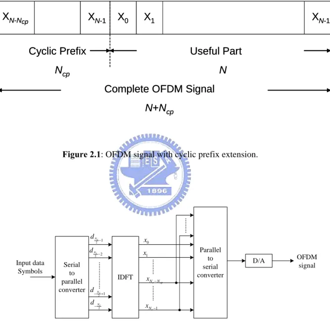
In theory, the orthogonality of subcarriers in OFDM systems can be maintained and individual subcarriers can be completely separated by the Fast Fourier Transform (FFT) at the receiver when there are no intersymbol interference (ISI) and intercarrier interference (ICI) introduced by transmission channel distortions. However, it is impossible to obtain these conditions in practice. In order to eliminate ISI completely, a guard interval is imposed into each OFDM symbol. The guard interval is chosen larger than the expected delay spread, such that the multipath from one symbol cannot interfere with the next symbol. The guard interval can consist of no signals at all. However, the effect of ICI would arise in that case due to the loss of orthogonality between subcarriers. To eliminate ICI, the OFDM symbol is cyclically extended in the guard interval to introduce cyclic prefix (CP) as shown in Figures 2.1 and 2.2. This ensures that delayed replicas of the OFDM symbol always have an integer number of cycles within the FFT interval, as long as the delay is smaller than the guard interval.

X

X

X

X

X

Cyclic Prefix

N

Useful Part

N

Complete OFDM Signal

N+N

X

X

X

X

X

Cyclic Prefix

N

Useful Part

N

Complete OFDM Signal

N+N

Figure 2.1: OFDM signal with cyclic prefix extension.

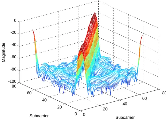
Serial to parallel converter Input data Symbols IDFT 2 1 Nc d ₋ 2 2 Nc d ₋ 2 Nc d₋ 2 1 Nc d_{− +} .... .... ... .... . 0 x 1 x 1 c N x .... .... . c cp N N x − .... .... . .... .... . − Parallel to serial converter OFDM signal D/A

Figure2.2: A digital implementation of appending cyclic prefix into the OFDM signal

As a result, the delayed multipath signals which are smaller than the guard interval will not cause ICI. The complete OFDM signal with CP is given by

1 _{2 ( )} 2 2 1 0 1 0 Otherwise c cp c c N k j n N N k c N n _{c k} d e n N N x N π − ₋ =− ⎧ ⎪ cp ≤ ≤ + − ⎪ = ⎨ ⎪ ⎪⎩

∑

where Ncp is the number of samples in CP. Due to CP, the transmitted OFDM symbol

becomes periodic, and the linear convolution process of the transmitted OFDM symbols with the channel impulse responses will become a circular convolution one. Assuming the value of Ncp is larger than the channel length, the received signal vector

can be expressed as = + y Hx η (2.6) 0 1 0 1 0 0 1 0 0 1 1 1 1 0 0 0 0 0 0 0 0 0 c cp cp c c cp cp N N N N N N N h x h h h y x h h x h h y x h η η − − − − − ⎡ ⎤ ⎢ ⎥ ⎡ ⎤ ⎢ ⎥ ⎢ ⎥ ⎢ ⎥ ⎢ ⎥ ⎡ ⎤ _{⎢ ⎥ ⎢ ⎥} ⎡ ⎢ ⎥ _{⎢ ⎥ ⎢ ⎥} ⎢ = ⎢ ⎥ _{⎢ ⎥ ⎢ ⎥} ⎢ ⎢ ⎥ _{⎢ ⎥ ⎢ ⎥} ⎢ ⎣ ⎦ ⎣ ⎢ ⎥ ⎢ ⎥ ⎢ ⎥ ⎢_⎣ ⎥_⎦ ⎢ ⎥ ⎣ ⎦ y η x H ⎤ ⎥ + _⎥ ⎥ ⎦

Applying SVD on the channel response, we have

(2.7)

H

=

H UΣV

where U and V are unitary matrices, and is a diagonal matrix. Substituting Equation (2.7) and the equalities of

Σ

V and UH

= =

x X Y y into Equation (2.6), the

(2.8) ( ) H H H H = = + = + = + U η Y U y U Hx η U HVX N ΣX N

This means that the output Y can be expressed in terms of the product of and X plus noise. When

Σ

i N i

x₋ =x ₋ for i=1,...,N_cp, a more compact matrix form of the guard interval can be written as

(2.9) 0 1 1 0 1 0 0 0 1 _{1 0} 1 1 0 0 0 0 0 0 0 0 0 0 cp cp cp c _cp c c cp cp N N N N _N N N N h h h h h h h y x h h y _{h h h} x h h h η η − − − ⎡ ⎤ ⎢ ⎥ ⎢ ⎥ ⎢ ⎥ ⎡ ⎤ _{⎢ ⎥}⎡ ⎤ ⎡ ⎢ ⎥ _{⎢ ⎥}⎢ ⎥ ⎢ = + ⎢ ⎥ _{⎢ ⎥}⎢ ⎥ ⎢ ⎢ ⎥ _{⎢ ⎥}⎢ ⎥ ⎢ ⎣ ⎦ _{⎢ ⎥}⎣ ⎦ ⎣ ⎢ ⎥ ⎢ ⎥ ⎢ ⎥ ⎣ ⎦ 0 1 N − ⎤ ⎥ ⎥ ⎥ ⎦

where H becomes a circulant matrix (H F ΛF ) and Q is a discrete Fourier = H transform (DFT) matrix with the lth entry as

2 1 c l j N l c e N π − = F (2.10)

As in Equation (2.8), the received signal y can be transformed into Y

(2.11) ( ) H H H H H = = + = + = + Σ _N Y F y F Hx η F HF X F η ΣX N

According to Equation (2.11), by adding CP to the OFDM symbol, the modulation in OFDM is equivalent to multiplying the frequency domain signals of the OFDM symbol with the channel’s frequency responseΣ.

The block diagrams of the OFDM transceiver is shown in Figure 2.3, where the upper path is the transmitter chain and lower path corresponds to the receiver chain. In the center, IFFT modulates a block of input values onto a number of subcarriers. In the

receiver, the subcarriers are demodulated by the FFT, which performs the reverse operation of the IFFT. In fact, the IFFT can be made using the FFT by conjugating input and output of the FFT and dividing the output by the FFT size. This makes it possible to use the same hardware for both transmitter and receiver. This complexity saving is only possible when the transceiver doesn’t have to transmit and receive simultaneously. The functions before the IFFT can be discussed as follows. Binary input data is first encoded by a forward error correction code. The encoded data is then interleaved and mapped onto QAM values. In the receiver path, after passing the radio frequency (RF) part and the analog-to-digital conversion (ADC), the digital signal processing starts with a training sequence to determine symbol timing and frequency offset. The FFT is used to demodulate all subcarriers. The FFT outputs are mapped onto binary values and decoded to produce binary output data. In order to successfully map the QAM values onto binary values, the reference phases and amplitudes of all subcarriers have to be acquired first.

Binary Input Data

Binary Output Data

Coding Interleaving QAM Mapping

Pilot Insertion

Serial to Parallel

Decoding _interleavingDe- _MappingQAM _CorrectionChannel Parallel to_Serial

IFFT (TX) FFT (RX) Parallel to Serial Serial to Parallel Add Cyclic Extension

and Windowing DAC

RF TX

Remove Cyclic Extension Timing and Frequency

Synchronization ADC

RF RX

In conclusion, OFDM is a powerful modulation technique that simplifies the removal of distortion due to the multipath channel and increases bandwidth efficiency. The key advantages of OFDM transmission scheme can be summarized as follows:

1. OFDM is an efficient way to deal with multipath. For a given delay spread, the implementation complexity is significantly lower than that of a single carrier system with an equalizer.

2. In relative slow time-varying channels, it is possible to significantly enhance the capacity by adapting the data rate per subcarrier according to the signal-to-noise ratio (SNR) of that particular subcarrier.

3. OFDM is robust against narrowband interference because such interference affects only a small amount of subcarriers.

4. OFDM makes single-frequency networks possible, which is especially attractive for broadcasting applications.

2.2 Challenges to Orthogonal Frequency Division

Modulation Systems in Mobile Environments

The most important issue of the OFDM technique in time varying channels is that the ICI degrades the system performance. In this section, we will first introduce the mobile OFDM system model, and then discuss why the ICI is produced.

2.2.1 OFDM System Model over Time-Varying

Channels

The OFDM system model over time-varying channels is considered here. Assuming that is the i-th “frequency-domain” symbols, the OFDM symbol can be converted to “time-domain” symbols by N-point IDFT operation as

( ) ( ) 0 [ , ] i i i N s s ₋ = s … ₁ T 2 1 ( ) ( ) 0 1 ( ) , -N j kn i i _N c k k x n s e N n N π − = =

_∑

where is the maximum delay spread of the channel, is the length of CP, and W

(2.12)

where x(n) is serially transmitted over noisy time-varying multipath channels, incorporates a cyclic prefix of length . The channel is modeled by the time-varying discrete impulse response, , which is defined as the response of time n to an impulse response applied at time n-l.

c

N

( , )

h n l

The received sample sequence which is the convolution between the transmitted symbol and the time-varying channels can be written as

(2.13) 1 ( ) ( ) ( ) ( ) 0 ( ) ( , ) , 0 v i i i i n l n l r n h n l x η n N − − = =

_∑

z are the samples of additive white Gaussian noise (A GN), with variance σ 2. r the ISI free case, the delay spread of the channel should be shorter than the length of CP, as follows v≤N .

Fo

Then the receiver computes an N-point DFT operation to obtain the frequ c ency-domain signal 2 1 ( ) ( ) 0 1 ( ) , -N j mn i i _N n c n y m r e N n N N π − = =

_∑

Let ( , ) 1 j(2 /N lk) , 0 , -1 N l k = e− π ≤l k N F ≤ ⎤ ⎥ ⎥ ⎥ ⎥⎦ 1 1 i + ⎥ ⎥ −

be the standard N-dimensional DFT matrix, Equation (2.12) can be written in matrix form

( ) ( ) ( ) ( ) ( ) ( ) ( ) ( ) 0 ( ) ( ) _{( ) ( )} 1 ( ) ( ) (0, 0) 0 (0, 1) (0,1) (1,1) (1, 0) 0 (2,1) 0 ( 2, 1) ( 1, 1) 0 0 0 ( , 1) ( 1, 0) 0 0 0 0 ( 1, 2) ( 1, 0) i i i i i i i i i i _{i i} N i i h h L h h h r h h L L h L L r _{h L L h N L} h N L h N − ⎡ ₋ ⎤ ⎢ ⎥ ⎢ ⎢ ⎡ ⎤ _{⎢ − −} ⎢ _{⎥ ⎢} = ⎢ ⎥ _⎢ − − ⎢ _{⎥ ⎢} ⎢ ⎥ − + − ⎣ _{⎦ ⎢} ⎢ ⎢ − − − ⎢⎣ ⎦ ( ) ( ) 0 0 ( ) ( ) 1 1 i i i i N N x x η η − − ⎥ ⎥ ⎡ ⎤ ⎡ ⎥ ⎢ ⎥ ⎢ ⎥_{⎢ ⎥ ⎢+} ⎥ ⎢ ⎥ ⎢ ⎥ ⎢_⎣ ⎥ ⎢_{⎦ ⎣} ⎥ ⎥ ⎥ ⎥ (2.15) ( ) ( , ) i

h n l represents the channel response of the l th tap at the time instance n, we can

rewrite the above equation in matrix form as

(2.16) ( ) (i) ( ) ( ) , 0 i i i n N = + ≤ < r H x η where , , and , H is

the time-varying channel matrix. Equation (2.16) can be rewritten as

( ) ( ) ( ) 0 1 [ i , , i ] i T N r r ₋ = r … ( ) ( ) ( ) 0 [ i , , i ] i T N η η ₋ = η … ( ) ( ) ( ) 0 [ i , , i ] i T N x x ₋ = x … (2.17) ( ) ( ) ( ) ( ) ( ) ( ) ( ) i i i i H i i = + = + r H x η H F s η

We define as the frequency domain channel matrix and Equation (2.14) can be rewritten in vector form as

( )i H = (i) A FH F (2.18) ( ) ( ) ( ) ( ) ( ) ( ) ( ) ( ) ( ) ( ) ( ) i i i i i i H i i i i i = = + = + = y Fr FH x Fη FH F s Fη A s z

where A(i) has the form

(2.19) ( ) (0, 0) (0, 1) ( 1, 0) ( 1, 1) i A A N A N A N N − ⎡ ⎤ ⎢ = ⎢ ⎢ − − ⎥ ⎣ ⎦ A

which is called “equivalent frequency domain channel”, and the non-diagonal terms of produce the ICI.

A

2.2.2 Intercarrier Interference in OFDM System due

to Time-Varying Channels

In time-invariant channels, the A matrix in Equation (2.19) will be a diagonal matrix, so the conventional OFDM systems can compensate the fading channel with one-tap equalizers. In time-varying channel, the A matrix is no longer a diagonal matrix, so it will have a poor performance if one-tap equalizers are used. It can be indicated that the non-diagonal terms in the A matrix are the ICI terms.

We analyze the ICI power based on the theorem in [5], [6]. Assuming a typical wide-sense stationary uncorrelated scattering (WSSUS) channel model [12] as below

*

{ ( , ) ( , )} _t( ) _l ( ) E h n l h n q l− −m =r q σ δ2 m

where r q_t( ) is the normalized tap autocorrelation, and σ_l2 is the variance of the lth tap.

Since the non-diagonal terms in the A matrix are the intercarrier interference terms, we will compute the power of these non-diagonal terms. Let A n l( , ) be the n-th row, l-th column term of A, and denotes the N-point rectangular window. Finally, we obtain ( ) u n

{

}

{

}

(

)

∑

_∑

_∑

2 2 1 ₂ ( ) ( ) ( ) exp( ) l t l p n j pc u m u n r q N N π σ ∞ ∞ ∞ =−∞ =−∞ =−∞ − =

_∑

_{∑ ∑}

where denotes the nth supper or upper-diagonal. Assuming Rayleigh fading as in [10], we obtain ( ,: h ± )n s 0 ( ) (2 ) t d r q =J π f T q 2 2 1 , 2 ( ) (2 ) 0 , otherwise d s d s f T S f T φ π φ π φ ⎧ _≤ ⎪ =⎨ − ⎪ ⎩ (2.21)

where J₀ denotes the first kind zeroth-order Bessel function, and f T is the _{d s} maximum Doppler shift normalized to OFDM symbol rate.

-150 -100 -50 0 50 100 150 -102 -101 -100 C IC I fdTs=0.05 fdTs=0.01

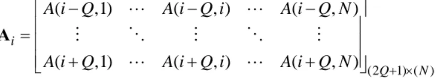
By Equations (2.20) and (2.21), we can simulate the power of the non-diagonal rms, which is the terms caused the ICI. Figure.2.4 shows the computer simulations ccording to Equations (2.20) and (2.21). We can observe that the coefficients of the equency domain channel matrix have most power on the central band and the edges f the channel matrix. One kind of channel approximation based on this property is escribed in Chapter 4. This channel approximation is the base of the low-complexity lgorithm which will be described later.

2.3 Existing Techniques for OFDM Systems over

ime-Varying Channels

OFDM is a strong candidate for high-data-rate systems over wireless channels. High data rates give rise to frequency-selective channels, while mobility and frequency error

2.3.1 Intercarrier Interference Self-Cancellation

ICI self-cancellation scheme is a simple way for suppressing ICI in OFDM system. It is to modulate one data symbol onto adjac te a fr o d a

T

s introduce time-selective channel. Due to the analysis in Section 2.2, we show that the traditional OFDM system is sensitive to time-varying channels. Some techniques have been proposed to mitigate the ICI. We will first introduce ICI self-cancellation scheme [1], [2], which is originally used in compensating frequency errors and also valid over time-varying channels. Then we will show the frequency domain equalizer technique for compensating the ICI.

Scheme

This method is proposed in [1], [2]. The

ent pairs of subcarriers rather than onto single subcarriers. By this way, the ICI generated by these adjacent subcarriers can be “self-cancelled” by each orther. This

scheme is also called polynomial cancellation (PCC). We will first analyze the ICI with single frequency as in [1],[2], and then show why the ICI self-cancellation works. The received signal on each subcarrier can be seen as a linear combination of signals received via different paths with different Doppler shifts. So that this scheme can also be used in the practical mobile environments that have significant Doppler spread.

The system architecture of the ICI self-cancellation scheme is shown in Figures 2.5-2.6. The only difference between the OFDM system with the ICI self-cancellation

e will show how this block works.

tion scheme

conventional scheme and the conventional OFDM system is the ICI self-canceling modulation/demodulation. W

Randomizer FEC Iinterleavr Modulation ICI Canceling

Modulation

IFFT Add DAC Filter RF DATA

CP

Figure2.6: Receiver architecture of ICI self-cancellation

Let the n-th OFDM transmission data be

2 1 2 1 0 ( ) c N j mn j f t _N m N m x n e s e π π − = =

_∑

e that the signal is mixed with a loca . In the

receiver, we ignore the noise terms and assum l

oscillator which has frequency mismatch Δ with the transmitter oscillator. Then the f demodulated signal in the receiver before FFT can be written as

2 1 (2 ) 1 0 ( ) N j mn j ft _N m N m r n e π θ s e − Δ + = = ×

_∑

optimum timing. After the samp

π

, and assuming this signal is sampled at the ling, the signal can be rewritten as

2 2 1 ( ) 0 1 ( ) n fT N j mn j j _{N N} k m r n e e s e N π π θ Δ − = = × ×

_∑

The sampled signal after DFT are given by

2 1 0 ( ) nd N j N n n y d r e π − − = =

_∑

By Equations (2.22) and (2.23), we have the received signals after sampling and DFT 2 2 2 1 1 0 0 ( ) nd n fT N N j ( ) 1 _j j mn j N N N m n m y d e e s e N π π π θ Δ − − = = = ×

_{∑ ∑}

_{∑ ∑}

The analysis of ICI terms can be done by defining complex weighting,

fT n m +Δ = = (2.24) N c₀ c_N−1,

which is the contribution of each input signal s₀ s_N−1.

N 0 ( ) j _{m d m} m 1 y d e θ c ₋ s = =

_∑

Compared Equations (2.24) with (2.25), we have the complex weighting written as

2 1 ( ) 0 1 N j n m d fT j _N m d n c e e N π θ − − +Δ − = = ×

_∑

(

)

By the aforementioned equation, we show the complex weighting value in Figure 2.7. The figure shows a smooth curve, this w

works.

th alled IC

the data ne onto adjacent subcarriers w h different

ill be the key point why ICI self-cancellation

Zhao and Haggman have proposed a me od to mitigate ICI c I self-cancellation scheme. This scheme maps to

it signs, such as s₀ = −s s₁, ₂ = −s₃,…,s_N−2= −s_N−1 . The difference between the adjacent coefficients is small, and the adjacent subcarriers map to the

be self-canceled by each other. The received signal after FFT can be written as

2 1 0 ( ) ( ) N j m m d m d m m even y d s e θ c c − − + − = ∈ =

_∑

_∑

In order to maximize the output SNR, the values y d , ( ) y d( + should be subtracted 1) in pairs as shown below

(y d)= y d( )−y d( + 1) ] j 2 1 1 1 0 N m m d m d m d m d m k m ( )[2 m s e θ c c c c c =

_∑

where ( )y d is the symbol that will be demodulated to obtain the information bits. By this way, the overall system SNR increases by a factor 2, due to the coherent addition.

Figure2.7:ICI cofficients of different subcarriers

0.8 -40 -30 -20 -10 0 10 20 30 40 -0.2 -0.1 0 0.1 0.2 0.3 0.4 0.5 0.6 Real 0.7 _Imaginary

A disadvantage of this system is that its bandwidth efficiency is only half of the conventional OFDM system. There are some new researches to improve the bandwidth

ancel the ICI produced by a frequency error due to mismatch between the transmitter nd receiver oscillators in the above description. In real mobile environments, the

ceived signal on each subcarrier can be seen as a linear combination of signals ceived via different paths with different Doppler shifts. So this scheme can also be sed in the practical mobile environments that have significant Doppler spread.

.3.2 Frequency Domain Equalizer Scheme

Frequency domain equalizer is a method which is used frequently in ompensating the ICI of OFDM systems in mobile environments. The transmitter rchitecture is the same as conventional OFDM system. Besides, a frequency domain

equalizer after FFT FDM systems in

the receiver before FFT are usually called the “Time Domain Signals”, and those after FFT are called the “Frequency Domain Signal”. By this definition, the frequency domain equalizer equalizes the received signal after FFT. There are many equalizers technique can be used here with different performance and complexity, such as block minimum mean square equalizer (MMSE) or block Zero-forcing (ZF), FIR equalizer, etc. The block of MMSE and ZF equalizer is shown below.

efficiency, such as in [13]. We only show that ICI self-cancellation scheme can self c a re re u

2

is added as shown in Figure 2.8. The signals of O

2 1 ( H ) H MMSE ₂ N s W H H ση I H σ − = + (2.29) 1 ( H ) H ZF W = H H − H (2.30)

where W is the equalizer weighting, H is the channel matrix in time domain, σ_η2 is the noise power, and σ_s2 is the signal power. Some low-complexity equalizers have already been proposed, as in [3], [4], [5], [6], [7]. This paper also proposed a low-complexity technique based on the block MMSE equalizer and will be shown in Chapter 4.

Figure2.8: OFDM receiver architecture with frequency domain equalizer

the OFDM system over time-varying channels. In particular, the ICI is e major subject of interest. We also introduce some existing techniques for solving this problem, such as the ICI self-cancellation schemes and the frequency domain equalizer schemes. Finally, modified OFDM systems for time-varying channel are presented.

2.4 Summary

In this chapter, we first introduce the traditional OFDM system, and show the challenges to th Derandomizer Decoding Bit interleaver Demodulation FFT Remove CP Filter DAC RF DATA Frequency Domain Equalizer

Chapter 3

Introduction to Conjugate Gradient

(CG) Algorithm

asic concept of projection and then introduce the Krylov subs

3.1 Projection Methods

We will first show the general projection theory [9], [10] and then show the projection can minimize error between the real solution and the approximate solution obtained by the projection methods.

We will first show the b

pace and some krylov subspace methods that are the predecessor of conjugate gradient methods. The evolution from basic Krylov method to conjugate gradient method is shown in Section 3.4. The Krylov subspace method is currently to be the most important iterative technique for solving large linear systems, and the CG algorithm is a mature algorithm in this topic.

3.1.1 General Projection

practical iterative techniques for solving linear systems . A projection method can be seen as a scheme of extracting approximate solution of a linear system from a subspace. We call this subspace the arch subspace or the candidate approximants denote by K. Assume that it has the he of these constraints is l independent conditions. e define a subspace L, which is called the subspace of constraints or left subspace. ere are two kinds of projection methods, orthogonal and oblique. An orthogonal proje

Most of the existing utilize a projection method an

se

dimension n. In general, there should have n constraints be imposed to be exacting t approximate solution. A typical way

W Th

ction means that the subspace L is the same as K. The oblique projection means that the subspace L is different from K, and they can have some relationships or be totally uncorrelated.

We show the mathematically approach of projection the technique. A projection technique onto the subspace can obtain approximated solutionˆx by

ˆ

Search x∈K and b−Axˆ⊥L (3.1)

or with initial guess x₀

0

ˆ

Search x∈x + and K b−Axˆ⊥L (3.2)

Defining the initial residual vector r₀ as r₀=b Ax- ₀, then Equation (4.2) can be written as 0 ˆ , x=x +σ σ∈K 0 (r -Aσ, )q = ∀ ∈0, q L (3.3)

Let P=[p₁,…p_n] be a basis of K, and Q=[ ,q₁…q_n] be a basis of L. Then the approximate solution in Equation (4.3) can be written as

0

ˆ

x=x +Py (3.4)

By b−Ax= −b Ax₀−AVy andQT(b−Ax)=0, we have

1 0

( T ) T

y= Q AP − Q r (3.5)

By Equations (4.4) and (4.5), we have the projection method based on Equation (4.2) in the matrix form, which is

1

0 0

ˆ ( T ) T

x=x +P Q AP − Q r (3.6)

3.1.2 Property of the Projection Method

We will show that orthogonal projection solution can minimize the error between the desired solution and the approximate solution as in [9]. Let P is the orthogonal projector onto a subspace K, x is the desired vector, and y is the arbitrary vector in subspace K. Because of the orthogonality betweenxandPx, we have

2 2 2 2 , x 2 2 2 2 y x Px y − = − − = Therefore, Px+ x−Px + Px−y y∈ (3.7) K 2 2 , y K x y x Px

∀ ∈ − ≥ − , we know that the orthogonal projection can m nimize 2-norm error between i x and y . Let y' is the orthogonal projection from

x onto subspace K, and then we have y′∈K

x− ⊥y′ K (3.8)

If A is a symmetric and positive definite matrix, we can derive the similar result that orthogonal projection can minimize A-norm error between x and y . By Equation (4.6)

( ( ), ) 0 , , we have

Ax=b,

By Equatio ′

− = ∀ ∈ (3.10)

T s is called the Galerki

n (4.7) can be rewritten as

K (b Ay q, ) 0 , q

hi n condition which defines an orthogonal projection [9]. Let A is an arbitrary matrix, and L= AK. The oblique projection onto K and orthogonal to L will minimize the 2-norm the residual vector . The derivation is similar as the orthogonal projection. Then we have

(3.11)

his is called the Petrov-Galerkin condition which defines an oblique projection [9].

3.2

The Krylov subspace is a subspace of the form [8],[9],[10]

(3.12)

By this definition, we know that is the subspace of all vectors in

of r= −b Axˆ

(b−Ay v′, )=0 , ∀ ∈v AK

T

. Overview of Krylov Subspace

2 -1 0 0 0 0 0 ( , ) span{ , , …, } m m K A r = r Ar A r A r m K n that can be x

written as = polynomial A( ) *r₀ and

fied system first. Then is an approximate so

should satisfy

n as a new linear system

the degree of polynomial do not exceed r₀. We will show the iterative methods are located in the Krylov subspace. Solving x = , we may solve the simplib

A Tx₀ =b x₀

lution for x . We may correct the approximation x with δ , so δ ₀

0

( )

A x +δ = (3.13) b

This can be see

(3.14)

0

We may solve Equation (3.13) by a simplified approximate system

(3.15)

rrect the approx

By settingT I the Equation

)

Multiplying Equation (3.16) by and adding , we have

(3.18) that 1 ( ) ( )i i i i r₊ = I −A r = I −A + r =p₊ 0 Tδ = −b Ax

Then the new approximate solution will be x₁ =x₀ +z₀. We may again co imate solution with the same process respect tox . Therefore, we have ₁

1 1_{( )} i i i i x x x T b Ax δ + − = + = + − (3.16) = , (3.13) can be written as 1 ( ) ( ) i i i i i i x ₊ =x + b−Ax = +b I −A x =x +r (3.17 A − b 1 i i i b−Ax + = −b Ax −Ar is the same as 0 ( )A r (3.19) 1 1 0

By r_i+1 ≤ I −A r_i , this result shows that we have guaranteed the convergence for any initial r₀ if I −A ≤1 Assuming that A has n eigenvectors with corresponding eigenvectors

i

a

j

λ , we write the initial residual r as ₀

i ia ξ =

_∑

al of the system depends on how well the polynomial p dam_i 0 1 n ( ) i i i i i p a ξ λ =

∑

Equation (3.18) shows that the residu ps the initial error.

By Equation (3.14), the i-th approximate solution x can be expressed as _i

i

x =x +r +

k =

(3.22)

The aforementioned discussion shows that iterative methods are located in the

space (see Section 3.1), different

projection methods can be obtained, such as orthogonal or oblique projection, and different kinds of iterative techniques have been derived. They have different

on a case by case basis. Usually, the characteristic of

iterative method. Choosing an appropriate method can have significant improvement ate and the complexity.

3.3 Krylov Subspace Methods

m kinds of K e

an ow volution from the

basic projection, the Arnoldi’s m

symmetric Lanczos algorithm and the CG algorithm.

3 .1 Arnoldi’s Algori

is a method that builds an orthogonal basis of

1 i 1 r +…+r₋ 0 0 1 0 ( ) 0 i k x − I A r = +

_∑

Krylov sub . By different definitions of K and L

convergence rates. One should choose the best iterative method

A plays an important role in choosing the appropriate

on the convergence r

There are any rylov subspace m thods, and we focus on the predecessor of CG methods, d the CG method. We will sh the e

ethod, and then derive other simplified methods: the

.3

thm

Arnoldi’s algorithm is a basic orthogonal projection method. This scheme was first introduced in 1951 by Arnoldi. This

th bspace by orthogonal projection. The basic Arnoldi’s algorithm can be found in [9]

e Krylov subspace and finds an approximate solution on the Krylov su

Algorithm 3.1 Arnoldi’s Algorithm

1 1 Choose a vector , p p =1 for 1 ~j= m for 1 ~i= j h_ij=(Ap_j,p_i), 1 j j j ij i i b Ap h p = = −

_∑

The above process builds an orthogonal basis by a Gram-Schmidt process. The above algorithm can be rewritten in the matrix form as

j j j 1, 1 1 1 1 1 j ij i j ij i j j j ij i i i Ap h p b h p h ₊ p ₊ h p_i + = = (3.23) Assu (3.24) (3.25)

where has the form

=

=

_∑

_∑

_∑

ming P_m is the n m× matrix containing the m vectors that forms an orthogonal basis of the Krylov subspace. We can rewrite Equation (3.22) in the matrix form as 1 m m m AP =P ₊ H m m m P APT =H m H

11 12 13 1 32 33 0 m h h h h h h H 21 22 23 2 43 1, _{( 1)} 0 0 0 0 m m m m _{m m} h h h h h h ₊ 0 h_{m m} + × ⎢ ⎥ ⎡ ⎤ ⎢ ⎥ ⎢ ⎥ ⎢ ⎥ = ⎢ ⎥ ⎢ ⎥ ⎢ ⎢ ⎥ ⎣ ⎦ (3.26)

is a Hessenberg matrix obtained by deleting the last row in

The above process produces an orthogonal basis of the Krylov subspace. By Equations (3.4) and (3.5), orthogonal projection means that the subspace L is the same as . We have ⎥ m H H_m. K 0 m x =x +Py (3.27) 1 1 0 0 ₂ 1 ( T ) T _m ( ) y= P AP − P r =H− r e (3.28)

Combining Equations (3.26) and (3.27), we have the equation for orthogonal projection onto Krylov subspace as

1

0 ( _{0 2} )

m m m 1

x =x +P H− r e (3.29)

Algorithm

A method is called the full orthogonalization method (FOM) that searches the o ogonal basis

approximate solution by Equation (3.28). There are some modified methods that have om FOM method. Restarted FOM is to restart the Arnoldi’s algorithm periodically. Incomplete orthognoalization process (IOM) is to truncate

3.3.2 Krylov Subspace Methods Based on Arnoldi’s

rth of the Krylov subspace by Arnoldi’s theorem and finds the

the bases generated by the original Arnoldi’s algorithm. We find the new basis only orthogonal to several bases that have already been found.

Algorithm 3.2 IOM Algorithm

1 1 Choose a vector , p p =1 for 1 ~j= m for 1 ~ max(1, -i= j t+ 1) ij h =(Ap_j, _i) j p , 1 j j ij i i b Ap h p = = −

_∑

Direct incomplete orthogo

progressive method in solving the approximate solution. Based on the above algorithm, the Hessenberg matrix in Equation (3.24) will be a band matrix with upper

as follows ,( 1) 0 0 0 t m m mm h h h − −

nalization method (DIOM) derived from IOM is a

m

H

bandwidth equal to t−1 and lower bandwidth equal to 1, which can be shown

h₁₁ h₁ ⎡ ⎤ 21 22 2 32 33 43 ( 1), 0 0 0 0 0 0 0 t m m t m m m h h H h h h h − + ⎢ ⎥ ⎢ ⎥ × ⎢ ⎢ ⎥ ⎣ ⎦ … … … ⎥ ⎢ ⎥ = ⎢ ⎥ ⎢ ⎥ ⎢ ⎥ … … (3.30)

Take the LU factorization of this matrix. Because H_m is a Hessenberg band matrix with bandwidth equal to t+1, its LU factorization will have the form that the lowe wer triangle matrix, and the upper triangle matrix has upper bandwidth equal to

r triangle matrix is a unit band lo

1

t− . These two matrices are shown below.

0 0 0 0 0 0 0 1 m m m _{m m} l l L l ₋ 21 22 , 1 1 0 0 1 × ⎡ ⎤ ⎢ ⎥ ⎢ ⎥ ⎢ ⎥ = ⎢ ⎥ ⎢ ⎥ ⎢ ⎥ ⎣ ⎦ … … 0 0 0 0 0 0 0 0 0 0 0 0 k t m m t mm _{m m} u u u h u U u u − +),m 11 1 22 2 33 ( 1 × ⎡ ⎤ ⎢ ⎥ ⎢ ⎥ ⎢ ⎥ = ⎢ ⎥ ⎢ ⎥ ⎢ ⎥ ⎢ ⎥ ⎢ ⎥ ⎣ ⎦ … … … … … (3.31)

Then Equation (3.28) can be written as

1 1 1 0 ( 0 ₂ 1) 0 ( 0 ₂ 1) m m m m m m x =x +P H− r e =x +P U− −L r e (3.32) We define G_m =P U_{m m}−1, 1 _{0 1} 2 ( ) m m

c =L r e , then Equation (3.31) can be rewritten as

m

−

m m

x =x₀+G c (3.33)

By the definition of G_m and G U_{m m} =P_m, let be the columns of and we have

(3.34)

The above equation can be rewritten as

1

~

g

g

∑

_∑

By the definition of c , we have _m m m c c m 1 η− where ⎡ ⎤ = ⎢₋ ⎥ ⎣ ⎦ (3.36) , 1 1 m lm m m η = ₋η ₋

By Equation (3.32), we have the iterative equation as

0 0 1 1 1 m m m m m m m m m m x x G c x G c g x g η η− − − = + = + + = + (3.37)

In FOM and IOM algorithm, we require an orthogonal basis to solve the approximate solution. By Equation (3.36), we have a progressive method to solve x , _m which can solve the projection problem iterativel

algorithm which is mathematically identical to the IOM algorithm, but a progressive version.

y. Finally we have the DIOM

Algorithm 3.3 DIOM Algorithm

1 Choose a vector p for 1 ~j= m for i=1 ~ max(1,j-t+1) ij h =(Ap_j,p_i), 1 j j =Apj−

∑

_∑

3.3.3 Symmetric Lanczos Algorithm

The symmetric Lanczos algorithm is a simplified Arnoldi’s method in which the mmetric. When solving Ax=b in the assumption that A

matrix is sy is symmetric

a symmetric matrix, hence it is a tridiagonal matrix. We can reduce the computational complexity by this characteristic. A three-term r

algorithm.

m _{m m m}

a b

b a

matrix, the Hessenberg matrix H in Equation (3.24) is also_m

ecurrence equation can be found based on the Arnoldi’s

The Hessenberg matrix H in Equation (3.24) should have the structure as _m follows 1 2 m m b a H b 2 2 × ⎡ ⎤ ⎢ ⎥ = ⎢ ⎥ ⎢ ⎥ ⎣ ⎦

Then the Arnoldi’s theorem can be simplified to the Lanczos Algorithm as in [8]

⎢ ⎥

(3.38)

Algorithm 3.4 Lanczos method

1 1 Choose a vector , p p =1 for j=1~m 1 j j jpj t =Ap −b ₋ , a_j =(Ap_j,p_i) j j j t = −t a p_j, b_j+1= w_j 2 1 1 If 0, b_j+ = Stop else p_j+1=w b_{j/ j+}

Then we can find the orthogonal basis of the Krylov subspace by Lanczos’s theorem, and find the approximate solution by Equation (3.28), if A is symmetric. This process will require fewer computations than the Arnoldi’s method.

basis based on the Lanczos algorithm. Then we can use Equation (3.28) to find

An algorithm similar to the DIOM algorithm can be derived. It is called the D-Lanczos algorithm. Because the H

LU factorization in Equation (3.30) can be written as

0 0

m

⎡ ⎤

⎢ ⎥

3.3.4 Conjugate Gradient Method

Like the FOM algorithm in the assumption that A is symmetric, we can build an orthogonal

orthogonal projection onto the Krylov subspace which is the desired approximate solution.

essenberg matrix H is a tridiagonal matrix, the _m

1 1 r L ⎢ ⎥ ⎢ ⎥ = 1 0 0 0 _m 1 m m r _× ⎢ ⎥ ⎣ ⎦ 1 1 2 0 0 0 0 0 0 m n m m m h o h U o h _× ⎡ ⎤ ⎢ ⎥ ⎢ ⎥ = ⎢ ⎥ ⎢ ⎥ ⎣ ⎦ (3.39)

By Equation (3.38), Equation (3.32) can be simplified to

(3.40)

quation (3.39) can be rewritten as

1

m m m m m

h g +o g ₋ = p E

1 _{( )} m m m m mm g p o g h = − (3.41)

Then we have the D-Lanczos algorithm by replacing the equation of computing in DIOM algorithm (algorithm 3.3) with Equation (3.40). Because the approximate solution is iteratively found by

g_m 1 m m m m x =x ₋ +α g (3.42) wher gate that is

e g is called the searching direction vector. The CG method can be derived _m from the D-Lanczos algorithm by two properties. The first is that the residual vectors are orthogonal to each other and the second is that the search direction vectors g _m are A-conju (Ag g_i, _j)=0, ∀ ≠i j.

The residu

m m m

al vector can be written as

1 1 1 m m m m m r Ax b A x g b r _{1 1}Ag ₁ ( η ) η − − − = − = + − = ₋ − _{− −} (3.43)

And the search direction vector p can be found by _m

1 1

m m m m

g =r +ξ ₋ g ₋ (3.44)

The coefficients ξ_m−1 and η_m can be found by the aforementioned two properties. Finally, we have the CG algorithm, which is one of the best known iterative techniques in solving the symmetric positive definite (S.P.D) system.

0

Algorithm 3.5 Conjugate gradient method

0 0, 0 r = −b Ax g = r for j=0~convergence ( , ) /( , ) T T j r rj j Agj gj r rj j g Agj j α = = , 1 j j j j x ₊ =x +α g r_j+1= −r_j α_jAg_j 1, 1 1 1 T T ( ) /( , ) j rj+ rj+ r rj j rj+ rj+ r rj j 1 1 β = = g_j+ =r_j+ +β_jg_j

In this chapter, we first introduce the

algorithm from basic projection theory. CG algorithm is one of the best known iterative techniques for solving a symmetric positive definite (S.P.D) system. We will use the PCG algorithm fo

r.

3.5 Summary

concept of projection and derive the CG

r solving the matrix inverse problem in the MMSE equalizer in the next chapte