預測蛋白質上去氧核醣核酸鍵結位置
41
0
0
全文
(2) 預測蛋白質上去氧核醣核酸鍵結位置 Prediction of DNA-Binding Sites in Proteins 研 究 生:游富傑. Student: Fu-Chieh Yu. 指導教授:何信瑩. Advisor: Shinn-Ying Ho. 國立交通大學 生物資訊研究所 碩士論文. A Thesis Submitted to Institute of Bioinformatics National Chiao Tung University in partial Fulfillment of the Requirements for the Degree of Master in Bioinformatics. July 2006 Hsinchu, Taiwan, Republic of China 中華民國 九十五 年 七 月 2.
(3) 預測蛋白質上去氧核醣核酸鍵結位置. 學生:游富傑. 指導教授:何信瑩. 國立交通大學生物資訊研究所碩士班. 摘. 要. 在本研究中,我們針對蛋白質上去氧核醣核酸鍵結位置的預測問題設計一較精確之 分類器,我們分別使用模糊化最近k個鄰居法與向量支持機器法兩種分類器來預測蛋白 質上去氧核醣核酸鍵結位置。最後我們提出一效能較佳之方法,使用向量支持機器法結 合蛋白質多重序列比對中位置加權矩陣提供的氨基酸序列演化資訊來預測蛋白質上去 氧核醣核酸的鍵結位置。由於蛋白質中與去氧核醣核酸鍵結和非鍵結的氨基酸位置的數 目比例顯著不均衡,所以除了向量支持機器原有的參數外額外兩個針對此一不平衡問題 之參數將同時最佳化,希望最後能獲得最高之淨準確率(NP,鍵結類氨基酸準確率與非 鍵結類氨基酸準確率的平均值)。為了評估所建立向量支持機器模型的普遍化能力,我 們額外蒐集另一低序列相似度的蛋白質-去氧核醣核酸複合物結晶資料,PDC-59,總共 包含59條蛋白質鏈作為獨立測試的樣本。向量支持機器採用六等分交叉驗證,在訓練資 料PDNA-62的淨準確率為80.15%而獨立測試資料PDC-59的淨準確率為69.54%,分別比 現有最佳方法類神經網路提高13.45%及16.53%。除了位置加權矩陣特徵外,三種與蛋 白質-去氧核醣核酸交互作用有關的氨基酸物化性質:溶劑可接觸表面積、電子電荷、 和親疏水性也額外作為輸入向量支持機器的特徵值。結果顯示,預測新發現蛋白質上去 氧核醣核酸鍵結位置時向量支持機器結合位置加權矩陣有較佳之表現。. i.
(4) Prediction of DNA-Binding Sites in Proteins Student: Fu-Chieh Yu. Advisor: Shinn-Ying Ho. Institute of Bioinformatics National Chiao Tung University. ABSTRACT In our study, we investigate the design of accurate predictors for DNA-binding sites in proteins from amino acid sequences. Two classification methods, support vector machine (SVM) and fuzzy k-nearest neighbors (fuzzy k-NN), are used to predict of DNA-binding sites in proteins. As a result, we propose a hybrid method that has best performance using SVM in conjunction with evolutionary information of amino acid sequences in terms of their position specific scoring matrices (PSSMs) for prediction of DNA-binding sites. Considering the numbers of binding and non-binding residues in proteins are significantly unequal, two additional weights as well as SVM parameters are analyzed and adopted to maximize net prediction (NP, an average of Sensitivity and Specificity) accuracy. To evaluate the generalization ability of the proposed method SVM-PSSM, a DNA-binding dataset PDC-59 consisting of 59 protein chains with low sequence identity on each other is additionally established. The SVM-based method using the same six-fold cross-validation procedure and PSSM features has NP=80.15% for the training dataset PDNA-62 and NP=69.54% for the independent test dataset PDC-59, which are much better than the existing neural network based method by increasing the NP values for training and test accuracies up to 13.45% and 16.53%, respectively. Besides the PSSM feature, other amino acids physico-chemical properties features which are related to protein-DNA interactions such as solvent accessible surface area, electric charge, and hydropathy index are also adopted and analyzed. Simulation results reveal that SVM-PSSM performs well in predicting DNA-binding sites of novel proteins from amino acid sequences.. ii.
(5) Acknowledgements 感謝我的指導教授何信瑩老師於碩士班求學期間在課業與研究上的悉心指導,在遭遇 瓶頸時提供適時的協助與建議,感謝實驗室學長姐與同學們在學業及研究上的相互提攜 與協助,也感謝我家人在求學過程的栽培與支持讓我能無後顧之憂的完成學業。. iii.
(6) CONTENTS Abstract (in Chinese) ------------------------------------------------------------------------------------i Abstract ---------------------------------------------------------------------------------------------------ii Acknowledgements ------------------------------------------------------------------------------------- iii Contents -------------------------------------------------------------------------------------------------- iv List of Tables --------------------------------------------------------------------------------------------- v List of Figures ------------------------------------------------------------------------------------------- vi. Chapter 1. Introduction ------------------------------------------------------------------------------- 1 1.1 Motivations------------------------------------------------------------------------------------- 1 1.2 Related Works --------------------------------------------------------------------------------- 1 1.3 Thesis Overview ------------------------------------------------------------------------------- 2 Chapter 2. Materials and Methods------------------------------------------------------------------ 5 2.1 Datasets ----------------------------------------------------------------------------------------- 5 2.2 SVM-PSSM ------------------------------------------------------------------------------------ 7 2.2.1 PSSM and feature vector representation in SVM ------------------------------------ 7 2.2.2 SVM --------------------------------------------------------------------------------------- 8 2.3 Amino acids physico-chemical property features representation --------------------- 10 2.4 Evaluation of prediction accuracy--------------------------------------------------------- 11 2.5 Determination of parameter values in SVM --------------------------------------------- 12 Chapter 3. Results and Discussions --------------------------------------------------------------- 16 3.1 Comparison model: Fuzzy k-NN ---------------------------------------------------------- 16 3.2 Performance comparison of training datasets-------------------------------------------- 19 3.3 Performance comparison of independent test-------------------------------------------- 20 3.4 Analysis and discussion -------------------------------------------------------------------- 22 Chapter 4. Conclusions ------------------------------------------------------------------------------ 29 References---------------------------------------------------------------------------------------------- 30. iv.
(7) List of Tables Table 1.. Protein chain IDs of dataset PDNA-62 -------------------------------------------------- 6. Table 2.. Protein chain IDs of dataset PDNA-48 -------------------------------------------------- 6. Table 3.. Protein chain IDs of dataset PDC-59 ---------------------------------------------------- 7. Table 4.. List of amino acids physico-chemical properties------------------------------------- 11. Table 5.. Performances of the best SVM classifiers with C, γ, w 0 and w 1 for some specified B. B. B. B. values of window size s using 6-CV on PDNA-62 ---------------------------------- 14 Table 6.. Performances of the SVM classifier with s=7, C=0.73 and γ=0.27 for some values of w 0 and w 1 on the dataset PDNA-62 ------------------------------------------------ 14 B. Table 7.. B. B. B. The performance comparison of fuzzy k-NN classifier with different k value using 6-CV on PDNA-48 ----------------------------------------------------------------------- 18. Table 8.. Performances of the best fuzzy k-NN classifiers with k=30 and f s , w f for some B. B. B. B. specified values of window size s using 6-CV on PDNA-62 ----------------------- 18 Table 9.. Performance comparison of SVM-PSSM and the NN-based method with window size s on the training dataset PDNA-62 using 6-CV --------------------------------- 19. Table 10. Independent test results of the NN-, Fuzzy k-NN-, and SVM-based method (using either PDNA-62 or PDNA-48 as the training dataset) on PDC-59 ---------------- 21 Table 11. 6-CV test results of SVM and fuzzy k-NN on PDNA-48 --------------------------- 22 Table 12. Performance comparison of SVM method combines PSSM and some physico-chemical features on the training dataset PDNA-48 using 6-CV (s=7) - 23 Table 13. Independent test result of PDC-59 using PDNA-62 and PDNA-48 as training data (s=7) ---------------------------------------------------------------------------------------- 23 Table 14. Results of the best SVM classifier (s=7, C=0.58, γ=0.23, w 0 =1.0, and w 1 =7.2) on B. B. B. B. the dataset PDC-59 for various cut-off values ---------------------------------------- 28. v.
(8) List of Figures Fig. 1. The distribution plot of the NP accuracy for PDNA-62 with window size 7 and various values of C and γ, where gray bar represents the value of NP in percentage 13 Fig. 2. The procedure to find the best SVM classifier for independent test-------------------- 15 Fig. 3. The performance comparison between the SVM and NN-based methods using the ROC curve on PDNA-62--------------------------------------------------------------------- 20 Fig. 4. Distance distribution of misclassified non-binding residues. X-axis represents the distance between the residues to the nearest atom on DNA. Y-axis represents the percentage of misclassified non-binding residues to total non-binding residues in the specified distance range ---------------------------------------------------------------------- 24 Fig. 5. Relationship of discrimination function values and distances between the residues to the nearest atom on DNA using all misclassified non-binding residues --------------- 25 Fig. 6. Number of neighbors with the same class as a query data in 30 nearest neighbors in fuzzy k-NN method using PDNA-48 as training data and PDC-59 as test data ------ 26 Fig. 7. Data distribution of binding and non-binding residues in PDC-59 using the SVM classifier ---------------------------------------------------------------------------------------- 27. vi.
(9) Chapter 1 Introduction 1.1 Motivations The regulation of gene expression plays an important role within an organism. It is mainly controlled via binding of transcription factors to DNA for promoting or repressing gene expression levels. These transcription factors are mainly DNA-binding proteins coded by 2~3% of the genome in prokaryotes and 6~7% in eukaryotes (Frishman and Mewes, 1997; Luscombe et al., 2000; Lejeune et al., 2005). The malfunction of genetic activities may affect normal physiological functions or lead to disease in organisms. Thus we could not neglect their decisive role in maintaining cells normal metabolism. Therefore, we hope to develop an more accurate classifier for predicting DNA-binding sites in proteins.. 1.2 Related Works A variety of atomic contacts involved electrostatic, hydrogen bonds, hydrophobic, and other van der Waals interactions between nucleic acids and amino acids have been studied for years (Luscombe et al., 2000; Lejeune et al., 2005; Nadassy et al., 1999; Luscombe and Thornton, 2002; Stawiski et al., 2003; Cheng et al., 2003). These researches reveal that the DNA-protein recognition mechanism is complicated and there is no simple rule for this recognition problem (Pabo and Nekludova, 2000; O’Flanagan et al., 2005; Sarai and Kono, 2005). Previous researches mainly focused on prediction and analysis of protein binding sites in DNA (Wingender et al., 2000; Kel et al., 2003; Pudimat et al., 2005) or protein based classification of binding and non-binding proteins (Ahmad and Sarai, 2004; Bhardwaj et al., 2005). However, the effort devoted on prediction of DNA-binding residues in proteins is recently beginning (Ahmad et al., 2004; Ahmad and Sarai, 2005). The large diversity of amino acid and nucleotides complement combinations makes the recognition of DNA-binding residues obscure to decipher (Sarai and Kono, 2005). 1.
(10) The success in recognition of DNA-binding interaction can assist scientists in realizing gene expression and biological pathway within organisms, and further aid the design of artificial transcription factors. Scientists believe that these artificial transcription factors are potential gene therapies and they may be the next generation prescriptions to treat diseases (Segal and Barbas, 2001; Blancafort et al., 2004; Ansari and Mapp, 2002; Yaghmai and Cutting, 2002). Therefore, it is a vital task to recognize potential DNA-binding residues in proteins. Ahmad et al. (2004) analyzed and predicted DNA-binding proteins and their binding residues based on position, sequence and structural information by neural network (NN) models. The NN-based method has relatively high accuracy on non-binding residues but low accuracy on binding residues (Ahmad et al., 2004). When the features evolutionary information of amino acid sequences in terms of their position specific scoring matrices (PSSMs) are used, the NN-based method can enhance the net prediction (NP, an average of Sensitivity and Specificity) accuracy from 58.4% to 66.7% on the training dataset PDNA-62 using a six-fold cross-validation (6-CV) procedure (Ahmad and Sarai, 2005). It seems to have a large probability in enhancing the training accuracy 66.7% of the NN-based method. On the other hand, the generalization ability of the predictor needs to be further evaluated by examining the independent test performance rather than only the cross-validation performance, especially when the size of training dataset is not sufficiently large.. 1.3 Thesis Overview In our study, we investigate the optimal design of predictors for DNA-binding sites in proteins from amino acid sequences by maximizing classification accuracy of novel proteins. It is better to consider the following characteristics in designing classifiers: 1) the numbers of binding and non-binding residues in proteins are significantly unequal that the unbalanced 2.
(11) distribution should be considered in enhancing the NP accuracy, 2) the size of giving training dataset is relatively small compared to the number of used features that the overfitting problem should be concerned, and 3) it is essential to design proper datasets for evaluating generalization ability of the designed classifier in predicting potentially novel DNA-binding proteins. Support vector machines (SVMs) were commonly used to analyze biological problems with satisfying results, such as classification of cancers in microarray (Paul and Iba 2006), protein relative solvent accessibility prediction (Nguyen and Rajapakse, 2005), protein secondary structure prediction (Guo et al., 2004), protein transmembrane region prediction (Natt et al., 2004), and protein disulfide connectivity prediction (Chen and Hwang, 2005). SVM is a machine learning method with complete statistical learning theory basis (Vapnik, 1995). Furthermore, SVM has several advantages, such as 1) SVM can employ kernel functions that operate in extremely high-dimensional feature spaces, and the different class of samples are separated by the set of support vectors, 2) SVM can avoid falling into the local optimum solution in training phase (Burges, 1998), and 3) SVM has a strong generalization ability when the size of given training dataset is relatively small, compared with the number of used features. The nearest neighbors based methods have been frequently used for the classification of biological and medical data, and despite their simplicity, they can give competitive performance compared to many other methods. In our study, we apply the fuzzy k-nearest neighbors (fuzzy k-NN) method to predict DNA-binding sites in proteins as a comparison to previous NN-based method and our SVM-based method. The fuzzy k-NN methods have been used to predict and protein solvent accessibility (Sim et al., 2005) and protein subcellular locations (Huang and Li, 2004), and give good performance in their studies. The parameters of fuzzy k-NN and the weight parameter for unbalanced distribution of samples are tuned to. 3.
(12) maximize NP accuracy. Finally, the results show that prediction of DNA-binding sites in proteins SVM outperforms than fuzzy k-NN method and previous neural network method. To advance the proposed method SVM-PSSM, the control parameters of SVM and two weight parameters for the unbalanced distribution of samples are analyzed and adopted to maximize NP accuracy. Furthermore, to enhance the accuracy of predicting novel proteins, an additional DNA-binding dataset PDC-59 consisting of 59 protein chains with low sequence identity on each other is established for evaluating generalization abilities of predictors. The SVM-based method using the same 6-CV procedure and PSSM features has accuracy NP=80.15% for the training dataset PDNA-62 and NP=69.54% for the independent test on the dataset PDC-59, which are much better than the NN-based method (Ahmad and Sarai, 2005) by increasing the NP values for training and test accuracies up to 13.45% and 16.53%, respectively. Besides PSI-BLAST profiles, some amino acids physico-chemical features: the proteins solvent accessible surface area (ASA), hydropathy index values, and isoelectric point values (pI) are also used to try to improve the NP accuracy. Simulation results reveal that SVM-PSSM performs well in predicting DNA-binding sites of novel proteins from amino acid sequences, and integrating more other features are not significant helpful to promote the NP accuracy.. 4.
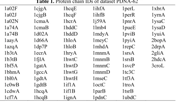
(13) Chapter 2 Materials and Methods 2.1 Datasets We use three datasets (PDNA-62, PDNA-48, PDC-59) to evaluate our SVM-PSSM method which aims to have accurate prediction ability when giving a novel protein with low sequence identity compared with existing samples. Therefore, a filtering tool PISCES with much rigorous definition of sequence identity (Wang and Dunbrack, 2003) is used to filter out highly homologues sequences. Sequence identities for PDB (Protein Data Bank) sequences in PISCES are determined by the combination of CE structural alignment and PSI-BLAST alignment, which is more sophisticated than the traditional local and global alignment method. The sequence identity in PDNA-48 and PDC-59 is confirmed by PISCES. The missed hydrogen of the obtained PDB structures is added by MolProbity (Davis et al., 2004), and it optimizes all hydrogen atoms, both polar and non-polar, on amino acids and nucleic acids. We define the amino acid as a binding residue if its side chain or backbone atoms fell within a cut-off distance 3.5 Å, which is the same as previous study (Ahmad et al., 2004; Ahmad and Sarai, 2005) from any atom on DN. Otherwise, the sample is a non-binding residue. Our calculation result of DNA-Protein binding positions is highly consistent with that of the PDBsum database. PDNA-62: For comparisons, the same dataset PDNA-62, listed in Table 1, containing 62 proteins in previous studies (Ahmad et al., 2004; Ahmad and Sarai, 2005) is used to predict DNA-binding sites in proteins. This dataset consisting of 7967 non-binding and 1792 binding residues has representative protein-DNA complexes from PDB and the protein structure resolution is 2.5 Å or better.. 5.
(14) 1a02F 1a02J 1a02N 1a74A 1a74B 1aayA 1azqA 1b3tA 1b3tB 1bf5A 1bhmA 1bl0A 1c0wB 1cdwA 1cf7A. Table 1. Protein chain IDs of dataset PDNA-62 1cjgA 1hcqE 1ihfA 1perL 1cjgB 1hcqF 1ihfB 1perR 1cmaA 1hcrA 1j59A 1pnrA 1cmaB 1hddC 1lmb4 1pueE 1d02A 1hddD 1mdyA 1pviB 1d66A 1hloA 1meyC 1pyiA 1dp7P 1hloB 1mhdA 1repC 1ecrA 1hryA 1mnmA 1srsA 1fjlA 1hwtC 1mnmB 1srsB 1gatA 1hwtD 1mnmC 1svcP 1gccA 1hwtG 1mnmD 1tc3C 1gdtA 1hwtH 1mseC 1tf3A 1gdtB 1if1A 1octC 1troA 1hcqA 1if1B 1parB 1tsrB 1hcqB 1ignA 1pdnC 1ubdC. 1xbrA 1yrnA 1ysaC 1ysaD 1yuiA 2bopA 2drpA 2gliA 2hdcA 3croL. PDNA-48: The decision boundary in SVM is determined before the prediction that is similar in NN, but in contrast to NN, the overall error function between the predicted and observed class for the training set is minimized, the margin in the boundary is maximized. In other words, the class of a query data at prediction phase is determined according to the established model at training phase. Therefore, the low sequence identity of each protein chain within a dataset would assist the samples in the uniform distribution within the sample space and thus can help the design of classifiers with strong generalization ability. Therefore, PDNA-62 was further filtered by PISCES using an identity threshold 25%. The obtained dataset PDNA-48 contains 48 protein chains (total 6431 residues; 1030 binding residues), listed in Table 2.. 1a02F 1a02N 1a74A 1aayA 1azqA 1b3tA 1bf5A 1bhmA. Table 2. Protein chain IDs of dataset PDNA-48 1bl0A 1gatA 1if1A 1parB 1cdwA 1gccA 1ignA 1pdnC 1cf7A 1gdtA 1ihfA 1pnrA 1cmaA 1hcqA 1j59A 1pueE 1d02A 1hcrA 1lmb4 1pviB 1dp7P 1hloA 1mdyA 1repC 1ecrA 1hryA 1mhdA 1svcP 1fjlA 1hwtC 1mnmA 1tc3C 6. 1troA 1tsrB 1xbrA 1ysaC 1yuiA 2bopA 2hdcA 3croL.
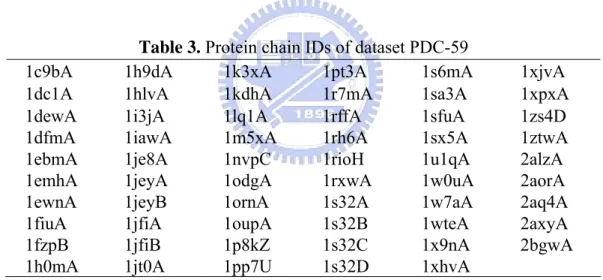
(15) PDC-59: For further evaluating performance of SVM-PSSM in predicting novel proteins, we established a dataset PDC-59 for independent test in this study. These proteins are extracted from the PDB database with released dates after year 2000, and searched by keywords: transcription factor, repressor, regulator, transposase, endonuclease, and DNA-binding. These proteins were also filtered with mutual sequence identity less than 25% compared to each other and to PDNA-48 by PISCES. PDC-59 contains 59 protein chains (total 13041 residues; 1454 binding residues), listed in Table 3. Note that the numbers of binding and non-binding residues in proteins are significantly unequal that the unbalanced distribution should be taken into account in designing accurate predictors.. 1c9bA 1dc1A 1dewA 1dfmA 1ebmA 1emhA 1ewnA 1fiuA 1fzpB 1h0mA. Table 3. Protein chain IDs of dataset PDC-59 1h9dA 1k3xA 1pt3A 1s6mA 1hlvA 1kdhA 1r7mA 1sa3A 1i3jA 1lq1A 1rffA 1sfuA 1iawA 1m5xA 1rh6A 1sx5A 1je8A 1nvpC 1rioH 1u1qA 1jeyA 1odgA 1rxwA 1w0uA 1jeyB 1ornA 1s32A 1w7aA 1jfiA 1oupA 1s32B 1wteA 1jfiB 1p8kZ 1s32C 1x9nA 1jt0A 1pp7U 1s32D 1xhvA. 1xjvA 1xpxA 1zs4D 1ztwA 2alzA 2aorA 2aq4A 2axyA 2bgwA. 2.2 SVM-PSSM 2.2.1 PSSM and feature vector representation in SVM We use multiple sequence alignment profiles generated from PSI-BLAST (Altschul et al., 1997) for each protein chain. We obtain the non-redundant protein sequence database from NCBI (National Center for Biotechnology Information). We set parameters of PSI-BLAST using BLOSUM62 substitution matrix, three iteration runs, and exception value 0.001. The other parameters are set using default values. The PSI-BLAST program by 7.
(16) querying each protein chain against the NCBI NR (Non-Redundant) database is used to generate PSSM profiles which are in the form of 20×N matrix, where N is the length of queried protein chain. Let the residue i be represented by ai = ( ai ,1 ,..., ai ,20 ) where 1 ≤ i ≤ N. Each query residue is represented by a vector of 20 attributes. These profiles are normalized into the range [0, 1] for speeding up the SVM training phase. In the previous study, PSSMs were generated from reference databases with different sizes. Although it was observed that computational time can be saved by replacing the reference database with a much smaller size without loss of much prediction ability (about 2% of NP), we still take the NR database from NCBI as our reference database to make sure that PSI-BLAST can have better multiple sequence alignment results and generate representative PSSMs. The input pattern to SVM using the PSSM features for the residue i is. xi = (ai − k ,..., ai ,..., ai + k ) where k is the number of neighborhood residues on either side. We construct a matrix with window size s=2k+1 centered on the target residue i. The used profile x i is the form of a 20×s matrix. B. B. 2.2.2 SVM SVM is a very popular and powerful method to deal with classification, prediction, and regression problems (Cortes and Vapnik, 1995). The original idea of SVM is to use a linear separating hyperplane which maximizes the distance between two classes to create a classifier. It relies on preprocessing the data to represent patterns in a high dimensional space with an appropriate mapping function φ. For the binary SVM, the training data consist of N pairs (x 1 , B. B. y 1 ), …, (x N , y N ) where instance vectors x i ∈ℜ m and class labels y i ∈{0, 1}, i = 1, …, N. If y i B. B. B. B. B. B. B. B. P. P. B. B. B. B. = 1, x i belongs to the first class; otherwise, x i belongs to the second class. The main task in B. B. B. B. 8.
(17) the training phase is to solve the following optimization problem that seeks a classifier with a maximal margin. The standard formulation of SVM is as follows (Cortes and Vapnik, 1995): N 1 min( w T w + C ∑ ε i ) w , b ,ε i 2 i =1. (1). subject to yi ( w Tϕ ( xi ) + b) ≥ 1 − ε i , ε i ≥ 0 , i = 1,…, N, where w∈ℜ m is a weight vector of training instances and b is a constant. SVM allows sample P. P. i locates at the wrong side of the separating hyperplane w T x + b = 0 with a penalty term ε i , P. P. B. B. and C is a real-value cost parameter for sums of total error. If φ(x i ) = x i , the SVM of (1) finds B. B. B. B. a linear separating hyperplane with a maximal margin. The SVM of (1) is called a nonlinear SVM when φ maps x i into a higher dimensional space. B. B. K(x i , x j ) ≡ φ(x i ) T φ(x j ) is called a kernel function. That is, the dot product in that high B. B. B. B. B. B. P. P. B. B. dimensional space is equivalent to a kernel function of the input space. So we need not be explicit about the transformation φ as long as we know that the kernel function K(x i , x j ) is B. B. B. B. equivalent to the dot product of some other high dimensional space (Vapnik, 1995; Chang and Lin, 2003; Burges, 1998). Some commonly-used kernel functions are exp(-γ|| x i - x j || 2 ) B. B. B. B. P. P. (Radial basis function), (x i T x j /γ+δ) d (Polynomial), and tanh (γx i T x j +δ) (sigmoid), where γ, B. P. PB. B. B. P. P. B. PB. P. B. B. d, and δ are kernel parameters. Chang and Lin (2003) developed a software tool LibSVM (Library for SVM) for support vector classification, including various variants of SVM. The used LibSVM can be found at the website of (Chang and Lin, 2003). In this work, we used K(x i , x j ) = exp(-γ|| x i - x j || 2 ) where the proper values of cost parameter C and kernel B. B. B. B. B. B. B. B. P. P. parameter γ are to be specified. Considering the unbalanced distribution of samples, two additional weight parameters w 0 and w 1 are used to enhance NP performance. The best values of w 0 and w 1 can be B. B. B. B. B. B. B. B. adaptively specified according to the preference on the penalty level for wrong predictions of. 9.
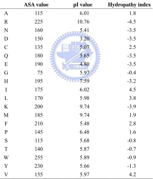
(18) N. non-binding and binding residues, respectively. Therefore, the penalty term C ∑ ε i in (1) is i =1. replaced with C0 ∑ ε i + C1 ∑ ε i , where C0 = w0 × C and C1 = w1 × C (Chang and Lin, yi = 0. yi =1. 2003).. 2.3 Amino acids physico-chemical property features representation As mentioned in earlier researches, nucleotides and amino acids interaction propensity are related to some physico-chemical properties. Therefore, besides of using PSSM profiles as features for classification, we further investigate the performance affected by adding some other amino acids physico-chemical property features in classification. We use SVM which has higher classification performance in this study combines PSSM and each physico-chemical property feature. Ahmad and Sarai (2005) proposed that the probability of binding systematically increased as the proteins solvent accessible surface area (ASA) increased, i.e., the DNA-protein interaction are frequently founded in protein surface than buried fragments (Ahmad and Sarai, 2005). Several researches also analyzed the relation between proteins surface electric charge distribution and DNA-binding propensity, and proposed that some proteins interfaces with DNA are highly enriched in positive charges from lysine and arginine side chains and almost entirely devoid of negative charges from carboxylates (Nadassy et al., 1999). It was also found that the magnitudes of the moments of electric charge distribution in DNA-binding protein chains differ significantly from those of a non-binding control ones (Ahmad and Sarai, 2004). In our study, we use the solvent accessible surface area of amino acids in tripeptide information (Chothia, 1976) and hydropathy index (Kyte and Doolittle, 1982) as the information of tendency that appear in protein surface. The hydropathy index is the scale combining hydrophobicity and hydrophilicity of side chain groups; it can be used to measure 10.
(19) the tendency of an amino acid to seek an aqueous environment or a hydrophobic environment. The amino acids isoelectric point (pI) value is adopted for the residues electric charge information (Zimmerman et al., 1968). The used amino acids physico-chemical properties are listed in Table 4, and their value are also normalized to 0~1 before input to SVM classifier. These physico-chemical properties are tested separately and each of them is integrated to the end of PSSM features; the size of physico-chemical property feature is equal to the used window size: s.. Table 4. List of amino acids physico-chemical properties ASA value. pI value. Hydropathy index. A. 115. 6.01. 1.8. R. 225. 10.76. -4.5. N. 160. 5.41. -3.5. D. 150. 3.20. -3.5. C. 135. 5.07. 2.5. Q. 180. 5.65. -3.5. E. 190. 4.80. -3.5. G. 75. 5.97. -0.4. H. 195. 7.59. -3.2. I. 175. 6.02. 4.5. L. 170. 5.98. 3.8. K. 200. 9.74. -3.9. M. 185. 9.74. 1.9. F. 210. 5.48. 2.8. P. 145. 6.48. 1.6. S. 115. 5.68. -0.8. T. 140. 5.87. -0.7. W. 255. 5.89. -0.9. Y. 230. 5.66. -1.3. V. 155. 5.97. 4.2. 2.4 Evaluation of prediction accuracy In this work, we consider four criteria (Sensitivity, Specificity, net prediction, and 11.
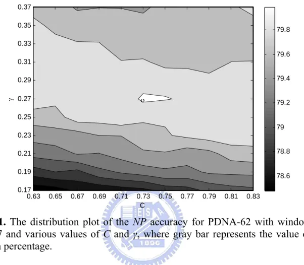
(20) Accuracy) to evaluate the prediction performance. Sensitivity is the percentage of correctly predicted binding residues to total binding residues. Specificity is the percentage of correctly predicted non-binding residues to total non-binding residues. Accuracy is the percentage of correctly predicted residues to total residues. In this study, net prediction (NP, mean of Sensitivity and Specificity) is the first evaluation criterion considering the unbalanced distribution of binding and non-binding residues.. 2.5 Determination of parameter values in SVM In order to advance performance of the SVM classifier for fitting the training datasets with the unbalanced distribution, it is essential to determine the best values of the combination of window size s, cost parameter C, kernel parameter γ, and weight parameters w 0 and w 1 . Since the proper values of s are discrete and limited, we evaluate all candidate B. B. B. B. values of s. A stepwise approach is used to determine the default values of system parameters. At first, the value of w 1 /w 0 is initially set to the ratio of the total number of non-binding B. B. B. B. residues to that of binding residues in the training dataset. For the dataset PDNA-62, w 0 =1.0 B. B. and w 1 =4.446. The best values of parameters C and γ are obtained by maximizing the value B. B. of NP for a prespecified value of s. Here, we use PDNA-62 and perform 6-CV to decide the best values of all system parameters. For example, Fig. 1 is an accuracy distribution plot in terms of NP for various combinations of SVM parameters C and γ with s=7, w 0 =1.0 and B. w 1 =4.446, where the best values of parameters are C=0.73 and γ=0.27. B. B. 12. B.
(21) 0.37 0.35. 79.8. 0.33 79.6 0.31 79.4. γ. 0.29. ο. 0.27. 79.2. 0.25 79 0.23 78.8. 0.21 0.19. 78.6. 0.17 0.63. 0.65. 0.67. 0.69. 0.71. 0.73 C. 0.75. 0.77. 0.79. 0.81. 0.83. Fig. 1. The distribution plot of the NP accuracy for PDNA-62 with window size 7 and various values of C and γ, where gray bar represents the value of NP in percentage. Once the best values of parameters C and γ are obtained in terms of NP, the weights w 0 B. B. and w 1 are then finely tuned using the obtained values of s, C and γ. To enhance the B. B. generalization ability in predicting novel proteins, the values of w 0 and w 1 are determined by B. B. B. B. maximizing the ratio of mean to variance of Sensitivity, Specificity, NP, and Accuracy. Therefore, the SVM classifier is expected to have equivalent performance on classifying binding and non-binding residues. Numerous candidate values of the pair (w 0 , w 1 ) are B. B. B. B. evaluated where w 0 ∈ {0.5, 1.0} and w 1 ∈ {1.0, 50}. Performances of the best SVM classifiers B. B. B. B. with C, γ, w 0 and w 1 for some specified values of window size s using 6-CV on PDNA-62 B. B. B. B. are listed in Table 5.. 13.
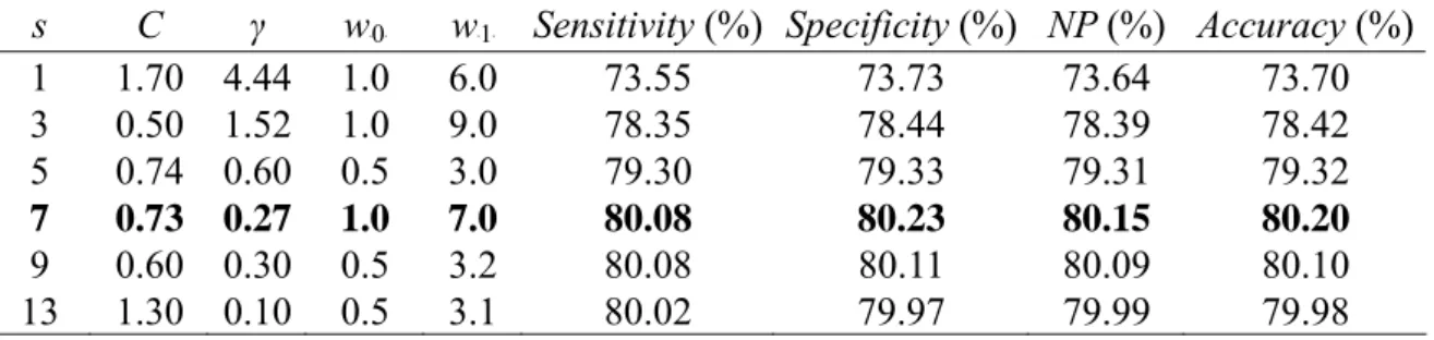
(22) Table 5. Performances of the best SVM classifiers with C, γ, w 0 and w 1 for some specified values of window size s using 6-CV on PDNA-62. w0 w 1 Sensitivity (%) Specificity (%) NP (%) Accuracy (%) s C γ 1 1.70 4.44 1.0 6.0 73.55 73.73 73.64 73.70 3 0.50 1.52 1.0 9.0 78.35 78.44 78.39 78.42 5 0.74 0.60 0.5 3.0 79.30 79.33 79.31 79.32 7 0.73 0.27 1.0 7.0 80.08 80.23 80.15 80.20 9 0.60 0.30 0.5 3.2 80.08 80.11 80.09 80.10 13 1.30 0.10 0.5 3.1 80.02 79.97 79.99 79.98 B. B. B. B. B. B. B. B. Finally, we choose the classifier with parameters s=7, C=0.73, γ=0.27, w 0 =1.0 and B. B. w 1 =7.0 which has the best performance in terms of NP (=80.15%) for the following B. B. independent test. Because there are six classifiers can be obtained using 6-CV, we choose the best one of six classifiers in terms of NP to predict novel proteins. Performances of the best SVM classifier with s=7, C=0.73 and γ=0.27 for some values of w 0 and w 1 on PDNA-62 are B. B. B. B. given in Table 6. The procedure to find best SVM classifier for independent test dataset PDC-59 is listed in Fig. 2.. Table 6. Performances of the SVM classifier with s=7, C=0.73 and γ=0.27 for some values of w 0 and w 1 on the dataset PDNA-62. Sensitivity Specificity NP Accuracy Mean w0 w1 Variance (%) (%) (%) (%) (%) 1.0 2.0 55.86 93.79 74.82 86.82 77.82 827.27 1.0 5.0 76.95 83.24 80.10 82.09 80.60 22.76 1.0 6.0 78.79 81.51 80.15 81.01 80.37 4.25 1.0 6.5 79.41 80.81 80.11 80.55 80.22 1.13 1.0 6.7 79.52 80.62 80.07 80.42 80.16 0.70 1.0 7.0 80.08 80.23 80.15 80.20 80.17 0.01 1.0 8.0 81.31 79.20 80.25 79.59 80.09 2.54 1.0 50 83.98 74.97 79.48 76.63 78.76 46.69 B. B. B. B. B. B. B. B. 14.
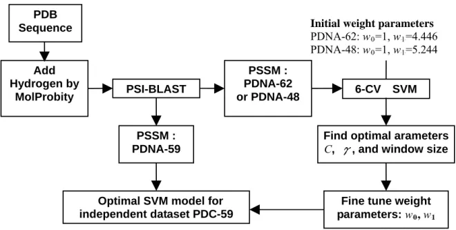
(23) PDB Sequence. Initial weight parameters PDNA-62: w 0 =1, w 1 =4.446 PDNA-48: w 0 =1, w 1 =5.244. Add Hydrogen by MolProbity. PSSM : PDNA-62 or PDNA-48. PSI-BLAST. B. B. B. B. B. B. B. B. 6-CV. SVM. PSSM : PDNA-59. Find optimal arameters C, γ, and window size. Optimal SVM model for independent dataset PDC-59. Fine tune weight parameters: w 0 , w 1 B. B. Fig. 2. The procedure to find the best SVM classifier for independent test.. 15. B.
(24) Chapter 3 Results and Discussion. 3.1 Comparison model: Fuzzy k-NN PSI-BLAST is also used to generate the PSSM profiles as input features for fuzzy k-NN in the form of a 20×L matrix, where L is the length of the sequence. In our study, PSI-BLAST profiles of all protein chains are consistent in fuzzy k-NN and SVM method. We construct a window of size s centered on a target residue, and use the profile that falls within this window, a 20×s matrix, as a feature vector. Then, the distance between two feature vectors A and B is defined as: DAB = ∑ d i Pij( A ) − Pij( B ). (2). i, j. where Pij( A ) (i = 1, 2, …, s; j = 1, 2, …, 20) is a component of the feature vector A, and d i is a neighbor weight parameter. Since we expect the profile elements for residues nearer to B. B. the target residue to be more important in determining the local environment of the target residue, the neighbor weight is defined as: di = (. s +1 s +1 − − i )2 . 2 2. The nearest neighbor algorithm is a friendly to access and widely used classification algorithm. The class of a query data in nearest neighbor algorithm is given according to the classification of those nearest neighbors from a training dataset of known classifications. The general used nearest neighbor algorithm is the so-called k-nearest neighbor algorithm (k-NN), where the query data is assigned the class most frequently represented among the k-nearest samples. The further extension type of k-NN is to give distance weights to the k-nearest samples with a certain power. Furthermore, instead of assigning a definite class to the query data, one can calculate the fuzzy membership, which can be used to estimate the confidence level of the prediction. The algorithm incorporating these generalizations is called the fuzzy k-nearest neighbor algorithm (Fuzzy k-NN) (Keller et al., 1985). 16.
(25) In the fuzzy k-NN method, the fuzzy class membership u i (z) to the class i is assigned to B. B. the query data z according to the following equation:. ∑ u ( z) = i. k. u ( z ( j ) )D jfs. j =1 i k. ∑. D jfs j =1. , i = 1,..., c. where fs = −2 /(m − 1). (3). where m is a fuzzy strength parameter, which determines how heavily the distance is weighted when calculating each neighbor’s contribution to the membership value, k is the number of nearest neighbors, and c is the number of classes. Also, D j which is equivalent to B. B. DAB in function (2) is the distance between the feature vector of the query data z and the feature vector of its j th nearest reference data z (j ) . u i (z (j ) ) is the membership value of z (j ) to the P. P. P. PP. P. B. B. P. PP. P. P. PP. P. i th class, which is 1 if z (j ) belongs to the i th class, and 0 otherwise. Because of the unbalance P. P. P. PP. P. P. P. distribution of samples, one more weight w f is used to enhance NP accuracy, if the reference B. B. ' which is defined as: sample is belong to binding class, DAB is replaced with DAB B. ' DAB =. B. DAB wf. (4). The advantage of the fuzzy k-NN algorithm over the standard k-NN method is clear. The fuzzy class membership u i (z) can be considered as the estimate of the probability that the B. B. query data belongs to class i, and provides us with more information than a definite prediction of the class for the query data. Moreover, the reference samples which are closer to the query data are given more weights, and the optimal value of f s and w f can be chosen B. B. B. B. along with that for k, in contrast to the standard k-NN method with a fixed value of f s = 0. B. B. The optimal value of k, f s , and w f are found from the 6-CV stepwise procedure, and the B. B. B. B. resulting value for f s is indeed nonzero. B. B. Similar to SVM approach, it is important to determine the optimal parameter values of fuzzy k-NN classifier, and there are four parameters in fuzzy k-NN, window size s, number of nearest neighbors k, fuzzy parameter f s , and distance weight w f . The number of nearest B. B. B. B. neighbors k, and window size s, is first prespecified to a fixed value, and the best values of 17.
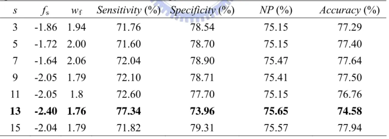
(26) parameters f s and w f are obtained by maximizing the value of NP. When using 6-CV and B. B. B. B. window size: s=13, on PDNA-48, the performance affected by the number of nearest neighbors, k, that increases from 10 to 50 seems less significant. From Table 7, it shows that the NP accuracy only rises slightly from 69.35% to 71.37%. We also investigated the performance affected by window size s from 3 to 15 using 6-CV on PDNA-62. From Table 8, the NP of each model is all around 75% that is not significant improved simultaneously with using larger window size.. Table 7. The performance comparison of fuzzy k-NN classifier with different k value using 6-CV on PDNA-48. NP (%) Accuracy (%) k fs w f Sensitivity (%) Specificity (%) B. B. B. B. 10. -4.90 1.26. 62.14. 76.76. 69.45. 74.42. 30. -2.46 1.72. 72.14. 69.89. 71.02. 70.25. 50. -5.06 1.30. 71.84. 70.89. 71.37. 71.05. Table 8. Performances of the best fuzzy k-NN classifiers with k=30 and f s , w f for some specified values of window size s using 6-CV on PDNA-62. NP (%) Accuracy (%) s fs w f Sensitivity (%) Specificity (%) B. B. B. B. B. B. B. B. 3. -1.86 1.94. 71.76. 78.54. 75.15. 77.29. 5. -1.72 2.00. 71.60. 78.70. 75.15. 77.40. 7. -1.64 2.06. 72.04. 78.90. 75.47. 77.64. 9. -2.05 1.79. 72.10. 78.71. 75.41. 77.50. 11. -2.05. 1.8. 72.60. 77.70. 75.15. 76.76. 13. -2.40 1.76. 77.34. 73.96. 75.65. 74.58. 15. -2.04 1.79. 71.82. 79.31. 75.57. 77.94. From above experiments, it shows that the classification performance of fuzzy k-NN is not affected greatly by window size s and number of nearest neighbors k. Finally, we chose parameter values, s=13 and k=30, that have better classification performance for next independent test on PDC-59.. 18.
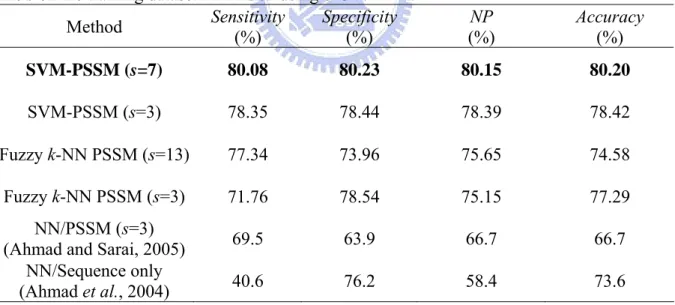
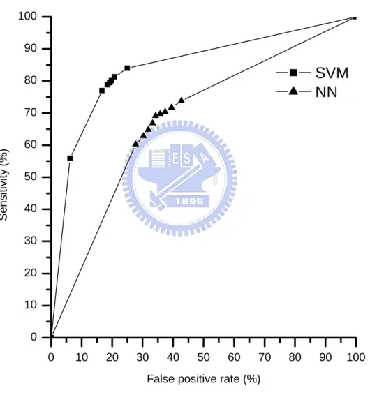
(27) 3.2 Performance comparison of training datasets. To evaluate performance of the proposed method SVM-PSSM and fuzzy k-NN PSSM, the existing NN-based method is conveniently compared using the same 6-CV on PDNA-62. The comparison results are given in Table 9. The NP values of the NN-based methods using sequence information only (Ahmad et al., 2004) and the PSSM feature with window size s=3 (Ahmad and Sarai, 2005) are 58.4% and 66.7%, respectively. The fuzzy k-NN PSSM classifiers with s=3 and 13 have NP=75.15% and 75.65%, respectively. The SVM-PSSM classifiers with s=3 and 7 have NP=78.39% and 80.15%, respectively. The SVM-PSSM classifier is better than the fuzzy k-NN PSSM classifier by increasing the value of NP 4.5% for the training dataset PDNA-62, and much better than the NN-PSSM classifier by increasing the value of NP up to 13.45% for the training dataset PDNA-62.. Table 9. Performance comparison of SVM-PSSM and the NN-based method with window size s on the training dataset PDNA-62 using 6-CV. Sensitivity Specificity NP Accuracy Method (%) (%) (%) (%) SVM-PSSM (s=7). 80.08. 80.23. 80.15. 80.20. SVM-PSSM (s=3). 78.35. 78.44. 78.39. 78.42. Fuzzy k-NN PSSM (s=13). 77.34. 73.96. 75.65. 74.58. Fuzzy k-NN PSSM (s=3). 71.76. 78.54. 75.15. 77.29. 69.5. 63.9. 66.7. 66.7. 40.6. 76.2. 58.4. 73.6. NN/PSSM (s=3) (Ahmad and Sarai, 2005) NN/Sequence only (Ahmad et al., 2004). Besides the NP performance, the Receiver Operating Characteristic (ROC) curve is commonly used to evaluate the discrimination ability of a classifier. The larger area under the ROC curve, the better discrimination ability a classifier has. Fig. 3 gives the performance comparison using the ROC curves on PDNA-62. The ROC curve of the SVM classifier is 19.
(28) obtained from Table 6. The ROC curve of the NN-based classifier is obtained from the DBS-PSSM website as mentioned in (Ahmad and Sarai, 2005). It shows that the area under the ROC curve of SVM is much larger than that of the NN-based method obviously. It also shows that the SVM-based method has better classification ability than the NN-based method in classifying binding and non-binding residues in proteins.. 100 90. SVM NN. 80. Sensitivity (%). 70 60 50 40 30 20 10 0 0. 10. 20. 30. 40. 50. 60. 70. 80. 90. 100. False positive rate (%). Fig. 3. The performance comparison between the SVM and NN-based methods using the ROC curve on PDNA-62.. 3.3 Performance comparison of independent test. In order to evaluate the generalization abilities of the SVM, fuzzy k-NN and NN-based. 20.
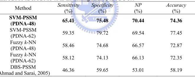
(29) approaches in predicting novel proteins, PDC-59 is used for independent tests. The SVM and fuzzy k-NN classifier are obtained from the best one of 6-CV which has the best NP performance on the training dataset PDNA-62 mentioned above. The results of the NN-based method are obtained through the DBS-PSSM website (Ahmad and Sarai, 2005). Table 10 gives independent test results of three compared methods. The results of SVM, fuzzy k-NN, and NN-based methods are NP=69.54%, 66.13%, and 53.01%, respectively. The SVM classifier is better than the fuzzy k-NN-based method by increasing the NP values for test accuracy up to 3.41%, and much better than the NN-based method by increasing the NP values for test accuracy up to 16.53%. It also reveals that the SVM classifier has better generalization ability to predict novel proteins.. Table 10. Independent test results of the NN-, Fuzzy k-NN-, and SVM-based method (using either PDNA-62 or PDNA-48 as the training dataset) on PDC-59. Sensitivity Specificity NP Accuracy Method (%) (%) (%) (%) SVM-PSSM 65.41 75.48 70.44 74.36 (PDNA-48) SVM-PSSM 59.35 79.72 69.54 77.45 (PDNA-62) Fuzzy k-NN 58.46 74.68 66.57 72.87 (PDNA-48) Fuzzy k-NN 58.12 74.13 66.13 72.35 (PDNA-62) DBS-PSSM 46.36 59.65 53.01 58.19 (Ahmad and Sarai, 2005). To further improve the generalization ability of the SVM classifier, we filter out the proteins with identity greater than 25% in the dataset PDNA-62 by PISCES tool. The obtained dataset PDNA-48 is used as the training dataset. Consequently, we construct the SVM and fuzzy k-NN classifier using the same procedure as that on PDNA-62. The parameters of the obtained SVM classifier from the best one of six classifiers using 6-CV are. s=7, C=0.58, γ=0.23, w 0 =1.0, and w 1 =7.2. The parameters of the obtained fuzzy k-NN B. B. B. B. 21.
(30) classifier are s=13, k=30, f s =-2.46, and w f =1.72. The 6-CV test results of two methods on B. B. B. B. PDNA-48 are listed in Table 11.. Table 11. 6-CV test results of SVM and fuzzy k-NN on PDNA-48.. Method. Sensitivity (%). Specificity (%). NP (%). Accuracy (%). SVM. 75.35. 75.30. 75.32. 75.31. Fuzzy k-NN. 72.14. 69.89. 71.02. 70.25. Table 10 shows that the Sensitivity performance of SVM method is improved from 59.35% to 65.41% and NP performance is slightly improved from 69.54% to 70.44%. The. NP performance of fuzzy k-NN method is slightly improved from 66.13% to 66.57%. Therefore, when we used low identity proteins as training data, it is helpful to obtain a classifier with high generalization ability for correctly predicting binding residues of novel proteins.. 3.4 Analysis and discussion. We further investigate the performance affected by adding some other amino acids physico-chemical property features to classification. We use SVM which has higher classification performance in this study combines PSSM with each physico-chemical property feature. The same procedure as above section is used to find each best SVM model. The 6-CV result of PDNA-48 and parameters of SVM is listed in Table 12, and the independent test on PDC-59 is listed in Table 13.. 22.
(31) Table 12. Performance comparison of SVM method combines PSSM and some physico-chemical features on the training dataset PDNA-48 using 6-CV (s=7). Sensitivity Specificity NP Accuracy Features C γ w0 w1 (%) (%) (%) (%) B. B. B. B. PSSM. 0.58 0.23 1.0 7.2. 75.35. 75.30. 75.33. 75.31. PSSM + ASA. 0.69 0.16 1.0 6.5. 75.25. 75.43. 75.34. 75.40. PSSM + pI. 0.27 0.27 1.0 6.5. 75.54. 74.00. 74.77. 74.25. PSSM + hydropaty index. 1.2 0.12 1.0 7.5. 74.57. 73.87. 74.22. 73.99. Table 13. Independent test result of PDC-59 using PDNA-48 as training data (s=7).. Features PSSM PSSM + ASA PSSM + pI PSSM + hydropaty index. Sensitivity (%) 65.41 65.96 65.27 66.71. Independent test (PDC-59) Specificity NP (%) (%) 75.48 70.44 76.14 71.05 75.56 70.41 74.32. 70.58. Accuracy (%) 74.36 75.00 74.41 73.48. It shows that PSSM combines with amino acids physico-chemical properties dose not further improve the NP accuracy, only at the condition that PSSM combines ASA feature slightly promote the NP accuracy of independent test from 70.44% to 71.05%. Although previous researches proposed that these amino acids physico-chemical properties are related to DNA-proteins interactions, the further well design of combining PSSM and physico-chemical property features seems needed to enhance the classification accuracy. The process of DNA-protein recognition is flexible and continuous (Gunther et al., 2006; Sarai and Kono, 2005), and the crystals of protein-DNA complex just catch a moment of this whole process. Therefore, the amino acid defined as a non-binding residue with a distance slightly larger than the cut-off distance 3.5 Å may assist or take part in protein-DNA recognition. We analyze the distance distribution of non-binding residues in PDC-59 which 23.
(32) are incorrectly classified as binding ones by the SVM classifier using the training dataset PDNA-48. The result given in Fig. 4 reveals that there are 39% of non-binding residues with the distance in the range 3.5~8.5 Å close to the nearest DNA nucleotide. The percentage of misclassified non-binding residues decreases gradually when their distance increases. The logical result reveals that SVM-PSSM is a good predictor for biologist to analyze the protein-DNA-binding mechanism.. 40 35 30. %. 25 20 15 10 5 0 3.5~8.5. 8.5~13.5 13.5~18.5 18.5~23.5 23.5~28.5 28.5~33.5 33.5~38.5. >38.5. Angstrom. Fig. 4. Distance distribution of misclassified non-binding residues. X-axis represents the distance between the residues to the nearest atom on DNA. Y-axis represents the percentage of misclassified non-binding residues to total non-binding residues in the specified distance range. The class of a query residue is determined by the discrimination function of SVM. When the function value of a residue is greater than zero, it would be classified into the non-binding class. Otherwise, it would be classified into the binding class. Fig. 5 shows the relationship of discrimination function values and distances between the residues to the nearest atom on 24.
(33) DNA using all misclassified non-binding residues. It reveals that these misclassified non-binding residues which are closer to DNA would get smaller values of the SVM discrimination function. This scenario indicates that the SVM classifier has good screening abilities to select potential binding residues. These amino acids with distances in the vague region may potentially take part in or assist protein-DNA recognition and can be further verified by biologist.. 0.0. Discrimination function value. -0.5. -1.0. -1.5. -2.0. -2.5. 5. 10. 15. 20. 25. 30. 35. 40. 45. 50. 55. 60. 65. 70. Angstrom. Fig. 5. Relationship of discrimination function values and distances between the residues to the nearest atom on DNA using all misclassified non-binding residues. In our study, the SVM method has higher performance than fuzzy k-NN method. Fuzzy k-NN method assigns the query data to a class according to the k nearest neighbors classes and distances to the query data, and SVM method assigns the query data to a class according to established model from training data. When two classes of data spread in sample space. 25.
(34) with higher overlapping, fuzzy k-NN method should own more advantage than SVM method. But the obvious unbalance data distribution in this study shows that much of the binding class data is surrounded by non-binding class. Fig. 6 is the statistic plot of numbers of neighbors with the same class in 30 nearest neighbors that reveals the situation mentioned above, the non-binding class data always have much neighbors with the same class, but it is a different situation in binding class data. SVM maps the original features to higher dimensional space by a kernel function seems more efficiently separate two class of data than fuzzy k-NN.. 1600. Non-binding Binding. 1400 1200. Samples. 1000 800 600 400 200 0 0. 5. 10. 15 20 Number of neighbors with the same class as a query data. 25. 30. Fig. 6. Number of neighbors with the same class as a query data in 30 nearest neighbors in fuzzy k-NN method using PDNA-48 as training data and PDC-59 as test data.. 26.
(35) 30 Binding Non-binding 25. (%). 20. 15. 10. 5. 0 -4. -3. -2. -1. 0. 1. 2. 3. 4. Discrimination function value. Fig. 7. Data distribution of binding and non-binding residues in PDC-59 using the SVM classifier. Generally, the cut-off value of SVM discrimination function is set to zero for normal classification. Fig. 7 shows the distribution of binding and non-binding residues in PDC-59 using the SVM classifier with a cut-off value equal to zero. Once the SVM classifier with the best setting of parameters (s, C, γ, w 0 , w 1 ) is developed, we may adjust the cut-off value in B. B. B. B. using the SVM classifier according to the preference such as higher NP, higher Sensitivity, higher Specificity, etc. Table 14 gives the result of the SVM classifier (s=7, C=0.58, γ=0.23,. w 0 =1.0, and w 1 =7.2) on the dataset PDC-59 for various cut-off values. For example, if the B. B. B. B. cut-off value is set to 0.29, the highest value of NP equals to 71.15%. If the higher Sensitivity performance is desirable, the cut-off value of the SVM classifier can be properly increased.. 27.
(36) Table 14. Results of the best SVM classifier (s=7, C=0.58, γ=0.23, w 0 =1.0, and w 1 =7.2) on the dataset PDC-59 for various cut-off values. Sensitivity (%) Specificity (%) NP (%) Accuracy (%) Cut-off value -3.00 0.00 100.00 50.00 88.84 -2.00 1.93 99.84 50.88 88.91 -1.00 24.28 96.05 60.16 88.04 -0.50 44.02 88.17 66.09 83.24 -0.30 53.09 83.85 68.47 80.42 -0.10 61.97 78.69 70.33 76.82 0.00 65.41 75.48 70.44 74.36 0.10 69.33 72.00 70.66 71.70 0.13 70.70 70.92 70.81 70.89 0.29 77.10 65.19 71.15 66.52 0.30 77.44 64.75 71.10 66.16 0.50 83.77 56.80 70.28 59.80 1.00 94.09 35.20 64.64 41.77 2.00 99.31 6.32 52.81 16.68 3.00 100.00 0.20 50.10 11.32 B. 28. B. B. B.
(37) Chapter 4 Conclusions In our study, we have proposed a hybrid method using SVM in conjunction with the PSSM features for prediction of DNA-binding sites in proteins from amino acid sequences by achieving high accuracy for novel proteins. Using the same PSSM features, simulation results show that our method SVM-PSSM is better than fuzzy k-NN method and much better than the existing neural network based method in terms of net prediction (NP) accuracy by increasing the NP values for training and test accuracies up to 13.45% and 16.53%, respectively. Although previous researches proposed that amino acids physico-chemical properties such as ASA, electric charge, and hydropathy are related to DNA-proteins interactions, when using PSSM combines these physico-chemical properties as features, they only keep the original performance. It seems that the further well design of combining PSSM and physico-chemical properties features are needed to enhance the performance. To best of our knowledge, up to now, the proposed method is the most effective method for recognizing mechanism of binding residues in proteins based on protein sequence without using 3D structural information, such as hydrogen bond, hydrophobic, hydrophilic, ion interaction, etc. By adjusting the cut-off value of the SVM classifier, the proposed prediction method would be helpful to biologist for filtering novel proteins without significant homology with known protein to find out the potential binding regions in proteins.. 29.
(38) References Ahmad, S., Gromiha, M.M., Sarai, A., 2004. Analysis and prediction of DNA-binding proteins and their binding residues based on position, sequence and structural information. Bioinformatics 20, 477-486. Ahmad, S., Sarai, A., 2004. Moment-based Prediction of DNA-binding Proteins. Journal of. Molecular Biology 341, 65-71. Ahmad, S., Sarai, A., 2005. PSSM-based prediction of DNA-binding sites in proteins. BMC. Bioinformatics 6, 33. Altschul, S.F., Madden, T.L., Schaffer, A.A., Zhang, J.H., Zhang, Z., Miller, W., Lipman, D.J., 1997. Gapped BLAST and PSI-BLAST: a new generation of protein database search programs. Nucleic Acids Research 25, 3389-3402. Ansari, A.Z., Mapp, A.K., 2002. Modular design of artificial transcription factors. Current. Opinion in Chemical Biology 6, 765-772. Bhardwaj, N., Langlois, R.E., Zhao, G.J., Lu, H., 2005. Kernel-based machine learning protocol for predicting DNA-binding proteins. Nucleic Acids Research 33, 6486-6493. Blancafort, P., Segal, D.J., Barbas, C.F., 2004. Designing Transcription Factor Architectures for Drug Discovery. Molecular Pharmacology 66, 1361-1371. Burges, C.J.C., 1998. A Tutorial on Support Vector Machines for Pattern Recognition. Data. Mining and Knowledge Discovery 2, 121-167. Chang, C.C., Lin, C.J. 2003. LIBSVM: a library for support vector machines. Software. available at http://www.csie.ntu.edu.tw/~cjlin/libsvm. Chen, Y.C., Hwang, J.K., 2005. Prediction of disulfide connectivity from protein sequences.. PROTEINS: Structure, Function, and Bioinformatics 61, 507-512. Cheng, A.C., Chen, W.W., Fuhrmann, C.N., Frankel, A.D., 2003. Recognition of Nucleic Acid Bases and Base-pairs by Hydrogen Bonding to Amino Acid Side-chains. Journal of 30.
(39) Molecular Biology 327, 781-796. Chothia, C., 1976. The nature of the accessible and buried surfaces in proteins. Journal of. Molecular Biology 105, 1-12. Cortes, C., and Vapnik, V. 1995. Support-vector network. Machine Learning 20, 273-297. Davis, I.W., Murray, L.W., Richardson, J.S., Richardson, D.C., 2004. MolProbity: structure validation and all-atom contact analysis for nucleic acids and their complexes. Nucleic. Acids Research 32, W615-W619. Frishman, D., Mewes, H.W., 1997. PEDANTic genome analysis. Trends in Genetics 13, 415-416. Gunther, S., Rother, K., Frommel, C., 2006. Molecular flexibility in protein-DNA interactions.. Biosystems (in press) Guo, J., Chen, H., Sun, Z.R., Lin, Y.L., 2004. A Novel Method for Protein Secondary Structure Prediction Using Dual-Layer SVM and Profiles. PROTEINS: Structure,. Function, and Bioinformatics 54, 738-743. Huang,Y., Li,Y., 2004. Prediction of protein subcellular locations using fuzzy k-NN method.. Bioinformatics 20, 21-28. Kel, A.E., Gossling, E., Reuter, I., Cheremushkin, E., Kel-Margoulis, O.V., Wingender, E., 2003. MATCH: a tool for searching transcription factor binding sites in DNA sequences.. Nucleic Acids Research 31, 3576-3579. Keller, J.M., Gray, M.R., Givens, J.A, 1985. A fuzzy k-nearest neighbor algorithm. IEEE. Transaction on Systems, Man and Cybernetics 15, 580-585. Kyte, J., Doolittle, R.F., 1982. A simple method for displaying the hydropathic character of a protein. Journal of Molecular Biology 157, 105-132. Lejeune, D., Delsaux, N., Charloteaux, B., Thomas, A., Brasseur, R., 2005. Protein-Nucleic Acid Recognition: Statistical Analysis of Atomic Interactions and Influence of DNA. 31.
(40) Structure. PROTEINS: Structure, Function, and Bioinformatics 61, 258-271. Luscombe, N.M., Austin, S.E., Berman, H.M., Thornton, J.M., 2000. An overview of the structures of protein-DNA complexes. Genome Biology 1, 1-10. Luscombe, N.M., Thornton, J.M., 2002. Protein-DNA Interactions: Amino Acid Conservation and the Effects of Mutations on Binding Specificity. Journal of Molecular Biology 320, 991-1009. Nadassy, K., Wodak, S.J., Janin, J., 1999. Structural Features of Protein-Nucleic Acid Recognition Sites. Biochemistry 38, 1999-2017. Natt, N.K., Kaur, H., Raghava, G.P.S., 2004. Prediction of transmembrane regions of β-barrel proteins using ANN- and SVM-based methods. PROTEINS: Structure, Function, and. Bioinformatics 56, 11-18. Nguyen, M.N., Rajapakse, J.C., 2005. Prediction of Protein Relative Solvent Accessibility With a Two-Stage SVM Approach. PROTEINS: Structure, Function, and Bioinformatics 59, 30-37. O’Flanagan, R.A., Paillard, G., Lavery, R., Sengupta, A.M., 2005. Non-additivity in protein-DNA-binding. Bioinformatics 21, 2254-2263. Pabo, C.O., Nekludova, L., 2000. Geometric Analysis and Comparison of Protein-DNA Interfaces: Why is there no Simple Code for Recognition?. Journal of Molecular. Biology 301. 597-624. Paul, T.K., Iba, H., 2006. Gene selection for classification of cancers using probabilistic model building genetic algorithm. Biosystems 82, 208-205. Pudimat, R., Schukat-Talamazzini, E.G., Backofen, R., 2005. A multiple-feature framework for modeling and predicting transcription factor binding sites. Bioinformatics 21, 3082-3088. Sarai, A., Kono, H., 2005. Protein-DNA Recognition Patterns and Predictions. Annual Review. 32.
(41) of Biophysics and Bimolecular Structure 34, 379-398. Sim, J., Kim, S.Y., Lee, J. 2005. Prediction of protein solvent accessibility using fuzzy. k-nearest neighbor method. Bioinformatics 21, 2844-2849. Segal, D.J., Barbas, C.F., 2001. Custom DNA-binding proteins come of age: polydactyl zinc-finger proteins. Current Opinion in Biotechnology 12, 632-637. Stawiski, E.W., Gregoret, L.M., Mandel-Gutfreund, Y., 2003. Annotating Nucleic Acid-Binding Function Based on Protein Structure. Journal of Molecular Biology 326, 1065-1079. Vapnik, V., 1995. The nature of statistical learning theory. Springer-Verlag, New York. Wang, G.L., Dunbrack, R.L., 2003. PISCES: a protein sequence culling server. Bioinformatics 19, 1589-1591. Wingender, E., Chen, X., Hehl, R., Karas, H., Liebich, I., Matys, V., Meinhardt, T., Pruss, M., Reuter, I., Schacherer, F., 2000. TRANSFAC: an integrated system for gene expression regulation. Nucleic Acids Research 28, 316-319. Yaghmai, R., Cutting, G.R., 2002. Optimized Regulation of Gene Expression Using Artificial Transcription Factors. Molecular Therapy 5, 686-694. Zimmerman, J.M., Eliezer, N., Simha, R., 1968. The characterization of amino acid sequences in proteins by statistical methods. Journal of theoretical biology 21, 170-201.. 33.
(42)
數據
+7
Outline
相關文件
• The start node representing the initial configuration has zero in degree.... The Reachability
We do it by reducing the first order system to a vectorial Schr¨ odinger type equation containing conductivity coefficient in matrix potential coefficient as in [3], [13] and use
• Content demands – Awareness that in different countries the weather is different and we need to wear different clothes / also culture. impacts on the clothing
• Examples of items NOT recognised for fee calculation*: staff gathering/ welfare/ meal allowances, expenses related to event celebrations without student participation,
We propose a primal-dual continuation approach for the capacitated multi- facility Weber problem (CMFWP) based on its nonlinear second-order cone program (SOCP) reformulation.. The
Monopolies in synchronous distributed systems (Peleg 1998; Peleg
Corollary 13.3. For, if C is simple and lies in D, the function f is analytic at each point interior to and on C; so we apply the Cauchy-Goursat theorem directly. On the other hand,
• We shall prove exponential lower bounds for NP-complete problems using monotone circuits. – Monotone circuits are circuits without
