A High-Definition H.264/AVC Intra-Frame Codec IP
for Digital Video and Still Camera Applications
Chun-Wei Ku, Chao-Chung Cheng, Guo-Shiuan Yu, Min-Chi Tsai, and Tian-Sheuan Chang, Member, IEEE
Abstract—This paper presents a real-time high-definition
720p@30fps H.264/MPEG-4 AVC intra-frame codec IP suitable for digital video and digital still camera applications. The whole design is optimized in both the algorithm and architecture levels. In the algorithm level, we propose to remove the area-costly plane mode, and enhance the cost function to reduce hardware cost and to increase the processing speed while provide nearly the same quality. In the architecture design, in additional to the fast module implementation the process is arranged in the macroblock-level pipelining style together with three careful scheduling techniques to avoid the idle cycles and improve the data throughput. The whole codec design only needs 103 K gate count for a core size of 1.28 1.28 mm2and achieves real-time encoding and decoding at 117 and 25.5 MHz, respectively, when implemented by 0.18- m CMOS technology.
Index Terms—High definition, intra-frame codec, ISO/IEC
14496-10 AVC, ITU-T Rec. H.264, Joint Video Team (JVT).
I. INTRODUCTION
W
ITH the demand of higher video quality, lower bit rate, and feasibility of fast growing semiconductor processing, a new video coding standard is developed by the Joint Video Team (JVT) of ISO/IEC MPEG and ITU-T VCEG as the next generation video compression standard, which is known as H.264 or MPEG-4 Part 10 Advanced Video Coding (MPEG-4 AVC) [1]. Comparing with previous MPEG-2 and MPEG-4 video standards, the latest H.264 video coding can improve the coding efficiency by up to 50% with various newly introduced coding tools [2]. These new tools include the simpli-fied transform, variable block-size motion compensation, and context adaptive entropy coding. A new intra-frame prediction technique is also introduced to use neighboring pixel values to predict currently coding block, instead of the simple dc/ac predictions in MPEG-4. The intra-frame coding capability in H.264 can achieve higher coding efficiency than that in the previous standards and even competitive with the latest still image coding standard, JPEG2000 [3]. Thus, this intra-only Manuscript received December 7, 2005; revised April 24, 2006. This work was supported in part by the National Science Council, Taiwan, R.O.C., under Grant NSC-93-2200-E-009-028. This paper was recommended by Associate Editor K.-H.Tzou.C.-W. Ku is with MediaTek, Inc., Hsinchu 300, Taiwan, R.O.C.
C.-C. Cheng is with the Graduate Institute of Electronics Engineering, Na-tional Taiwan University, Hsinchu 300, Taiwan, R.O.C.
G.-S. Yu is with Faraday Technology Inc., Hsinchu 300, Taiwan, R.O.C. M.-C. Tsai is with Andes Technology Inc., Hsinchu 300, Taiwan, R.O.C. T.-S. Chang is with the Department of Electronics Engineering, Na-tional Chiao Tung University, Hsinchu 300, Taiwan, R.O.C. (e-mail: [email protected]).
Color versions of Figs. 3, 6–10, 14, and 15 are available online at http://iee-explore.ieee.org.
Digital Object Identifier 10.1109/TCSVT.2006.879992
coding and decoding is very suitable for applications like digital video recorder and digital still camera that do not need or cannot afford the inter prediction capability.
In this paper, we present an H.264 intra-frame codec IP chip that can be configured as both encoder and decoder. The chip combines and shares encoder and decoder hardware resources for lower area cost. The design is optimized from algorithm level to architecture level for hardware implementation. In the intra-codec process, the intra-prediction occupies most of the computing cycles, in which the plane mode implemen-tation occupies significant cycle count and half of area of intra-predictor. Thus, in the hardware oriented algorithm level optimization, we try to eliminate the plane mode usage. How-ever, direct removal will cause quality degradation. Therefore, we propose an enhanced cost function to improve the quality a little bit first to compensate the quality loss of plane mode removal. This algorithm optimization significantly reduces the required processing cycles in hardware and saves almost half of intra-prediction hardware and buffer cost with negligible quality loss. Furthermore, in the architecture level, we balance the processing speed of hardware design by macroblock level pipelining, and minimize its idle cycles by three scheduling techniques. The area cost and processing speed are further optimized by the bottom module designs, like reconfigurable intra-prediction datapath and zero-skipped context adaptive variable length coding (CAVLC) codec. Besides, the decoding process can easily fit into the encoding one with additional CAVLC decoder, a few multiplexers, and buffers due to mod-ularized design approaches. The final chip implementation can achieve real-time high-defintion (HD) sized encoding and decoding with low hardware cost and operating frequency.
This paper is organized as follows. In Section II, we first briefly take an overview of H.264 intra-coding and decoding flow. Then, we present our algorithm-level optimizations to fit the hardware design in the concern of cost and quality in Section III. Section IV shows the entire codec architecture and its detailed component designs. The experimental results of implementation and comparison with other H.264 encoder or decoder are shown in Section V. Finally, a conclusion remark is given in Section VI.
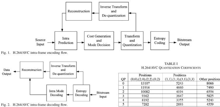
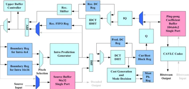
II. OVERVIEW OFH.264 INTRA-CODING ANDDECODING Figs. 1 and 2 show the intra-frame encoding flow and de-coding flow of H.264 [1], respectively. To encode a macroblock in the intra-frame, the process first performs the intra-mode pre-diction. Then the prediction mode with minimum cost value is chosen as the best mode by cost generation and mode decision function. Residuals after the prediction are further processed by the forward transform, quantization, dequantization, inverse 1051-8215/$20.00 © 2006 IEEE
Fig. 1. H.264/AVC intra-frame encoding flow.
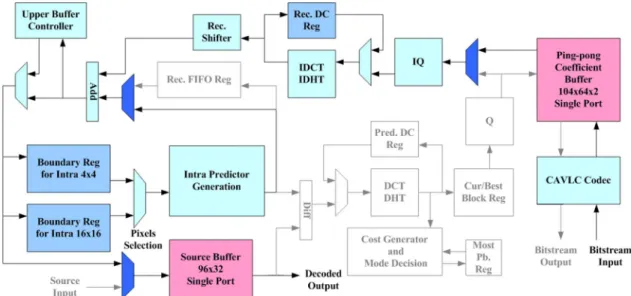
Fig. 2. H.264/AVC intra-frame decoding flow.
transform, and finally reconstructed as reference for next mac-roblock processing. Besides, the coefficients after quantization and mode information are handled by entropy coding, CAVLC and universal variable length coding (UVLC). On the contrary, the decoding process recovers residuals through CAVLC de-coder, dequantization, and inverse transform in the proper order. With residuals, decoded macroblocks can be reconstructed by adding them to predicted data according to the mode informa-tion. For details, see [1].
A. Intra-Prediction
The intra-prediction modes for the luma components can be one of nine 4 4 modes or one of four 16 16 modes. These intra-prediction modes will use the neighboring boundary pixels of upper and left blocks as the reference. The prediction process is the performance bottleneck in hardware design of encoder since prediction for the next block has to wait for the recon-structed reference samples from feedback loop. Similar proce-dures are also applied to the chroma components.
B. Cost Generation and Mode Decision
The best mode decision of intra-prediction1can be either the
time consuming rate distortion optimization (RDO) or just much simpler sum of absolute transform difference (SATD) of each 4
4 block defined as follows:
For most probable mode (1)
For other modes) (2) (3) 1H.264/MPEG-4 AVC Reference Software JM8.6
TABLE I
H.264/AVC QUANTIZATIONCOEFFICIENTS
where denotes the lambda values which are derived from the approximate exponential function depending on the quanti-zation parameters, and and are the th elements of source block and predicted block, respectively. Since there are 52 quantization parameters, there are total 52 related lambda values. In addition, the function in (3) represents the 4 4 discrete Hadamard transform (DHT), as shown in (4), where the matrix means the residual matrix
(4)
C. Transform and Quantization
In H.264, an approximated 4 4 discrete cosine transform (DCT) is used. It can be divided into two parts, 4 4 integer transform and fractional scalar multiplication factors that are further merged into the quantization stage. The forward 4 4 integer transform with quantization is illustrated in (5), and the inverse one with dequantization is illustrated in (6). In which, the matrices with factors and denote the scalar multiplica-tion. The dc values of sixteen blocks will be further processed by 4 4 DHT or 2 2 DHT for the 16 16 and 8 8 intra-predic-tions. The data after transformed are then quantized by integer quantization.
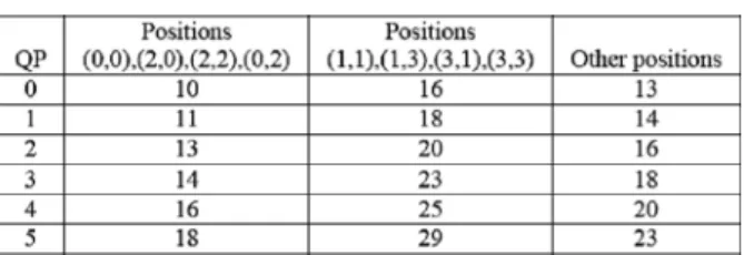
In the quantization stage, there are 52 values of quantization parameters and corresponding quantization steps supplied in H.264 standard. The scaling factors mentioned above are incor-porated into these quantization coefficients. These coefficients are implemented in the reference software as multiplication ta-bles shown in Tata-bles I and II. After this stage, the quantized data
TABLE II
H.264/AVC DEQUANTIZATIONCOEFFICIENTS
is sent to not only entropy coding unit but feedback loop to be reconstructed
(5)
(6)
D. Entropy Coding
In baseline profile, standard uses CAVLC for coding the quantized samples to bit stream. The following items are coded in a proper order: number of nonzero coefficients, sign marks of trailing ones, levels of remaining nonzero coefficients, number of total zeros, and runs of zeros between nonzero coefficients. The decoding process is the reverse of the encoding one. For encoding process, the coefficients should be first scanned in the reversed zigzag order before coding.
III. HARDWAREORIENTEDALGORITHMOPTIMIZATION
A. Enhanced SATD Cost Function for Mode Decision
In determining the coding performance of intra-only H.264, the cost function for mode decision is the most important part. In which, though RDO can provide the best performance, its com-plexity hinders its use in the hardware design. Thus, the SATD method is adopted. However, how to determine the transform for SATD computation will become the main issue now. The trans-form choice used in SATD should be computationally simple
but also effective to estimate the energy of the signals. Thus, in the reference software , the 4 4 DHT is adopted, but it is far from the real transform in the whole encoding process. A better choice for SATD shall approximate the effect of transform and quantization as that used in H.264 encoding to estimate the real bit rate. Therefore, previous designs [4], [5] use the 4 4 integer transform as the choice. Although their approaches can achieve better performance than DHT does, it is still not good enough since the fractional multiplication factors do not be taken into consideration. A complete transform function in H.264 shall in-clude both the integer transform and multiplication factors in the quantization formula as shown in (5). However, to incorpo-rate these factors into the cost function directly will cost a lot of computation since they are not simple numbers for computa-tion. Besides, these factors cannot be directly derived from (5) since the quantization coefficients shall also be included.
To solve the problems, we propose a new cost function that combines the integer transform and simplified multiplication factors. The simplified factors are derived from quantization co-efficients shown in Tables I and II. Derivation from the quantiza-tion coefficients enables us to consider both the effect of trans-form and quantization. From these tables, we can obtain the quired factors by approximating the relationship among the re-ciprocal of dequantization coefficients and simplifying them to be computationally simple as
(7) (8) where the symbols represent the quantization and de-quantization coefficients of different positions in Tables I and II. These simplified scaling factors from inverse quantization are adopted as shown in (9) by considering the final performance and implementation cost. In the formula, division by 32 is added to avoid the enlargement of the cost values, which can be car-ried out with simple wiring to reduce computational complexity as well as hardware cost. Therefore, this cost function is able to estimate the energy of residuals after the transform more accu-rate than other methods while keeps computation simple and suitable for hardware implementation. Besides, it can provide better quality than that in the reference software and can be used to compensate the quality loss of plane mode removal discussed in the next subsection.
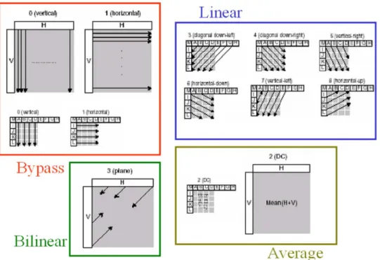
Fig. 3. Four categorized types of intra-luma prediction modes. TABLE III
PROBABILITYDISTRIBUTION OFALL162 16 MODES INDIFFERENT
SEQUENCESWITH300 I-FRAMESWHENQP = 28
B. Plane Mode Removal
The various intra-prediction modes can further be organized systematically into four types according to their prediction prop-erties and computation complexity. These four types of intra-luma prediction modes are illustrated in Fig. 3: bypass, average, linear, and bilinear type. The bypass type is easy to be imple-mented since the prediction samples are the same as boundary pixels. In average type, neighboring eight pixels (for 4 4 prediction) or 32 pixels (for 16 16 prediction) are summa-rized and divided to generate an average value for all prediction samples. The linear type contains most of the 4 4 prediction modes with directional approach, and the samples are linearly interpolated from boundary pixels. Finally, in the bilinear type, also known as plane mode, samples are derived by the approxi-mation of bilinear function. Though being simplified to be only integer arithmetic operations, the plane mode is still much more computationally complex than other modes, hard to reuse its re-sults for other prediction, and occupies almost half of the area in intra-prediction unit.
A solution for this problem is to eliminate the plane mode from the intra-prediction and replace it with other modes. This may raise the issue of performance loss. Table III shows the probability distribution of all 16 16 prediction modes. The macroblocks predicted in plane mode is only 4.2% in average
and generally not larger than 5.7% except the sequence “Akiyo” which contains smooth image. However, after simulation we find that the intra-prediction with plane mode only reduces about 1% of bit rate than that without plane mode for those video sequences. The loss of 1% bit rate difference can be easily compensated by the proposed enhanced cost function. With this, we can achieve almost the same results as the original one but save lots of computational cycles and area cost.
C. Simulation Results
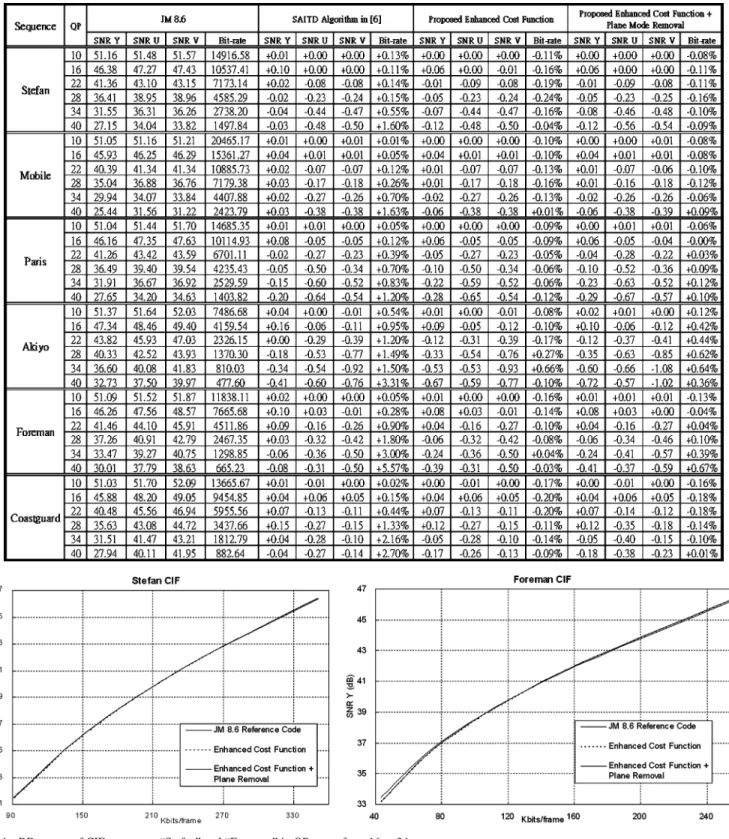
Table IV illustrates the comparison results for encoding of six CIF-size sequences with all intra-frames in different quantiza-tion parameters (QP) among four algorithms: the original ref-erence software , SAITD algorithm in [5], proposed enhanced cost function, and the previous one combining with plane mode removal. In most cases of the simulation, it is obvious that the proposed cost function is able to achieve better coding efficiency than or [5] does, with almost the same or even better PSNR. We can also observe that the proposed algorithm can reduce average 0.08% bit rate for all sequences. After combining with technique of plane mode removal, the bit rate increase is compensated and not larger than 0.06% in average. Fig. 4 shows two rate-distor-tion (RD) curves of sequences “Foreman” and “Stefan,” where QP range is from 16 to 34. The curves of proposed algorithm are very close to those from reference code and even better in the high bit rate coding. The algorithm-level optimization makes the final hardware design not only simpler but also with good video quality.
IV. ARCHITECTUREDESIGN
A. Analysis of Hardware Complexity
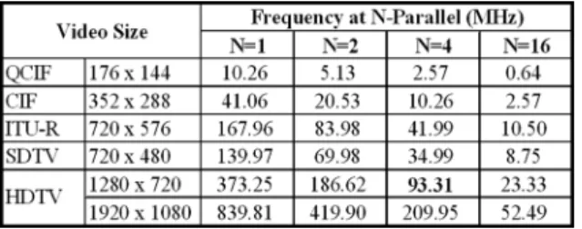
To achieve the target throughput for our target of video appli-cation, HD 720p (1280 720 at 30 fps), the complexity of hard-ware shall be first analyzed before design. Table V shows the
TABLE IV
COMPARISONBETWEEN THEORIGINAL, PREVIOUSALGORITHM[5],ANDPROPOSEDALGORITHM IN300 INTRA-FRAMES
Fig. 4. RD curves of CIF sequences “Stefan” and “Foreman” in QP range from 16 to 34.
data throughput requirement in different video sizes at 30 fps. Thus, our design is required to have the ability to sequentially carry out the data throughput of at least 108,000 macroblocks/s, which is identical to 27.65 Mpixels/s.
To estimate the required operating frequency for hardware design, we start the exploration of the computation cycles for intra-prediction. We simplify this problem by neglecting the
cycles of data transfer between on-chip and off-chip memory, and assuming that only prediction cycles are performed. With such assumption, the total cycle count for predicting one set of macroblocks in encoding process, including one luma and two chroma components, is
, where plane modes are removed and extra setup cycles are excluded,) and the related frequency is 373.25 MHz
TABLE V
DATATHROUGHPUTREQUIREMENT FORDIFFERENTVIDEOSIZE
TABLE VI
OPERATINGFREQUENCY FORN-PIXELPARALLELENCODER
TABLE VII
OPERATINGFREQUENCY FORN-PIXELPARALLELDECODER
for 720p video size with processing of one pixel at a time. This speed requirement is far beyond the generally acceptable range and hard to be implemented.
As a consequence, the design skill such as parallelism is ap-plied to reduce the operating frequency. Tables VI and VII show the estimation results of encoder and decoder for such pixel par-allelism, respectively. For encoder design, the suitable choice is to use the four-pixel parallel architecture that operates at fre-quency of 93.31 MHz and needs 864 cycles for one macroblock. With this, the corresponding four-pixel parallel decoder only needs 96 cycles at 10.37 MHz to decode a macroblock. Such design target can achieve the real-time requirement while is still easy to be implemented.
B. Macroblock Level Pipelining
Previous estimation only assumes the cycle for intra-predic-tion. However, more cycles will be needed when considering other functions like data transfer between memories and entropy coding. These necessary operations will increase the total cycle count to complete the coding of a macroblock and thus results in higher operating frequency. For example, the CAVLC circuit in [6] takes about 500 cycles to encode a high-quality application video. This will increase the latency to around 1,400 cycles and with the frequency to 150 MHz. In addition, the zigzag scan in
Fig. 5. Proposed ping-pong architecture with macroblock-level pipelining.
CAVLC unit will also increase the cycles since its order is quite different than the raster scan order used in the prediction engine. To solve above problems, we use the macroblock-level pipelining as shown in Fig. 5. This pipelining enables the overlapped execution of intra-prediction and entropy coding without large cycle increases. After pipelining, the cycle number of a macroblock depends on the longest latency of each processing unit. Besides, this design adopts the ping-pong memory architecture between the intra-prediction and entropy coding to resolve the ordering problem. In the architecture, cur-rently predicted coefficients after quantization are sent to one memory bank of ping-pong buffer, and coefficients of previous intra-predicted macroblock are stored in the other memory bank and ready for CAVLC coding. These ping-pong buffers are also beneficial for decoding process with data reordering and processing rate smoothing.
C. Overall Architecture Design
Fig. 6 shows the overall architecture design based on above algorithm level optimizations and pipelining. This design is di-rectly corresponding to the encoding flow in Fig. 1 and the de-coding flow in Fig. 2. It can work as an intra-frame encoder or a decoder with the switch of multiplexers in a dark color shown in Fig. 6. The entire architecture consists of three operation phases: prediction phase, reconstruction phase, and bit-stream phase.
The prediction phase is the most important part in this design. It mainly contains intra-prediction generator, forward trans-form, cost generation and mode decision unit, quantization, and several buffers and registers. The reconstruction phase, which is used to reconstruct decoded data, is composed of inverse transform, dequantization, and reconstruction FIFO register. In these two phases, four-pixel parallelism is used to achieve the required processing speed. The bit stream phase is separated form previous two phases by the ping-pong coefficient buffer, and it uses the CAVLC codec to perform coding or decoding of bit stream with throughput of at least one coefficient per cycle. In this design, the plane prediction buffer and dual port memory are saved due to the algorithm optimizations when compared to the previous encoder-only design [4]. Details of every component are discussed in the following subsections.
D. Scheduling of Encoding Process
Fig. 7 shows the encoding flow of a macroblock, similar to the coding flow in Fig. 1. First, the intra-prediction generator will generate the predictor values of different modes for cur-rent block according to the schedule control unit. Then residual values from difference of predictors and source data are trans-formed by 4 4 integer transform. Transformed coefficients are
Fig. 6. Proposed H.264/AVC baseline intra-frame codec architecture.
Fig. 7. Encoding flow of the proposed architecture.
further used to compute cost to determine the best mode by the mode decision unit with the enhanced SATD algorithm, and the block with minimum cost is preserved in the best mode regis-ters. Once the best mode is chosen, the transformed coefficients are quantized and stored in the ping-pong memory for further entropy coding. At the same time, these data are also sent to the reconstruction phase to reconstruct the required boundary sam-ples for next blocks.
In the encoder design, the major performance bottleneck is the reconstruction feedback loop since the next 4 4 block cannot start its computation until its boundary samples are re-constructed from previous blocks. This may result in low hard-ware utilization and longer latency for waiting. In addition to
the 4 4 block prediction, when performing intra-16 16 predictions, a macroblock-size buffer could be needed to store the previously processed residual data of 4 4 prediction for later mode decision. To solve these issues, we propose three scheduling techniques adopted in the scheduling control unit to avoid these data dependency problems and eliminate the re-quired large buffer. The three techniques are as follows.
1) Insertion of luma 16 16 or chroma 8 8 predictions: During the empty cycles waiting for reconstructed samples between two intra-4 4 blocks, 16 16 or 8 8 pre-diction processes are inserted into these bubble cycles to precompute their costs. Unlike the technique used in [4], the prediction unit processes four blocks in one 16 16
Fig. 8. Pipelining schedule with insertion and recomputation techniques for encoding process.
Fig. 9. Decoding flow of the proposed architecture.
mode successively instead of one block for four modes in each bubble. This helps to decrease the registers for accu-mulating costs. After performing four blocks, it continues processing the next 4 4 prediction. Thus, utilization of the prediction components is improved.
2) Early start of next 4 4 block prediction: Since the 4 4 blocks are processed in the Z-scan order, upper and left boundary samples might not be available at the same time for prediction purpose. To avoid this problem and pull the next block processing earlier, we rearrange the processing order of prediction modes such that prediction process can be started as early as possible if the required data is avail-able. For example, the vertical mode is processed prior to the horizontal mode since the left boundary pixels are not available. This approach can reduce the idle cycles and thus improve the throughput.
3) Recomputation of luma 16 16 and chroma 8 8 best modes: For the 4 4 block prediction, we use a small reg-ister to save the residuals of the best mode. However, when such a strategy applies to the luma 16 16 or chroma 8 8 prediction, a large macroblock-size buffer will be required. To solve this problem, we do not store the values obtained in prediction process and recompute the best mode data of luma 16 16 and chroma 8 8 macroblocks again after the other prediction if it selected as the best mode. Though
Fig. 10. Pipelining schedule for decoding process.
this approach may increase the total encoding cycles, the increase is still acceptable, and the buffer cost can be re-duced.
Fig. 8 shows the detailed pipelining schedule based on these techniques. It takes 1080 cycles to perform an encoding process of a macroblock while the best mode is chosen as intra-16 16 prediction. However, if the best mode is the 4 4 prediction, optional recomputation cycles from 956 to 1024 shown in Fig. 8 can be eliminated and the total cycles decrease to 1012. In com-parison with the previous design [4], the proposed scheduling can save 16% of cycle count.
E. Scheduling of Decoding Process
Fig. 9 shows the decoder flow of this architecture. Unlike the encoding loop in the previous subsection, the decoder is only a
Fig. 11. Proposed reconfigurable datapath of intra-prediction generator unit.
direct datapath without any loop. First, the coefficients are de-coded by the CAVLC decoder from the compressed bit stream. In the next macroblock-level pipelining stage, residuals recov-ered from dequantization unit and inverse 4 4 transform are sent to add to the predictors from the prediction generator ac-cording to the mode information. All the reconstructed samples are further sent to the source buffer to wait for output. In addi-tion, some boundary samples are further stored in the boundary registers for next prediction. Since the decoder flow needs fewer components than encoder, the unused parts such as mode deci-sion unit and forward transform are shut down to save power. The detailed cycles for decoding process are shown in Fig. 10, which takes 236 cycles to decode one macroblock in the average case.
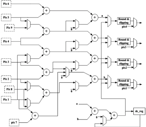
F. Intra-Prediction Generator Unit
Fig. 11 shows the proposed intra-prediction generator unit with the plane mode removal. The whole 13 intra-prediction modes are organized into four types as described in Fig. 3. The modes in these types use the partial sum of adjacent pixels to compute the desired values for different position in a block. To support various computation of intra-prediction, the datapath of this generator can be reconfigured to handle different modes for luma 4 4, luma 16 16, and chroma 8 8.
The operations for all intra-prediction modes are explained in the following. First, the inputs are selected from boundary registers which store the neighboring pixels of previously re-constructed blocks. Then, for the bypass type of vertical and horizontal modes, the prediction generator does nothing but di-rectly outputs the input values. For the linear type, from mode three to mode eight, desired values are obtained by reusing its
partial sums. For example, the first-level adders generate value like , and then the second-level adders sum up the ad-jacent partial sums to compute the results like . As to the average type, so called dc modes, it needs to sum up the eight pixels around the blocks, four upper pixels and four left ones, to figure out the average value. For luma 4 4 or chroma 8 8 dc modes, it takes one cycle to calculate the dc value. However, extra four cycles are required for luma 16 16 dc prediction since up to 32 boundary pixels have to be ac-cumulated. We use extra adders and a register to simplify the accumulation operations in the reconfigurable datapath, which saves more control and wiring circuits. After prediction, these values are handled through the difference unit to produce the residuals, which will be sent to the transform unit for further processing.
G. Transform and Quantization Unit
Though several transform designs have been proposed [7], [8], we adopt the same architecture as in [9] to execute integer transform (DCT) and DHT since it is also four-pixel parallel. In addition, two 4 4 block-size registers are located in both forward and inverse transform units to gather the dc coefficients after transform and inverse transform for further DHT compu-tation of dc blocks.
The quantization and dequantization units are shown in Fig. 12. Constant quantization coefficients are all implemented by look-up tables depending on QP, as denoted by quant_coef, dequant_coef, qp_const, qp_shift, and qp_per in Fig. 12. A quantized value is obtained through a multiplication with quant_coef, an addition of qp_const, and shift. To recover the data, a multiplication followed by rounding and shift is
Fig. 12. Proposed quantization and dequantization units.
performed. The design also uses the data guarding technique to reduce power consumption by skipping the zero inputs.
H. Cost Generation and Mode Decision Unit
After transform, the coefficients are sent to both cost gen-eration unit for cost calculation and current block registers to temporarily be stored. The cost generation is implemented ac-cording to the enhanced SATD function that is divided in two stages: the integer transform that replaces the Hadamard trans-form and the extra scaling factors. The above replacement can eliminate the recomputation issue of transform in hardware de-sign and also improve coding performance. The scaling factors in (9) are realized with a two-stage adder tree and simple shifters instead of multipliers to reduce hardware cost and critical time. The cost is then accumulated for 16 16 prediction or com-pared to the current minimum cost value of 4 4 prediction. If a smaller cost is detected, the minimum cost is replaced by the new one and coefficients in the current block registers are moved to the best block registers. This comparing and replacement pro-cedure will be continued recursively until the best mode with minimum cost is obtained. Eventually, SATD costs of 4 4 prediction and 16 16 prediction are compared again to deter-mine which prediction type is used.
I. Reconstruction Phase
The quantized values are stored in the coefficient buffer for entropy coding, and also need to be reconstructed immediately since prediction unit requires its boundary pixels to predict suc-cessive blocks. Besides, this reconstruction process in the en-coder is the main part of deen-coder as well. The reconstruction phase as shown in Fig. 6 consists of two paths, one for residual reconstruction and one for predictor generation. The residuals are recovered by dequantization, inverse-transform, and scaling shift in the proper order. At the same time, the corresponding predictors are also obtained and added to the residuals for re-construction of data. They are immediately generated by the intra-prediction generator in the decoding process but queued in the reconstruction first-in first-out (FIFO) register in the en-coding process due to the long latency of transform and mode decision process. After reconstruction, some of these data are stored in the boundary buffers as the reference for prediction of next macroblock.
Fig. 13. Proposed architecture for CAVLC encoder.
J. Memory Organization
Only two on-chip memories are used in the proposed codec architecture, a source buffer and a coefficient buffer. The source buffer, a 96-entry 32-bit single-port SRAM, stores four pixels per row, where 64 entries for a luma components and 32 for chroma ones. In the encoding process, this buffer stores the source data of currently encoded macroblock, while in the de-coding process, it can be used to save decoded pixels after recon-struction and then output them to external memory at the end of decoding. The coefficient buffer adopts the ping-pong architec-ture such that the coding loop and entropy coding stage can be pipelined to improve hardware performance. Each bank in the buffer has 104 entries with 64-bit bandwidth for 96 entries of ac coefficients and 8 entries of dc coefficients. Moreover, a line buffer with frame width wide is located in the off-chip memory to store the boundary reference pixels above the current mac-roblock.
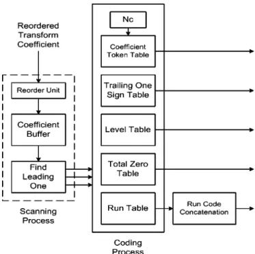
K. CAVLC Codec
Fig. 13 shows the hardware architecture of CAVLC encoder. The encoder can be divided into two parts: scanning process and encoding process, which are work in parallel. During encoding, the transform coefficients are first reordered in the zigzag scan order and then detected and marked as zero if it is zero. The zero coefficients coding is skipped by the leading one detection unit. and only the nonzero ones will be sent to the encoding process. Thus, the corresponding coding data is generated and sent to tables for parallel coding. This efficient zero skipped coding can speedup the process significantly with seven cycles for one block coding in average.
Fig. 14 shows the hardware architecture for CAVLC decoder. This design first decodes the coefficient token and sign mark in the same cycle, and thus the level decoding can be started im-mediately in the next cycle. During the level decoding process,
Fig. 14. Proposed architecture for CAVLC decoder.
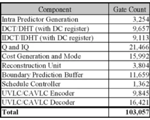
TABLE VIII LIST OFGATECOUNT
the 4 4 zero block information is recorded in the zero block index unit, and the remaining decoding circuit is turned off for such a block. After it, the zero run decoding can be two sym-bols in one cycle if it is less or equal than six, a common case that is worth to be speedup. Once every run is decoded, the de-coded level will be put into their corresponding position in the coefficient buffer, and no extra reordering cycle is required to merge level and zero runs. The cycle count for one macroblock decoding is 90 in average of all sequences when QP is fixed to 28.
V. EXPERIMENTALRESULTS
A. Implementation
The proposed codec IP architecture is designed by Verilog HDL and implemented using the 0.18- m 1P6M CMOS tech-nology. Table VIII lists the gate count for each component, and the total gate count is 103.06 K. In this list, we can observe that the quantization and dequantization unit occupies the largest area since it uses four multipliers in four-pixel parallelism to compute the quantized coefficients. The four-pixel parallel de-sign can provide smooth flow without waiting. Besides, the cost generation and mode decision unit has the second largest area due to the two block-size registers and critical timing in sum-mery. The reconfigurable datapath design and elimination of intra-plane prediction makes our intra-prediction generator only needs 3.3 K gate count.
Fig. 15. Chip layout and specification.
The chip layout is shown in Fig. 15. It has a core size of 1.28 1.28 mm . In this layout, one 96 32-bit SRAM is placed at the top and a pair of dual banks 104 64-bit SRAM is im-plemented at the bottom of the chip. The design can achieve the highest frequency at 125 MHz. Thus, it can easily support 29.62 Mpixels/s still image encoding and real-time video intra-frame coding of high-definition 720p (1280 720 4:2:0 30 fps) video application when clocked at 117 MHz. Besides, it can also support the same decoding throughput with frequency of 25.5 MHz.
B. Comparison With Previous Design
Since no intra-codec has been published, we compare our design with other encoder and decoder design as shown in Table IX. Previous encoder design [4] can only support stan-dard definition (SD) size (720 480 4:2:0 30 fps) at frequency of 54 MHz and has a total gate count of 84 K implemented in TSMC 0.25- m 1P5M CMOS technology. However, it uses two single-port and one dual-port memories in their architecture and results in a larger core size. In addition, it cannot support the decoding process and needs extra area cost for plane prediction. Our design can support both codec and HD size process with slightly larger area and lower operating frequency. The extra area cost is roughly the area cost of CAVLC decoder. The other design [10] is a pure baseline decoder implementation that supports HD 720p size decoding with frequency of 50 MHz. In comparison, our design needs lower operating frequency for the same decoding capability.
TABLE IX DESIGNCOMPARISONS
VI. CONCLUSION
This paper presents an HD 720p MPEG-4 AVC/H.264 intra-codec IP architecture for closed system like digital video recorder and digital still camera. The design uses various techniques to save area cost and enhance throughput. In the algorithm level modification, we adopt the enhanced SATD cost generation function and eliminate the intra-plane prediction to save the area requirement with only small quality loss. In the hardware implementation, the design is pipelined in the mac-roblock level to improve data throughput and scheduled with three techniques to improve hardware utilization and reduce area cost. The decoding process is well included in the design by utilizing the reconstruction path of the encoder loop. The design can support real-time HD 720p size video encoding and decoding at 117 and 25.5 MHz, respectively, and it can support still image encoding at the throughput of 29.62 Mpixels/s at 125 MHz. The implemented chip has total gate count of 103.06 K and a core size of 1.28 1.28 mm .
REFERENCES
[1] Draft ITU-T Recommendation and Final Draft International Standard
of Joint Video Specification, ITU-T Rec. H.264/ISO/IEC 14496-10
AVC, Mar. 2003.
[2] A. Puri, X. Chen, and A. Luthra, “Video coding using the H.264/MPEG-4 AVC compression standard,” Signal Process. Image
Commun., vol. 19, pp. 793–849, 2004.
[3] T. Halbach, “Performance comparison: H.26L intra coding versus JPEG2000,” JVT-D039, Jul. 2002.
[4] Y.-W. Huang, B.-Y. Hsieh, T.-C. Chen, and L.-G. Chen, “Analysis, fast algorithm, and VLSI architecture design for H.264/AVC intraframe coder,” IEEE Trans. Circuits Syst. Video Technol., vol. 15, no. 3, pp. 378–401, Mar. 2005.
[5] H.-M. Wang, C.-H. Tseng, and J.-F. Yang, “Improved and fast algo-rithm for intra 42 4 mode decision in H.264/AVC,” in Proc. IEEE.
Int. Symp. Circuits Syst., May 2005, pp. 2128–2131.
[6] T.-C. Wang, Y.-W. Huang, C.-Y. Tsai, B.-Y. Hsieh, and L.-G. Chen, “Dual-block-pipelined VLSI architecture of entropy coding for H.264/AVC baseline profile,” in Proc. Int. Symp. VLSI Design,
Automat. Test, Apr. 2005, pp. 271–274.
[7] H.-Y. Lin, Y.-C. Chao, C.-H. Chen, B.-D. Liua, and J.-F. Yang, “Combined 2-D transform and quantization architecture for H.264 video coders,” in Proc. IEEE Int. Symp. Circuits Syst., May 2005, pp. 1802–1805.
[8] K.-H. Chen, J.-I. Guo, K.-C Chao, J.-S. Wang, and Y.-S Chu, “A high-performance low power direct 2-D transform coding IP design for MPEG-4 AVC/H.264 with a switching power suppression technique,” in Proc. Int. Symp. VLSI Design, Automat. Test (VLSI-DAT), Apr. 2005, pp. 291–294.
[9] T.-C. Wang, Y.-W. Huang, H.-C. Fang, and L.-G. Chen, “Parallel 42 4 2-D transform and inverse transform architecture for MPEG-4 AVC/H. 264,” in Proc. IEEE Int. Symp. Circuits Syst., May 2003, pp. 800–803. [10] T.-A. Lin, S.-Z. Wang, T.-M. Liu, and C.-Y. Lee, “An H.264/AVC de-coder with 42 4-block level pipeline,” in Proc. IEEE Int. Symp.
Cir-cuits Syst., May 2005, pp. 1810–1813.
Chun-Wei Ku received the B.S. and M.S. degrees in
electronics engineering from National Chiao-Tung University, Hsinchu, Taiwan, R.O.C., in 2004 and 2006, respectively.
After graduation he joined MediaTek, Inc., Hsinchu, Taiwan, R.O.C. His major research inter-ests include H.264/AVC video coding, digital signal processing, and associated VLSI architecture design.
Chao-Chung Cheng received the B.S. and M.S.
degrees in electronics engineering from National Chiao-Tung University, Hsinchu, Taiwan, R.O.C., in 2003, and 2005, respectively. He is currently working toward the Ph.D. degree in the Graduate Institute of Electronics Engineering from National Taiwan University, Taiwan, R.O.C.
His research interests include digital signal pro-cessing, video system design, and computer architec-ture.
Guo-Shiuan Yu received the B.S. and M.S. degrees
in electronics engineering from National Chiao-Tung University, Hsinchu, Taiwan, R.O.C., in 2004 and 2006, respectively.
He is currently with Faraday Technology, Inc., Hsinchu, Taiwan, R.O.C.. His research interests include multimedia video system and digital signal processing.
Min-Chi Tsai received the B.S. and M.S. degrees in
electronics engineering from National Chiao-Tung University, Hsinchu, Taiwan, R.O.C., in 2004 and 2006, respectively.
He is currently with Andes Technology, Inc., Hsinchu, Taiwan, R.O.C. His research interests include VLSI design, digital IC design, and memory management for multimedia platform SoC.
Tian-Sheuan Chang (S’93–M’06) received the
B.S., M.S., and Ph.D. degrees in electronics en-gineering from National Chiao-Tung University, Hsinchu, Taiwan, R.O.C., in 1993, 1995, and 1999, respectively.
He is currently with Department of Electronics Engineering, National Chiao-Tung University, as an Assistant Professor. During 2000–2004, he worked at Global Unichip Corporation, Hsinchu, Taiwan, R.O.C. His research interests include IP and SOC design, VLSI signal processing, and computer architecture.