無線區域網路中以位置認知及使用者習性為基礎的遞交演算法

全文

(1)國立交通大學電信工程學系碩士論文. 無線區域網路中以位置認知及使用者習性為基礎的遞交演算法 Location-Aware and Profile-Based Handoff in WLAN. 研究生︰廖怡翔指導教授：廖維國博士. 中華民國九十三年十月.

(2) 無線區域網路中以位置認知及使用者習性為基礎的遞交演算法 Location-Aware and Profile-Based Handoff in WLAN 研究生︰廖怡翔指導教授︰廖維國博士. Student: Yi-Hsiang Liao Advisor: Dr. Wei-Kuo Liao. 國立交通大學電信工程學系碩士論文. A Thesis Submitted to the Department of Communication Engineering College of Electrical Engineering and Computer Science National Chiao Tung University in Partial Fulfillment of the Requirements for the Degree of Master of Science In Communication Engineering Oct 2004 Hsinchu, Taiwan, Republic of China 中華民國九十三年十月.

(3) Chinese Abstract. 無線區域網路中以位置認知及使用者習性為基礎的遞交演算法研究生︰廖怡翔. 指導教授︰廖維國博士. 國立交通大學電信工程學系碩士班. 中文摘要隨著 WLAN 以及 VOIP 技術的成熟，以及雙網整合的實現，在未來，WLAN 中的 AP 將會扮演行動通訊中的基地台的角色。因此，WLAN 中的遞交將成為一個重要的課題。遞交演算法的優劣，不只影響通話品質，也會影響頻道的使用效率。在行動通訊中，信號的強度對通訊的品質有直接與立即的影響。因此，利用接收信號的強度（RSS）來作為判斷是否遞交(handoff)到新的基地台的條件，似乎是既合理又簡單的方法。在無死角無阻礙的開放空間中，這種方法的確沒有問題。但在 WLAN 的環境下，由於信號除了受到雜訊干擾外，亦受到多重路徑干擾(multi-path reflecting)的影響，使得信號的強度極有可能在相鄰的區域亦會相差甚遠，因而使得正在傳輸中的行動基地台將信號切換到鄰近信號較佳的基地台上。但是由於信號可能只是暫時地減弱，若是遞交過去的基地台也只是一時信號較佳，將造成強迫斷訊(forced terminated)或多餘的遞交。本篇論文即是以通話品質(call quality)作為決定遞交依據的方法。並利用使用者習慣路徑和信號強度表兩種方法，來修正以在無線區域網路通話品質作為遞交依據的缺點。.

(4) Location-Aware and Profile-Based Handoff in WLAN English Abstract Student: Yi-Hsiang Liao. Advisor: Dr. Wei-Kuo Liao. Department of Communication Engineering National Chiao Tung University. Abstract With the growth of WLAN and VOIP, access points (AP) in WLAN will play the role of base station in cellular system in the future. As the reason, handoff algorithm in WLAN will be an important issue in the future. The performance of handoff algorithms effect not only call quality, but also the spectral efficiency. In mobile communication, signal strength has immediate effect on communication quality. As the reason, it’s reasonable to use received signal strength (RSS) as the matrix of deciding handoff. This method performs well in an open space. However, due to the severe effect of multi-path fading in WLAN, signal strength changes rapidly in close distance probably. This effect may cause unnecessary handoffs and service failures (forced termination), which both influence call quality. In this thesis, we use call quality criterion as handoff algorithm. We propose location-aware and profile-based methods to tackle problems signal strength prediction in WLAN.. ii.

(5) 誌謝感謝所有對我這兩年來照顧的師長朋友們，尤其是感謝我的指導教授廖維國老師兩年來對我的日常生活教誨與研究態度培養，使我在這兩年中學到了作任何事都必需具備的細心與嚴謹態度。也感謝我親愛家人與好友在這兩年對我的支持，你們是我向上提升的原動力。也感謝實驗室學長們在我困惑時給予的指導，幫助我解決問題及找到方向，使我的論文可以順利完成。還有可愛的同學以及學弟們，政澤、怡中、國瑋、柏谷、賢宗、健智、憲良、于彰，謝謝你們陪我度過快樂的時光。在此僅向所有關心我的人致謝，謝謝你們對我的支持鼓勵。. Acknowledgment. iii.

(6) Contents Chinese Abstract ........................................................................................................................ 1 English Abstract ......................................................................................................................... ii Acknowledgment....................................................................................................................... iii Contents ..................................................................................................................................... iv List of Tables............................................................................................................................... 1 List of Figures............................................................................................................................. 1 Introduction................................................................................................................................ 2 Related Background .................................................................................................................. 4 2.1 DARAR System............................................................................................................. 4 2.1.1 Introduction......................................................................................................... 4 2.1.2 Off-line Reference Data Collection – Empirical Method ................................... 5 2.2 Dynamic Programming Algorithm ................................................................................ 6 2.2.1 Bellman Equation................................................................................................ 6 2.2.2 Dynamic Programming Algorithm ..................................................................... 7 2.2.3 Dynamic Programming in Handoff Problem ...................................................... 7 2.3 Locally Optimal Handoff Algorithm ............................................................................11 Handoff Algorithms ................................................................................................................. 12 3.1 User Profile .................................................................................................................. 12 3.2 Table Lookup ............................................................................................................... 14 3.3 DP Solution .................................................................................................................. 14 Simulation................................................................................................................................. 19 4.1 Building Layout ........................................................................................................... 19 4.2 Data Collection ............................................................................................................ 21 4.2.1 RADAR’s Database .......................................................................................... 21 4.2.2 User Profile ....................................................................................................... 22 4.3 Simulation.................................................................................................................... 22 4.4 Numerical Result ......................................................................................................... 26 Conclusion ................................................................................................................................ 29 Reference .................................................................................................................................. 30. iv.

(7) List of Tables Table 4-1 Simulation result of DP process (1)…………………….…………………………23 Table 4-2 Simulation result of DP process (2)………………………………………………24 Table 4-3 Simulation result of DP process (3)…..……….…………………………………25 Table 4-4 Simulation result of DP process (4)………………………………………………25. List of Figures Fig. 2-1 Triangulation…………………………………………………………………….…5 Fig. 4-1 Placement of BS on floor 7…………………….…..………………………………19 Fig. 4-2 Placement of BS on floor 8……………….….……………………………………20 Fig. 4-3 Placement of BS on floor 9……………………..…………………………………20 Fig. 4-4 Number of base stations at chose locations……………………..…………………21 Fig. 4-5 The number of handoff versus c (tradeoff parameter)…………………………….26 Fig. 4-6 The number of service failure versus c (tradeoff parameter)………….…………..27 Fig. 4-7 Bayes formula (c*handoff number + service failure number) versus c (tradeoff parameter)………..………………………………….…………………………...28.

(8) Chapter 1 Introduction. Voice over IP in Wireless LAN (WLAN) is seen as one of the most important services for telecommunication providers. To guarantee the quality of such service, the seamless handoff, i.e., transferring an ongoing association with one access point to another as a user moves through the boundary of coverage of access point without user’s perception, therefore becomes a necessary requirement. In this thesis, we study the decision of when to perform a handoff for such a service. In close examination, two considerations are needed to be taken in designing the handoff decision algorithm. The first is the spectral efficiency, i.e. the maximum number of connections the system can serve in an area. A better algorithm needs fewer channels preserved for handoff because it has less unnecessary handoffs [5]. Second, the handoff decision also influences the quality perceived by users. When the drop in measured signal strength is due to momentary fading, a call may be handed off back and forth between neighboring base stations, or is forced to terminate as the signal strength below the acceptable level if without proper handoff. Thus, a good handoff decision algorithm must reduce the chance of not only the unnecessary handoffs but also the forced termination. Several metrics, such as received signal strength (RSS), signal to interference ratio (SIR), distance, transmit power, traffic load, and mobile velocity, are used in traditional handoff decision algorithms dedicated to cellular systems. However, in our experiments the traditional handoff decision algorithms based on stochastic and heuristic models perform poorly in WLAN environment. Two major causes of the problem are highly location-dependent radio signaling in WLAN environment due to serious multipath fading [8] and non-stationary user’s motion process [9]. In our design, to tackle the first cause of problem, we use location-aware approach to assist the signaling prediction. That is, the system identifies the user’s location first and then queries the database to predict signal strength. The problem of non-stationary user’s motion process is handled by using the user’s profile to track down the user’s motion. We then use 2.

(9) the dynamic programming technique to accommodate the obtained information for handoff decision making. We perform an empirical study on our proposed algorithm. With the full probabilistic description of user’s motion process and a viable geolocation technology in WLAN environment called RADAR [1], our proposed algorithm outperforms the traditional algorithms. RADAR system and dynamic programming principles will be briefly introduced in Chapter 2. Our proposed solution based on dynamic programming will be introduced in Chapter 3. In Chapter 4, we will present our experiment result. We draw the conclusion in Chapter 5.. 3.

(10) Chapter 2 Related Background. 2.1 DARAR System Among indoor location systems, Radio frequency (RF) networks offer a significant advantage over IR networks in terms of range, scalability, deployment, and maintenance. Thus we use RADAR as our location system. 2.1.1 Introduction RADAR is a radio-frequency (RF) based system for locating and tracking users inside buildings. RADAR records and processes signal strength information at multiple base stations positioned to provide overlapping coverage in the area of interest. It combines empirical measurements with signal propagation modeling to determine user location. The basic approach of RADAR is triangulation. Given a set of signal strength measurements at each of the base stations, we determine the location that best matches the observed signal strength data. We then “guess” that to be the location of the user. The number of signal strength set must not less than three. Suppose each mobile device can detect three signal strengths from three bass stations in wireless LAN environment. Three circumferences refer to a certain set of SS at three base stations at the points of circumferences. As we can see in Fig. 1, a set of two signal strengths determines two points, but three signal strengths set can decide only one point, that what’s the purpose of a location system.. 4.

(11) Fig. 2-1 Triangulation RADAR terms its general technique nearest neighbor(s) in signal space (NNSS). The idea is to compute the distance (in signal space) between the observed set of SS measurements, (ss1, ss2, ss3), and the recorded set of SS, (ss’1, ss’2, ss’3), at a fixed set of locations. Then we pick the location that minimizes the Euclidean distance, i.e., sqrt((ss1 – ss’1)2 + (ss2 – ss’2)2 + (ss3 – ss’3)2).. 2.1.2 Off-line Reference Data Collection – Empirical Method In data collecting process, there are two methods: empirical method and propagation model method. We choose the former for our experiment. Due to the fact that signal strength at a given location varies quite significantly (by up to 5dBm) depending on the user’s orientation. So, in addition to user’s location, we also recorded the direction of the user (one of north, south, east, or west) when the measurement is made. In the empirical method, we collect at least 20 signal strength samples at each reference point in 4 directions. Thus at least 20*4=80 samples must measured at each reference point. Combining these samples with the location and orientation, we define a SS tuple, (x, y, d, ss1, ss2, ss3), where x and y are coordinate of position, d is the direction, ssi is the signal strength of ith base station. For each (x, y, d) tuple, calculate the mean, the standard deviation, and the median of the samples of each direction of each reference point.. 5.

(12) 2.2 Dynamic Programming Algorithm Dynamic programming deals with situations where decisions are made in stages. The outcome of each decision may not be fully predictable but can be anticipated to some extent before the next. The objective is to minimize a certain cost – a mathematical expression of what is considered an undesirable outcome. The key aspect of such situations is that one must take the tradeoff between the desire of low present cost and undesired high future costs. Therefore, at each stage, decisions are made based on the sum of present cost and the expected future cost.. 2.2.1 Bellman Equation The basic model of dynamic programming systems has two features: (1) an underlying discrete-time dynamic system, and (2) a cost function that is additive over time. The dynamic system expresses the evolution of some variables, the system “state”, under the influence of decisions made at discrete instance of time. The system has the form x k +1 = f k ( x k , u k , wk ), k = 0,1,K , N − 1 where k indexes discrete time, x k is the state of the system and summarizes past information that is relevant for future optimization, u k is the control or decision variable to be selected at time k , wk is a random parameter (also called disturbance or noise), N is the number of times control is applied, f k is a function that describe the system and the mechanism by which the state is update.. The cost function is additive in the sense that the cost incurred at time k, denoted by g k ( x k , u k , wk ) , accumulates over time. The total cost is N −1. g N ( x N ) + ∑ g k ( x k , u k , wk ) k =0. where g N ( x N ) is a terminal cost incurred at the end of the process. However, because of the presence of wk , the cost is generally a random variable and cannot be meaningfully optimized. We therefore formulate the problem as an optimization of the expected cost N −1 ⎫ ⎧ E ⎨ g N ( x N ) + ∑ g k ( x k , u k , wk )⎬ k =0 ⎭ ⎩ where the expectation is with respect to the joint distribution of the random variables involved. The optimization is over the controls, but each control u k is selected with some. 6.

(13) knowledge of the current state x k .. 2.2.2 Dynamic Programming Algorithm The dynamic programming (DP) technique base on a simple idea, the principle of optimality. Roughly, the principle of optimality states the following obvious facts. Principle of Optimality Let π ∗ = µ 0∗ , µ1∗ ,K, µ N∗ −1 be an optimal policy for the basic problem, and assume. {. }. that when using π , a given state xi occurs at time i with positive probability. Consider the subproblem whereby we are at xi at time i and wish to minimize the “cost-to-go” from time i to time N ∗. N −1 ⎧ ⎫ E ⎨ g N ( x N ) + ∑ g k ( x k , u k , wk )⎬ k =i ⎩ ⎭. {. }. Then the truncated policy µ i∗ , µ i∗+1 ,K, µ N∗ −1 is optimal for this subproblem.. The principle of optimality suggests that an optimal policy can be constructed in the following steps. First construct an optimal policy for the “tail subproblem” involving the last stage. Then extend the optimal policy to the “tail subproblem” involving the last two stages. Continue in this manner until an optimal policy for the entire problem is constructed.. 2.2.3 Dynamic Programming in Handoff Problem In [3], a dynamic programming algorithm in handoff is proposed. Dynamic programming allows optimization of the total cost along a state trajectory of a discrete-time dynamical system that has a stepwise additive-cost criterion and, conditioned on the state, stepwise independent-noise statistics. First, the signal strength X k(i ) received from base station Bk(i ) at distance d k(i ) at kth sampling instant can be written as. ( ). X k(i ) d (i ) = µ − η log d k(i ) + Z k(i ) dB. i = 1, 2. where μ and η account for path loss, μ depends on the transmitted power at the base 7.

(14) station, and η is the path-loss exponent. The term Z k(i ) is the shadow fading component, which is accurately modeled (in decibels) as a zero-mean stationary Gaussian random process [14] Suppose there are total of n time steps k = 1, 2, …, n on the portion of the mobile’s trajectory that involves B (1) and B (2 ) . Let Bk denote the index of the operative base station at time k (i.e., Bk = i when the mobile is communicating with B(i)) and Bkc denote the other AP. A handoff decision is made during each sampling interval. The decision variable U k that takes on two values can be based in all signal strength measurements up to time k. If U k = 1, a handoff is made resulting in Bk+1 = Bkc . If U k = 0, no handoff is made and Bk+1= Bk+1. Handoff algorithm design involves choosing the handoff decision function φ k at times. k = 1, 2, …, n-1. Let ∆ denote the minimum level of signal strength required for satisfactory service. And let NSF and NH denote the total number of service failures and number of handoffs from time 1 to n. Then. {. ⎡ n E[N SF ] = E ⎢∑ Ι X k( Bk ) < ∆ ⎣ k =1. }⎤⎥ = ∑ Pr{X ( n. ⎦. k =1. Bk ). k. <∆. }. ⎤ n −1 ⎡ n −1 E[N H ] = E ⎢∑ Ι{U k = 1}⎥ = ∑ Pr{U k = 1} ⎦ k =1 ⎣ k =1. where I{‧} is the indicator function. An optimal handoff algorithm is the set of decision function φ which provides the best tradeoff between the E[NSF] and E[NH]. This optimal tradeoff problem can be posed in Bayes formulation: min cE[N H ] + E[N SF ] φ. where c > 0 is a tradeoff parameter.. (. ). For the handoff problem, the state S k at time k consists of X k(1) , X k(2 ) , Bk , where Bk denotes the base station which mobile communicates with at time. Thus we get the following update equation for S k :. 8.

(15) ⎡ X k(1+)1 ⎤ ⎢ ⎥ S k +1 = ⎢ X k(2+)1 ⎥ = f (S k ,U k , Wk ) ⎢ Bk +1 ⎥ ⎣ ⎦ (1) ⎡ X k − η log d k(1+)1 + η log d k(1) + Wk(1) ⎤ ⎢ ⎥ = ⎢ X k(2 ) − η log d k(2+)1 + η log d k(2 ) + Wk(2 ) ⎥ ⎢ ⎥ Bk Ι{U k = 0} + Bkc Ι{U k = 1} ⎣ ⎦. [. ]. where Wk(i ) = Z k(i+1) − Z k(i ) is the change in the fading process and Wk = Wk(1) ,Wk(2 ) . The update function f (S k , U k , Wk ) constitutes a discrete-time dynamical model for the system.. { }. { }. Given the first-order AR model for process Z k(1) and Z k(2 ) , the noise variables Wk have the required independence structure. Finally, the cost criterion as defined before is additive over time. If we define. {. }. g k (S k ,U k ) = cΙ{U k = 1} + Ι X k( Bk ) < ∆ ,. {. 1 ≦ k ≦ n-1,. }. g n (S n ) = Ι X n( Bn ) < ∆ . then, the Bayes optimal handoff algorithm minimizes n −1. E[g n (S n )] + ∑ E[g k (S k , U k )] k =1. The DP solution is obtained recursively as follows. Let the expected cost-to-go of base station Bk at time k (due to all the decisions up to time k) be denoted by J k( Bk ) . Then the optimal handoff decision functions are obtained by solving the follow set of recursive equatins:. (. {. ). J n X n(1) , X n(2 ) , Bn = g n (S n ) = Ι X n( Bn ) < ∆. (. J n −1 X n(1−)1 , X n(2−)1 , Bn −1. ). [ ) < ∆}+ min [Pr {X (. }. (. = min EWn−1 S n−1 g n −1 (S n −1 ,U n −1 ) + J n X n(1) , X n(2 ) , Bn φ n −1. {. = Ι X n( B−1n−1. n. B n −1 ). }. )]. {. < ∆ X n( B−1n−1 ) , c + Pr X n(Bn−1 ) < ∆ X n(B−n1−1 ). and for k = n-2, n-3, …, 1 9. c. c. }].

(16) (. J k X k(1) , X k(2 ) , Bk. [. ). (. = min EWk S k g k (S k , U k ) + J k +1 X k(1+)1 , X k(2+)1 , Bk +1 φk. {. ( Bk ). = Ι Xk. { ( { (. )]. } }. ) ). ⎛ E J k +1 X k(1+)1 , X k(2+)1 , Bk +1 X k(1) , X k(2 ) , ⎞ ⎟ < ∆ + min⎜⎜ c ( 1 ) ( 2 ) ( 1 ) ( 2 ) ⎜ E J k +1 X k +1 , X k +1 , Bk +1 X k , X k + c ⎟⎟ ⎠ ⎝. }. For each k, the optimum decision function φ k* depends only on the state Sk and not on any past signal-strength measurements. These optimum decision functions are described by. { = 0 : if Pr {X (. } { ) }< c + Pr{X (. } )}. U n −1 = 1 : if Pr X n( Bn −1 ) < ∆ X n( B−1n −1 ) > c + Pr X n(Bn −1 ) < ∆ X n(B−1n −1 ) U n −1. n. Bn −1 ). < ∆ X n( B−1n −1. c. Bnc −1 n. c. ) < ∆ X (B. c n −1. n −1. (1). and for k = 1, 2, …, n-2. { ( } { ( } ) ) . = 0 : if E{J (X ( ) , X ( ) , B ) X ( ) , X ( ) } < c + E{J (X ( ) , X ( ) , B ) X ( ) , X ( ) }. U k = 1 : if E J k +1 X k(1+)1 , X k(2+)1 , Bk +1 X k(1) , X k(2 ) > c + E J k +1 X k(1+)1 , X k(2+)1 , Bkc+1 X k(1) , X k(2 ) Uk. k +1. 1 k +1. 2 k +1. k +1. 1 k. 2. k +1. k. 1 k +1. 2 k +1. c k +1. 1 k. 2. k. For the lognormal fading model that we have assumed, the conditional distribution of X k(i+)1 given X k(i ) is Gaussian, hence the probabilities in (1) are entirely determined by the conditional means and variances ⎡ d (i ) ⎤ E X k(i+)1 I k = aX k(i ) + (1 + a )µ log ⎢ k +1 a ⎥ ⎢⎣ d k(i+)1 ⎥⎦. [. ]. [. ( ). ] (. ). Var X k(i+)1 I k = 1 − a 2 σ 2 ,. where a is the correlation coefficient of the discrete-time fading process.. 10.

(17) However, with d k(i ) and d k(i+)1 unknown, we are forced to use the best available estimate. [. ]. of E X k(i+)1 I k , denoted as Xˆ k(i+)1 , base on the available information I k . The resulting decision function are: U n −1. U n −1. c ⎡ ∆ - Xˆ k(B+k1 ) ⎡ ∆ - Xˆ k( B+1k ) ⎤ = 1 : if Q ⎢ ⎥ > c + Q⎢ 2 ⎢⎣ σ 1 − a 2 ⎣⎢ σ 1 − a ⎥⎦. ⎤ ⎥ ⎥⎦. c ⎡ ∆ - Xˆ k(B+k1 ) ⎤ ⎡ ∆ - Xˆ k( B+1k ) ⎤ = 0 : if PQ ⎢ ⎥ ⎥ < c + Q⎢ 2 2 ⎣⎢σ 1 − a ⎥⎦ ⎣⎢σ 1 − a ⎥⎦. where Q( x ) =. ∞. ⎛ − x2 ⎞ exp ∫ ⎜⎜⎝ 2 ⎟⎟⎠dx . 2π x 1. 2.3 Locally Optimal Handoff Algorithm Locally optimal handoff algorithm is a special case of dynamic programming algorithm. It predicts only one step future to determine handoff [3]. In cellular system, the prediction of signal strength performs well because of smooth fading of signal strength and stationary user’s motion. However, such estimation of signal strength is not adequate for WLAN because the signal strength is highly location-dependent in WLAN. Thus signal strength may fluctuate severely in adjacent place in an indoor environment. This causes the prediction of signal strength based on signaling history very poor in WLAN. Severe fluctuation of signal strength also indicates that locally optimal algorithm is not enough to make proper decision. One-step prediction of signal strength indicates short trend of signal strength, but depending only on this prediction may cause unnecessary handoff because the fluctuation of signal strength. Additionally, the tradeoff parameter c in locally optimal algorithm can not large than one. It’s not reasonable in Bayes formula. In next chapter, our proposed method, user profile and table lookup, can tackle these problem of prediction of signal strength. Then we accommodate this predicted information to dynamic programming to make handoff decisions.. 11.

(18) Chapter 3 Handoff Algorithms. To use DP algorithm for deciding handoff, we must predict signal strength in several future steps. Our approach contains three steps to predict signal strength according to measured signal strength. First, we use RADAR to locate mobile user. If there is only one RSS can be detected, RADAR can’t locate mobile user. However, the mobile user doesn’t need deciding handoff, either. Second, we use this location information and estimated direction to look up user profile for next location and direction. Third, we look up the predicted location in the database of RADAR, which contains location and signal strength information, to predict signal strength. After signal strength predicted, we apply dynamic programming approach to make optimal handoff decisions. The RADAR location system has explained in Chapter 2. In the following section, we will explain the part of user profile, table lookup, and DP solution for WLAN.. 3.1 User Profile We know that the motion of the mobile user in a building is quasi-stationary. Thus we can’t predict the user’s location by its motion history. We use RADAR system to locate mobile user when it detect two or more RSSs from different base stations. As the mobile user moves into the overlapping area of the coverage of two or more base stations, it involves in deciding handoff or not. If there is only one RSS can be detected, RADAR can’t locate mobile user. However, the mobile user doesn’t need deciding handoff, either. Because the number of base stations are more than three, i.e. user will detect different base station in different locations, we have to record the ID of base station that we have measured. Thus we have a new form of the record tuple:. (x, y, n. BS. , BS1 , BS 2 , BS 3 , R 1 ,V 1 , R 2 ,V 2 , R 3 ,V 3 , R 4 , V 4. ). where nBS is the number of base stations mobile user can detect, which maximum is 3, and BSi (i = 1, 2, 3) is the ID of base stations that can be detected, and 12.

(19) (R ,V ) = (rss , rss i. i. i. i. 1. 2. , rss i3 , var1i , var2i , var3i. ). where R and V are mean and variation of each base station and the superscript i denote the direction and the subscript discriminates different base stations. As time goes by, we keep last five location histories to estimate the mobile user’s velocity (speed and direction). According to the present location and velocity, we look up another table, user profile, to find next location. User profile is constructed for each different mobile user, i.e. every mobile user has its own user profile. The user profile for one particular mobile user is constructed by recording its location. The tuple of user profile has the form: (x, y, D1 , D2 , D3 , D4 ). (. ). where Di = xi1 , y i1 , d i1 , Pi1 , xi2 , y i2 , d i2 , Pi 2 , xi3 , y i3 , d i3 , Pi 3 , xi4 , y i4 , d i4 , Pi 4 . (x,y) denotes the. (. ). present estimated location. xij , y ij is the next location on the direction j with probability Pi j given the present estimated location (x,y) and direction i of mobile user when estimated speed is not equal to zero .(If the estimated speed is zero, the predicted location is trivially the current location). d i j is the next direction after location transition. If any one probability of the four directions in Di (i = 1, 2, 3, 4), say P1, is much larger than others, we can reduce Di to. (x , y , d 1 i. 1 i. 1 i. ). , Pi1 , the most probable next location given the present direction i. Thus the tuple. of user profile can be simplified as follow:. (x, y, x1 , y1 , d1 , x 2 , y 2 , d 2 , x3 , y3 , d 3 , x4 , y 4 d 4 ) where (xi,yi) is the predicted location given the present location (x,y) and estimated direction i, and di is the next direction of mobile user on (xi,yi). When the estimated speed is not zero, the predicted location Lk+1 and direction dk+1 based on the information of current estimated location Lk and direction dk can be represented as profile function :. (Lk +1 , d k +1 ) = ψ (Lk , d k ) 13.

(20) 3.2 Table Lookup We know the received signal strength is highly dependent on the structure of the building, thus we can’t predict the mobile user’s signal strength by signal history. After we find its most probable location in next sample time by user profile, we can use this location to “table lookup” associating RSS information. An of-the-shelf table is the database of RADAR system, which contains many locations and its related means and variances of RSS in four directions (north, east, west, south). The signal strength tuple at (k+1) sampling time which result from table lookup can be represent as a table lookup function:. (n. BS , k +1. , BS (1),k +1 , BS (2 ),k +1 , BS (3 ),k +1 , rss (d1k),+k1 +1 , rss (d2k)+,1k +1 , rss (d3k)+,k1 +1 , var(1d)k,+k1+1 , var(d2k),+k1+1 , var(d3)k,+k1+1. = ζ (Lk +1 , d k +1 ). ). After we collect n RSS data, i.e. we predict the RSS in the future n sample times from now on, we can calculate these data by dynamic programming algorithm.. 3.3 DP Solution In locating process by using RADAR, the location of mobile user is function of signal strength. Thus we can represent location variable Lk as:. (. Lk = ( x k , y k ) = l X k(1) , X k(2 ) , X k(3 ). ). By motion history of user, we estimated the velocity of user. Then use current location and velocity of user, we consult the user profile to predicted next location and direction: (Lk +1 , d k +1 ) = ψ (Lk , d k ) Then we use RADAR’s database to look up number of base stations, base stations ID, mean and variance of signal strength received from these base stations. This is done by table lookup function:. (n. BS ,k +1. ). , BS(1),k +1 , BS(2 ),k +1 , BS(3 ),k +1 , rss(d1k),+k1 +1 , rss(d2k)+,1k +1 , rss(d3k)+,1k +1 , var(1d)k,+k1+1 , var(d2k),+k1 +1 , var(d3k),+k1+1 = ζ (Lk +1 , d k +1 ). After predicting n locations and RSS information in the future n sampling instants, we can start to perform DP solution. 14.

(21) As in Chapter 3, we need to calculate Bayes optimal handoff cost: n −1. E[g n (S n )] + ∑ E[g k (S k , U k )] k =1. The DP solution is obtained recursively as follows. Let the expected cost-to-go of base station Bk at time k (due to all the decisions up to time k) be denoted by J k( Bk ) . Then the optimal handoff decision functions are obtained by solving the follow set of recursive equations:. (. {. ). J n( Bn ) X n(1) , X n(2 ) , X n(3 ) , Bn = J n( Bn ) (S n ) = Ι X n( Bn ) < ∆. (. J n( B−1n −1 ) X n(1−)1 , X n(2−1) , X n(3−)1 , Bn −1. [. ). }. ]. = min EWn −1 |S n −1 J n( Bn ) (S n ) + g n −1 (S n −1 , U n −1 ) φ n −1. {. {. = Ι X n( B−1n −1 ). }. ⎡Pr X n( Bn −1 ) < ∆ Ln −1, d n −1 , ⎤ ⎢ ⎥ (B cn1−1 ) ⎢ < ∆ + min Pr X n < ∆ Ln −1, d n −1 + c,⎥ ⎢ ⎥ ⎢Pr X (B cn2−1 ) < ∆ L d + c ⎥ n n −1, n −1 ⎣ ⎦. { {. }. } }. (2). and for k = n – 2, n – 3, … , 1. (. J k( Bk ) X k(1) , X k(2 ) , X k(3 ) , Bk = min EWk φk. {. = Ι X k( Bk ). Sk. [J. ( Bk + 1 ). k +1. (X. (1). k +1. ⎡E ⎢ < ∆ + min ⎢ E ⎢ ⎢E ⎣. }. ). ]. ). , X k(2+)1 , X k(3+)1 , Bk +1 + g k (S k , U k ). {J ( ) (X ( ) , X ( ) , X ( ) , B ) L , d }, ⎤ ⎥ {J ( ) (X ( ) , X ( ) , X ( ) , B ) L , d }+ c,⎥⎥ {J ( ) (X ( ) , X ( ) , X ( ) , B ) L , d }+ c ⎥⎦ Bk k +1. 1 k +1. 2 k +1. 3 k +1. k +1. k. k. B ck1. k +1. 1 k +1. 2 k +1. 3 k +1. k +1. k. k. B ck 2 k +1. 1 k +1. 2 k +1. 3 k +1. k +1. k. k. where the superscripts c1 and c2 of B denote the other two base station that the mobile can detect. At last, we must find. [{. } {. }. {. {. }. } ]. c1 c2 J 0 (S 0 ) = min E J1( B0 ) (S1 ) , E J1(B0 )(S1 ) + c, E J1(B0 )(S1 ) + c. φ0. where B0 denote the communicating base station. Thus our decision function is: If J 0 (S0 ) = E J1( B0 ) (S1 ) , no handoff is made. If 15.

(22) {. }. {. }. c1 c2 J 0 (S0 ) = E J1(B0 )(S1 ) + c , mobile user handoff to B0c1 . If J 0 (S 0 ) = E J1(B0 )(S1 ) + c , mobile. user handoff to B0c 2 .. The signal strength X k( B+1k ) received from base station Bk +1 given location Lk and direction d k at (k+1)th sampling instant can be model as: X k( B+1k +1 ) = h(ζ (Lk +1 , d k +1 ), Bk +1 ) + Wk +1. = h(ζ (ψ (Lk , d k )), Bk +1 ) + n(ζ (Lk +1 , d k +1 ), Bk +1 ). = h(ζ (ψ (Lk , d k )), Bk +1 ) + n(ζ (ψ (Lk , d k )), Bk +1 ). where Wk models the randomness of signal, h denotes the function of table lookup of mean of signal strength, and n denotes the function of table lookup of variance of signal strength. We assume the distribution of signal strength is Gaussian (in decibels)[14]. The model is referred to as the lognormal fading model. Thus the probabilities in (2) are entirely determined by the conditional mean and variances. [. ]. E X k( B+1k +1 ) Lk , d k = h(ζ (Lk +1 , d k +1 ), Bk +1 ) = h(ζ (ψ (Lk , d k )), Bk +1 ). [. ]. Var X k( B+1k +1 ) Lk , d k = n(ζ (Lk +1 , d k +1 ), Bk +1 ) = n(ζ (ψ (Lk , d k )), Bk +1 ) .. Thus ⎡ ∆ − h(ζ (ψ (Lk , d k )), Bk +1 ) ⎤ Pr X k( B+1k +1 ) < ∆ Lk , d k = Q ⎢ ⎥ ⎣⎢ n(ζ (ψ (Lk , d k )), Bk +1 ) ⎦⎥. {. where Q( x ) =. }. ∞. ⎛ − x2 ⎞ exp ∫ ⎜⎜⎝ 2 ⎟⎟⎠dx . 2π x 1. 16.

(23) To explain our DP solution process, we give an example of n = 3. We assume the communicating base B0 = 1, and cost = 0.5. Pb 1. Jk J3 J2 J1. Pb 2 0.9 0.6 0.3. Pb 3 0.7 0.3 0.1. J1 0.1 0.2 0.2. J2 0.9 1.2 1.1. J3 0.7 0.9 0.9. 0.1 0.3 0.5. Let’s define J i j as the element both on line J j and row J i and Pbi j is the element. (. ). both on the line Pb j and row J i . J i j is the expected value of J i j X i(1) , X i(2 ) , X i(3 ) , j . Pbi j is calculated by Q function explained before. At first we calculate J 3j , which is exactly the probabilities Pb3j . Then to calculate J 2j ,. [ (. )]. J 21 = E J 21 X 2(1) , X 2(2 ) , X 2(3 ) ,1. (. = Pb21 + min J 31 , J 32 + c, J 33 + c. ). = 0.6 + min(0.9, 0.7 + 0.5, 0.1 + 0.5) = 1.2. [ (. J 22 = E J 22 X 2(1) , X 2(2 ) , X 2(3) ,2. (. )]. ). = Pb22 + min J 31 + c, J 32 , J 33 + c. = 0.3 + min(0.9 + 0.5, 0.7, 0.1 + 0.5) = 0.9. [ (. J 23 = E J 23 X 2(1) , X 2(2 ) , X 2(3 ) ,3. (. )]. = Pb23 + min J 31 + c, J 32 + c, J 33. ). = 0.2 + min (0.9 + 0.5, 0.7 + 0.5, 0.1) = 0.3. Then to calculate J 1j ,. [ (. )]. J 11 = E J 11 X 1(1) , X 1(2 ) , X 1(3 ) ,1. (. = Pb + min J , J + c, J 23 + c 1 1. 1 2. 2 2. ). = 0.3 + min(1.2, 0.9 + 0.5, 0.3 + 0.5) = 1.1. [ (. J 12 = E J 12 X 1(1) , X 1(2 ) , X 1(3 ) ,2. (. )]. = Pb + min J + c, J , J 23 + c 2 1. 1 2. 2 2. ). = 0.1 + min (1.2 + 0.5, 0.9, 0.3 + 0.5) = 0.9. 17. ..

(24) [ (. J 13 = E J 13 X 1(1) , X 1(2 ) , X 1(3 ) ,3. (. )]. = Pb13 + min J 21 + c, J 22 + c, J 23. ). = 0.2 + min (1.2 + 0.5, 0.9 + 0.5, 0.3) = 0.5. At last step, because communicating B0 is 1,. [. J 0 = min J 11 , J 12 + c, J 13 + c. ]. = min[1.1,0.9 + 0.5,0.5 + 0.5] = 0 .5 + 0 .5 = J 13 + c. Because the expected cost of transferring to B0c = 3 is smaller than remaining on B0 = 1 , the system decides to make a handoff to B0c = 3 .. 18.

(25) Chapter 4 Simulation. 4.1 Building Layout Our WLAN environment is constructed on 7th, 8th, and 9th floor of our building. We take measurement of RSS on the passage of 8th floor, where the mobile user can detect RSS from other base stations on 7th or 9th floor. Fig.4-1 to fig.4-3 are the placements of base stations on these floors.. Fig.4-1 Placement of BS on floor 7. 19.

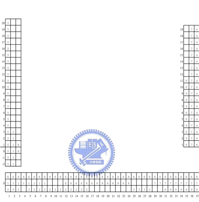
(26) ‧ ‧ 31 m ‧ ‧ ‧ ‧(37, 17) ‧ ‧ ‧ ‧ ‧ ‧ ‧ ‧ ‧ ‧ ‧ ‧ ‧ ‧(0, 10) ‧ ‧ ‧ 59 m ‧ ‧ ‧ ‧ ‧ ‧ ‧ ‧ ‧ ‧ ‧ ‧ ‧ ‧ ‧‧‧‧‧ ‧ ‧ ‧ ‧ ‧ ‧ ‧ ‧ ‧ ‧ ‧ ‧ ‧ ‧ ‧ ‧ ‧ ‧ ‧ ‧ ‧ ‧ ‧ ‧ ‧ ‧ ‧ ‧ ‧ ‧ ‧ ‧ ‧ ‧ ‧ ‧ (37, 0) (0, 0). Fig.4-2 Placement of BS on floor 8. Fig.4-3 Placement of BS on floor 9. To construct RADAR database, we choose these locations (x,y) in the middle of passages every 1.5 meter as in Fig. 4-2, roughly the distance per second one person can walk on a normal speed. At every location, we can detect from 1 to 3 base stations. In the area that has only one base station, handoff is unnecessary. Fig. 4-4 is the base stations at each location. We use different numbers 1, 2, …, 9 (ID of base stations) to identify different base stations.. 20.

(27) 20. 5. 19. 5. 19. 7. 4. 18. 5. 18. 7. 4. 17. 5. 17. 7. 4. 16. 5. 16. 7. 4. 15. 5. 15. 7. 4. 14. 5. 14. 7. 4. 13. 5. 13. 7. 4. 12. 5. 12. 7. 4. 11. 5. 11. 9. 7. 4. 10. 5. 10. 9. 7. 4. 9. 5. 9. 9. 7. 4. 8. 5. 8. 9. 7. 4. 7. 5. 7. 9. 7. 4. 6. 5. 6. 9. 7. 4. 5. 5. 5. 9. 7. 4. 4. 5. 4. 9. 7. 4. 3. 5. 1. 3. 9. 7. 4. 2. 5. 1. 2. 9. 7. 4. 1. 5. 1. 6. 1. 9. 7. 6. 0. 5. 1. 6. -1. 5. 1. -2. 5. 1. 6. 6. 6. 6. 6. 6. 6. 6. 1. 1. 1. 1. 1. 1. 1. 1. 5. 5. 5. 2. 2. 2. 2. 0. 1. 2. 3. 4. 5. 6. 7. 8. 6. 2. 6. 2. 6. 2. 6. 6. 6. 6. 6. 6. 6. 6. 6. 6. 6. 6. 6. 8. 8. 8. 8. 8. 8. 8. 8. 8. 8. 8. 8. 8. 2. 2. 2. 2. 2. 6. 3. 6. 3. 6. 3. 6. 3. 6. 6. 6. 6. 6. 6. 6. 6. 6. 7. 7. 7. 7. 7. 7. 7. 7. 7. 9. 9. 9. 9. 9. 9. 9. 9 10 11 12 13 14 15 16 17 18 19 20 21 22 23 24 25 26 27 28 29 30 31 32 33 34 35 36 37. Fig. 4-4 Number of base stations at chose locations. 4.2 Data Collection 4.2.1 RADAR’s Database To collect signal information, we use Wireless Valley’s LANFielder server and client as the measuring couple. LANFileder server is installed on a certain computer connected to TCP/IP network, and LANFielder client is installed on a laptop with Cisco350 WLAN card. After LANFielder server starts sending message packets through access points, LANFielder client starts to measure and record the RSS information of the associated AP. In all direction 21.

(28) (north, east, south, west) of every location, we recorded at least ten data and calculated the mean and variance of these data. Because the number of base stations are more than three, i.e. user will detect different base station in different locations, we have to record the ID of base station that we have measured. Thus we have a new form of the record tuple:. (x, y, n. BS. , BS1 , BS 2 , BS 3 , R 1 , V 1 , R 2 ,V 2 , R 3 ,V 3 , R 4 , V 4. ). where nBS is the number of base stations mobile user can detect, which maximum is 3, and BSi (i = 1, 2, 3) is the ID of base stations that can be detected, and. (R ,V ) = (rss , rss i. i. i. i. 1. 2. , rss i3 , var1i , var2i , var3i. ). where R and V are mean and variation of our calculated result and the superscript i denote the direction and the subscript discriminates different base stations.. 4.2.2 User Profile We select simplified tuple (x, y, x1 , y1 , x 2 , y 2 , x3 , y 3 , x 4 , y 4 ) to predicted next location. (x1, y1). (x4, y4). (x, y). (x2, y2). (x3, y3) We assume (x2, y2) = (x+1, y) (when the estimated direction is east). If (x+1, y) is not in our select locations, we assume(x2, y2) = (x, y). And then we assume (x1, y1) = (x, y+1), (x3, y3) = (x, y-1), and (x4, y4) = (x-1, y) in user profile as the same way.. 4.3 Simulation We can’t perform a real time experiment of location system like RADAR does because RADAR has to synchronize the beacons of all AP that that the mobile user can change channel periodically. Thus we perform only simulation of user’s walking through passageway.. 22.

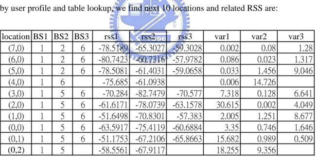
(29) To simulate the mobile user’s pace through passageway, first, we assign a path through passage. This path can be represented as locations from (0, 10) to (0, 0) to (37, 0) to (37, 17) to (37, 0) to (0, 0) to (0, 10), as shows in fig.4-2. Then we collect RSS data of these locations from the RADAR database that we constructed before. When we simulate the moving of mobile user, we give these RSS data plus a pseudo-noise (a normal distribution random number generated by computer multiplied by the standard deviation that we calculated before) to simulator and decide if handoff is made. At the end of every run, we record the numbers of handoffs and service failures. Every run under same experiment parameter repeated 100 times. Let’s take two examples to see how DP algorithm works. Example 1: no handoff is made. In location (0,3) with estimated direction of south, communicating base station ID = 5 by user profile and table lookup, we find next 10 locations and related RSS are: location BS1 BS2 BS3 (7,0) 1 2 6 (6,0) 1 2 6 (5,0) 1 2 6 (4,0) 1 6 (3,0) 1 5 6 (2,0) 1 5 6 (1,0) 1 5 6 (0,0) 1 5 6 (0,1) 1 5 6 (0,2) 1 5. rss1 -78.5189 -80.7423 -78.5081 -75.685 -70.284 -61.6171 -51.6498 -63.5917 -51.1753 -58.5561. rss2 -65.3027 -60.7316 -61.4031 -61.0938 -82.7479 -78.0739 -70.8301 -75.4119 -67.2106 -67.9117. rss3 -59.3028 -57.9782 -59.0658 -70.577 -63.1578 -57.383 -60.6884 -65.8663. var1 0.002 0.086 0.033 0.006 7.318 30.615 2.005 3.35 15.682 18.255. Table 4-1. Simulation result of DP process (1). 23. var2 0.08 0.023 1.456 14.726 0.128 0.002 1.251 0.746 0.989 9.356. var3 1.28 1.317 9.046 6.641 4.049 8.677 1.646 0.509.

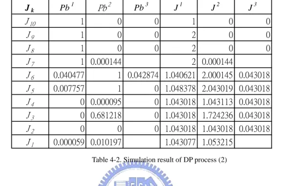
(30) Thus the probability of each rss below the threshold of service failure, and cost-to-go J at each stage are: (cost = 1). Pb 2. Pb 1. Jk. J 10 J9 J8 J7 J6 J5 J4 J3 J2 J1. Pb 3. J1. J2. J3. 1. 0. 0. 1. 0. 0. 1. 0. 0. 2. 0. 0. 1. 0. 0. 2. 0. 0. 1 0.000144. 2 0.000144. 0.040477. 1 0.042874 1.040621 2.000145 0.043018. 0.007757. 1. 0 1.048378 2.043019 0.043018. 0 0.000095. 0 1.043018 1.043113 0.043018. 0 0.681218. 0 1.043018 1.724236 0.043018. 0. 0 1.043018 1.043018 0.043018. 0. 0.000059 0.010197. 1.043077 1.053215. Table 4-2. Simulation result of DP process (2). Let’s define J i j as the element both on line J j and row J i and Pbi j is the element. (. ). both on the line Pb j and row J i . J i j is the expected value of J i j X i(1) , X i(2 ) , X i(3) , j . Thus at first we calculate J 10j , which are the probabilities Pb10j . Then to calculate J 91 ,. (. ). we must find min J 101 , J 102 + cost, J 103 + cost . These three elements of comparison have same. (. ). value, 1. Thus the expectation of J 91 X 9(1) , X 9(2 ) , X 9(3 ) ,1 is the sum of Pb91 and J 101 . J 92 and J 93 are calculated in the same way. Then, to calculate. (. J 81 we must find. ). min J 91 , J 92 + cost, J 93 + cost = (2,1,1) . Thus J 81 is calculated as sum of J 92 + cost and Pb81 . Other cost-to-go J i j could be computed as the same way. At last step, we compare J 12 and J 11 + cos t . Because J 12 = 1.053215 < 1.043077 + 1 = J 11 + cos t , no handoff is made.. 24.

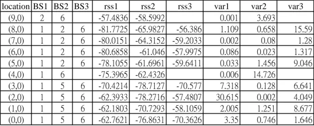
(31) Example 2: handoff is made: In location (0,1) with estimated direction of south, communicating base station ID = 5 by user profile and table lookup, we find next 10 locations and related RSS are:. location BS1 BS2 BS3 (9,0) 2 6 (8,0) 1 2 6 (7,0) 1 2 6 (6,0) 1 2 6 (5,0) 1 2 6 (4,0) 1 6 (3,0) 1 5 6 (2,0) 1 5 6 (1,0) 1 5 6 (0,0) 1 5 6. rss1 -57.4836 -81.7725 -80.0151 -80.6858 -78.1055 -75.3965 -70.4214 -62.3933 -62.1803 -62.7621. rss2 -58.5992 -65.9827 -64.3152 -61.046 -61.6961 -62.4326 -78.7127 -78.2716 -70.7293 -76.8631. rss3 -56.386 -59.2033 -57.9975 -59.6411 -70.577 -57.4807 -58.1059 -70.3626. var1 0.001 1.109 0.002 0.086 0.033 0.006 7.318 30.615 2.005 3.35. var2 3.693 0.658 0.08 0.023 1.456 14.726 0.128 0.002 1.251 0.746. var3 15.59 1.28 1.317 9.046 6.641 4.049 8.677 1.646. Table 4-3. Simulation result of DP process (3). Thus the probability of each rss below the threshold of service failure, and cost-to-go J at each stage are: Jk. J 10 J9 J8 J7 J6 J5 J4 J3 J2 J1. J1. Prob{rsss < Δ} 0 0.998929. 0. J2 0. J3 0. 0 0.000001 1.998929. 0 0.000001. 1. 0. 0. 2. 0 0.000001. 1. 0. 0. 2. 0 0.000001. 1. 0. 0. 2. 0 0.000001. 1 0.000526. 2 0.000527. 0.045096. 1 0.042874 1.045623 2.000527 0.043401. 0.011302. 1. 0 1.054703 2.043401 0.043401. 0 0.000066. 0 1.043401 1.043467 0.043401. 0 0.984272 0.000148 1.043401 2.027673 0.043549 Table 4-4. Simulation result of DP process (4). Because J 13 + cos t = 0.043549 + 1 < 2.027673 = J 12 , a handoff is made.. 25.

(32) 4.4 Numerical Result We compare our location-aware profile-based handoff algorithm with traditional (Hysteresis-Threshold) handoff algorithm. Some parameters in simulation are as follow: For Hysteresis-Threshold handoff algorithm: H = 3 (dB) (hysteresis), T = -72, -70 (dB) (threshold). For our algorithm: c = 0.5, 1, 1.5, …, 0.95, 1. n = 2, 3, 4, 10 (number of stages in DP algorithm) For both: Δ = -75 (dB) (threshold of service failure).. We performed simulation for each value of parameter over 100 times and compute their mean. The following graphs are the result of simulations.. 10 9 8 7. DP n=10. 6. DP n=4 DP n=3. 5. DP n=2. 4. T = -70 dB. 3. T = -72 dB. 2 1. 0.9 5. 0.8 5. 0.7 5. 0.6 5. 0.5 5. 0.4 5. 0.3 5. 0.2 5. 0.1 5. 0.0 5. 0. Fig.4-4 The number of handoff versus c (tradeoff parameter).. The number of handoffs in DP algorithm decreases when c increases from 0.05 to 1. This is because higher c means higher threshold of making handoff. Decrease of n from 10 to 2 does not change much of the number of handoffs. When T increases from –72 to –70(dB), the number of handoff of Hysteresis-Threshold algorithm increases almost two. 26.

(33) 4 3.5 3. DP n=10 DP n=4. 2.5. DP n=3. 2. DP n=2. 1.5. T = -70 dB T = -72 dB. 1 0.5. 0.9 5. 0.8 5. 0.7 5. 0.6 5. 0.5 5. 0.4 5. 0.3 5. 0.2 5. 0.1 5. 0.0 5. 0. Fig.4-5 The number of service failure versus c (tradeoff parameter). DP algorithm performs much better than Hyseresis-Threshold algorithm. This is because DP algorithm considers a number of future steps to compute best choice of handoff to avoid service failure. If we decrease n to 2, the number of service failure will increase when c is larger than 0.25 because the lack of future information.. 27.

(34) 14 12 10. DP n=10 DP n=4. 8. DP n=3 DP n=2. 6. T = -70 dB T = -72 dB. 4 2. 0.9 5. 0.8 5. 0.7 5. 0.6 5. 0.5 5. 0.4 5. 0.3 5. 0.2 5. 0.1 5. 0.0 5. 0. Fig.4-6 Bayes formula (c*handoff number + service failure number) versus c (tradeoff parameter).. DP algorithm is the best because of its best performance of service failure. Although n=2 in DP has almost the same performance as n=10, its higher service failure times suggests us to choose a higher n, say n=3, to keep lower number of service failure.. 28.

(35) Chapter 5 Conclusion. We introduced user profile and table lookup to overcome the problems of non-stationarity of user motion and signal strength history in predicting signal strength. Then we used these predicted signal information to perform DP algorithm. As the simulation result shows, DP solution outperforms over traditional method. To reduce computational load, we reduced n to 2. However, we must to make a tradeoff between the number of handoffs and service failure. Beside the tradeoff at small value of n, the DP algorithm with our method to predict signal information overwhelms the traditional algorithm in deciding handoff in WLAN.. 29.

(36) Reference [1] Paramvir Bahl and Venkata N. Padmanabhan, “RADAR: An In-Building RF-based User Location and Tracking System,” Proc. IEEE Infocom’00, March 2000. [2] Paramvir Bahl and Venkata N. Padmanabhan, “Enhancements to the RADAR User Location and Tracking System,” Microsoft Research Technical Report, February 2000 [3] Venugopal V.Veeravalli and Owen E. Kelly, “A Locally Optimal Handoff Algorithm for Cellular Communication,” Vehicular Technology, IEEE Transactions on, Vol. 46, No. 3, August 1997, p.p. 603 - 609 [4] W. Teerapabkajorndet and P. Krishnamurthy, “Throughput Consideration for Location-aware Handoff in Mobile Data Network,” Personal, Indoor and Mobile Radio Communications, 2002. The 13th IEEE International Symposium on , Volume: 5 , 15-18 Sept. 2002, Pages:2223 - 2227 vol.5 [5] W. Teerapabkajorndet and P. Krishnamurthy, “Comparison of Performance of Location-aware and Traditional Handoff-Decision algorithms in CDPD Networks,” Proc. IEEE VTC’01, Atlantic City, NJ, 2001 [6] Dimitri P. Bertsekas, “Dynamic programming and optimal control,” Athena Scientific, 2001, p.p. 1 - 30 [7] Kaveh Pahlavan, Prashant Krishnamurthy, and Jacques Beneat, “Wideband Radio Propagation Modeling for Indoor Geolocation Applications,” Communications Magazine, IEEE , Volume: 36 , Issue: 4 , April 1998, Pages:60 – 65 [8] T. S. Eugene Ng, Ion Stoica, and Hui Zhang, “Packet Fair Queueing Algorithms for Wireless Networks with Location-Dependent Errors,” INFOCOM (3), 1998, pages: 1103-1111 [9] Kaveh Pahlavan and Xinrong Li, “Indoor Geolocation Science and Technology,” IEEE Communication Magazine, February 2002, pages: 112-118 [10] Aysel Safak and Ramjee Prasad, “Effects of Correlated Shadowing Signals on Channel Reuse in Mobile Radio Systems,” Vehicular Technology, IEEE Transactions on , Volume: 40 , Issue: 4 , Nov. 1991, Pages:708 - 713 [11] K. S. Butterworth, K. W. Sowerby, and A. G. Williamson, “Correlated shadowing in an in-building propagation environment,” Electronics Letters , Volume: 33 , Issue: 5 , 27 Feb. 1997, Pages:420 - 422 [12] Nissanka B. Priyantha, Anit Chakraborty, and Hari Balakrishnan, “The Cricket Location- Support System,” 6th ACM/IEEE International Conference on Mobile computing and Networking (ACM MOBICOM ’00) [13] Jeffrey Hightower and Gaetano Borriello, “A Survey and Taxonomy of Location Systems for Ubiquitous Computing,” Technical Report UW-CSE 01-08-03, August 24, 30.

(37) 2001 [14] Theodore S. Rappaport, “Wireless Communications,” 2nd edition, Prentice Hall [15] Brian P. Crow, Indra Widjaja, Jeong Geun Kim, and Prescott T. Sakai, “IEEE 802.11 Wireless Local Area Networks,” IEEE Communications Magazine, September 1997. 31.

(38)