Generalized hold function design for periodically time-varying systems

Proceedings of the American Controi Conference Philadelphia, Pennsylvania June 1998

Generalized Hold Funtion Design

For Periodically Time-Varying Systems

Min-Shin Chin

Department

of

Mechanical Engineering

National Taiwan University

Taipei, Taiwan, Republic

of

China

TEL:02-3630231 ext. 2414

EMAIL:[email protected]

FAXrO2-3631755

Abstract- Most control designs for periodically time-varying systems use either full state feedback or observer-based state feedback. In this paper, it is shown that statzc output feedback is sufficient for the exponen- tial stabilization of a periodical system under both the controllability and observability assumptions. In fact, by incorporating a new generalized hold function in the control design, one is able to arbitrarily shift all the Poincare' exponents of the periodical system. Most im- portantly, the control singal is guaranteed t o be con- tznuous in time while the control signal from previous designs may be discontinuous.

1

Introduction

An important class of linear time-varying systems in the physical world is the class of periodical systems, in which the system parameters vary periodically. Anal- ysis for such systems has been done thoroughly in the past [1,2]. One of the most important results is sum- marized in the Floquet theory, which states that the stability property of a linear periodical system can be determined by n constant numbers called the Poincare' exponents, where n is the dimension of the system. If all the Poincare' exponents are in the open left-half plane, t,he periodical system is exponentially stable. If a t least one of the Poincare' exponents is in the open right-half plane, the system is unstable.

control designs are based on the assumption that all the state variables are accessible for measurement. Among t~hese, the earliest approach is the LQ optimal control, in which one solves a periodical Riccati equation to ob- tain a stabilizing state feedback control [3,4]. Another approach is t h e modal control proposed in [ 5 ] , which can

arbitrarily shift only one of the Poincare' exponents of

For the stability synthesis of periodical systems, most

the system. Later, a layer of modal controllers are sug- gested t o shift all the Poincare' exponents [6]. Recently, the generalized hold function design, originally devel- oped in [7], is applied to the state feedback control of a

periodical system [ 8 ] . However, the resultant control sig- nal may have large discontinuities in time. In practice, such large discontinuities are either unacceptable under the actuator constraint or undesirable due to the possi- ble excitation of high frequency unmodelled dynamics. Even though an attempt has been made to make the control signal continuous, its success is obstructed by a

singularity problem [8].

In this paper, a new design is proposed to avoid dis- continuities in the control signal. Furthermore, it is shown that when the periodical system is both con- t,rollable and observable, simple static output feedback control is sufficient for the arbitrary assignment of all the Poincare' exponents (note that full state feedback is required in [8]). The key elements in the new con- trol design are the well-known Floquet transformation [5] and a new generalized hold function design [7]. This paper is arranged as follows. In Section 2, the definition

of Poincare' exponents for a periodical system is pre- sented. In Section 3 , a discontinuous output feedback control is developed to assign the Poincare' exponents of the closed-loop system, and the control design is further modified in Section 4 in order to remove discontinuities in the control signals.

2

Stability Analysis

for

Periodical Systems

Consider the stability analysis of the following system k ( t ) = i l ( t ) z ( t ) , (1) where z ( t ) E

R"

is the state vector, the system matrix

A ( t ) E

R T L X X "

is T-periodic in the sense that A ( t

+

T) =

A ( t ) ,

V

t

>

0.

In the famous Floquet theory [l], the stability prop- erty of (1) is studied through a state transformation into

a new coordinate, on which the system matrix becomes time invariant. Such a transformation, called the Flo- quet transformatzon, is given by

~ ( t ) = ~ ( t ) x ( t ) , ~ ( t )

=

eJt@-' (tl O ) , (2) where @(t,O) is the state transition matrix [2] of (l), and J is a constant matrix given by

(3)

1 T

J =

-

In@(T,O).

From ( l ) , (2) and (3), the periodical system (1) has a constant representation in the new coordinate:

i ( t ) = J z ( t ) . (4)

One can verify (see

[a])

that the state transformation matrix P ( t ) in (2) is also T-periodic, and remains uni- formly bounded and nonsingular. The stability property of the periodical system (1) can then be inferred from that of the constant system (5). In the literature, the eigenvalues of the constant matrix J in (5) are referred as the Potncari (or characterastac) exponents

(5)

A 1

T

P.E. = X,(J) =

-

InA,[@(T,O)],

where the second equality results from

(3).

The condi- tion for exponential stability of (1) is thus

Re[A,(J)]

<

0, (6)

or equivalently.

I & [ W , O ) I l

<

1,

due to (5), where @(T,O) is called the monodromy ma- trzx 181. To end this Section, note that from (2) and (3)

one can derive the identity

@(T,

t ) =

e J ( T - t ) P ( t ) , which will be used in subsequent Sections.

3

Stability Synthesis

by

Discontinuous Control

Consider now a periodical system with control

i ( t )

= .4(i)z(t) t B ( t ) u ( t ) ,

x ( 0 )

=

2 0 , Y ( t ) = C ( t ) Z ( t ) ,

where

~ ( t )

E

R"

is the state vector, u ( t )

E

RP the con- trol input, and y(t) € Rq the system output. It is as- sumed that the only accessible signal is the systern out- put y ( t ) , and that A ( t ) E

R n X " , B ( t )

€

RnXP,C(t)

E

Rqxn are all T-periodic; i.e.,

( A ( t + T ) , B(t+T), C(t-tT)) ( A ( t ) , B ( t ) ,

C ( t ) )

'dt > 0

The objective in this Section is to find a stabilizing static output feedback control u ( t ) that can arbitrarily assign the locations of the Poincare' exponents of the closed- loop system. For this purpose, the following assump- tions are required:

( A l ) The pair ( A ( t ) , B ( t ) ) is controllable in the sense that its controllability grammian [l] W defined on the time interval [0, T ] is positive definite, where

and @ ( 1 , T ) is the open-loop state transition matrix of

(A2) The constant pair (@(T, 0),

CO)

is observable [9],

where @(T, 0) is the open-loop monodromy matrix, and

(1).

CO

=

A C ( 0 )

=

C(kT).

The proposed control design proceeds as follows.

Step I. Choose n Poincare' exponents w, (real or in complex conjugate pairs) with Re(w,)

<

0. Calculate the eigenvalues for the closed-loop monodromy matrix based on

(5):

A;

=

P I , (10)

and then use the pole placement algorithm [9] to find a constant matrix L E R"'Q so that

& ( @ ( T , 0 )

+

LCo) = A;, (11) where @(T, 0) and CO are as in Assumption (A2). Note that Assumption (A2) guarantees the existence of L in

(12) for any choice of the value

At.

Step 11. Construct a 7'-periodic generalized hold func- tion

G ( t )

E

RPxQ

with

G(t

+

T )

=

G ( t ) ,

and

G ( t )

=

B T ( t )

QT(?',t)

W-I L ,

t

E

[O,T),

(12)

where (P(T,t) and W are as in (9). Note that Assump- tion (AI) guarantees the invertibility of W .

Step 111. Set the control input to be

u ( t )

=

G ( t ) y ( k T ) ,

t

E [kT, kT

+

T ) , (13)

where y ( k T ) is the sampled system output with a sam-

Notice that in the above control design, one needs t o calcula.te the open-loop state transition matrix

@(T,

7 )

over the entire period r

E

[O,T]. Such computation becomes difficult when the period is long or when the system dimension is large. For an efficient and accurate numerical algorithm in calculating the state transition matrix, one may refer t o [1O,11].

Theorem 1 : Under the Assumptions ( A l ) and (A2),

the static output feedback control (13) stabilizes the system (8) exponentially. Furthermore, the closed-loop Poincare' exponents are located as specified in Step I in the design procedure.

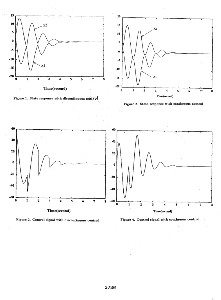
A simple simulation example is provided below t o ver- ify the proposed control design.

Example 1 : Consider a periodic system, which is open-loop unstable,

y ( t ) =

[

2

+

sin4xt -9

+

sin4xt

]

~ ( t ) .

The period of the system is one second. T h e proposed control ( 1 3 ) is applied t o the system with the initial condition xT(0)=[2,

21.

T h e design parameters in Step

I are w1 = lnO.l and w2 = ln0.3. Figure 1 shows the

time history of the system state, which converges expo- nentially as predicted by Theorem 1, and Figure 2 shows the control input.

4

Stability Synthesis by

Continuous Control

Figure 2 in Example 1 reveals a problem with the control design based on the generalized hold function: the control signal u ( t ) in (13) has large discontinuities at

the sampling instants t = k T . Since control with large discontinuities is either not implementable in practice

or unacceptable from the robustness consideration, the objective of this Section is t o modify the previous control design so that assignment of the Poincare' exponents can be achieved by a continuous control input.

T h e approach adopted here is t o find a new general- ized hold function

G ( t )

t o replace

G ( t )

in the discontin-

uous control

(13), with

G ( t )

now satisfying

G ( t T )

=

0,

v k =

0 , 1 , 2 , .

. .

(14)

This will force the control input u ( t ) t o be continuous at any time instant

t

= k T ; in fact, according t o ( 1 3 ) and (14) ~ one has

u ( t - ) = U @ + ) = 0 , at t = k T . (15)

T h e modified design procedure is as follows.

Step I and Step I1 are the same as in the previous

Section.

Step 111. Choose any two T-periodic matrix functions G l ( t ) E RPxq and G z ( t ) E

RPxq

t h a t are continuous on ( 0 , T ) . Calculate R[Gl(r)] and R[G2(r)], where R[.] is the controllability map

T

R [ G i ( r ) ] =

1

@(T

T ) B ( T ) G $ ( ~ ) ~ T . Denote the two resultant constant matrices by

L1 R [ G l ( r ) ] E

Rnxq,

L2

e

R[G2(r)] E

Rnxq.

(16)

Step IV. Construct the following two T-periodic matrix functions from G l ( t ) and G2(t),

t

E [O,T),

Gol(t) = G l ( t ) - BT(t)@'(T,t)W-' L1, (17) Goz(t) = G2(t) -

B T ( t ) a T ( T , t ) W - '

La, (18) where B ( t ) ,

@ ( T , t ) ,

and W are as in (12), and L1 and L2 in (16).

Step V. Case (a). When the number of inputs are no less than t h a t of outputs ( p

2

q ) , determine two constant matrices a1 and a2 E

RPxp

from the equations

G(O+)

+

aiGoi(0')

+

a2G02(Ot)

= 0,

(19)

G(T-)

+

aiGoi(T-)

+

~ 2 G o 2 ( T - ) =

0,

(20)

where G ( t ) is given by (12), and Gol(t) and Go2(t) by (17) and (18). Solutions a1 and a2 in (19) and (20) exist

if the following matrix is full rank

If this condition is not satisfied for the G l ( t ) and G2(t) chosen in Step 111, one can simply choose a different pair of G l ( t ) and Gz(t) until the required rank condi- tion is satisfied. Notice t h a t there are znfinzte degrees of freedom in choosing G l ( t ) and G2(t) for no constraint is imposed on them except continuity on the interval ( 0 , T ) . Hence, choosing G l ( t ) and Gz(t) t o meet the above rank condition is in general quite easy.

Case (b). When the number of inputs are no more than t h a t of outputs ( p

5

4 ) , determine two constant matrices ,D1 and p2 E Rqxq from the equations

G ( T - )

+

Goi(T-)Pi

+

G o z ( T - ) P 2 = 0 , where G ( t ) , Gol(t) and G02(t) are as in (19). Similarly, it will be assumed t h a t in solving the a.bove equations for

/31 and

,&,

the following matrix (note that it is different from the previous one) is full rank

S t e p VI. Set the control input to be

u ( t ) = G ( t ) y ( k T ) , t E

[kT,

kT+

T ) , (21) where y ( k T ) is the sampled system output, and G ( t ) = G‘(t

+

T ) is the new generalized hold function

G ( t )

G ( t )

+

aiGoi(t)

+

azGoz(t), if P

L

q

G ( t ) = G ( t )

+

Goi(t)Pi

+

G02(t)Pz, if P

I

q ,

in which

G ( t ) ,

Gol(t),

Goz(t)

are as in (19), and ai and

Pt

from Step V.

The following theorem shows that the new control (21) will shift the Poincari exponents to the same de- sired locations as the discontinuous control (13) in the previous Section; furthermore, the new control input (21) is now continuous for all

t

>

0.

Theorem 2 : The closed-loop system (8) with the con- tinuous control (21) is exponentially stable. Further- more, the closed-loop Poincare‘ exponents are located as specified in Theorem 1.

Example 2 : In this Example, the contznuous control

(21) is simulated for the same system as in Example 1. The control design parameters in Step I are as before, and the T-periodic functions ( T = l second) in Step I11 are chosen to be G l ( t )

= t , Gz(t) =

1

-

t ,

where

t

E

[O, T ) . Figure 3 shows the time history of the controlled system state, and Figure 4 the control input. Observe that the control input now becomes continuous in time while the state convergence rate remains the same as in Example 1.

References

111

E.

A. Coddington and N. Levinson, Theory of

Or-

dinary Dzfferential Equations, McGraw

Hill,

New York, 1955.

[a]

F.

Callier and

C.

A. Desoer, Lznear System Theory, Springer-Verlag, Hong Kong, 1992.

[3]

S.

Bittanti, P. Colaneri, and

G.

Guardabassi, ”Anal- ysis of the periodic Liapunov and Riccati equations via canonical decomposition,” SIAM. J . Control and Opti- mization, vol. 24, pp.1138-1149, 1986.

[4] H. Kano, and

T.

Nishimura, ”Periodic solutions of matrix Riccati

equations

with

dectectability and stabilz-

ability,” Int. J. Control, vol. 29, pp.471-487, 1979.

[5]

R.

A . Calico, and W. E. Wiesel, ”Control of time- periodic systems,” J . Guidance, vol. 7, pp.671-676, 1984.

[6] S. G. Webb,

R.

A. (Calico, and W. E. Wiesel, ”Time- periodic control of a multiblade helicopter,” J . Guid- ance, vol. 14, pp.1301-1308, 1991.

[7] A. B. Chammas, and

C.

T . Leondes, ”On the design of linear time invariant systems by periodic output feed- back, Part I and 11,” Int. J . Control, vol. 27, pp.885-903, 1978.

[8] P. T. Kabamba, ”Monodromy eigenvalue assignment in linear periodic systems,” IEEE Trans. on Automatic Control, AC-31, pp.950-952, 1986.

[9] T. Kailath, Lznear Systems, Prentice-Hall, Engle- wood Cliffs, New Jersey, 1980.

[lo] S. C. Sinha, and 13-H, Wu, ”An efficient computa-

tional scheme for the analysis of periodic systems,” J . Sound and Vibration, vol. 151, pp.91-117, 1991.

[11] S. C. Sinha, D-H. Wu, V, Juneja, and P. Joseph, ”Analysis of dynamic systems with periodically varying parameters via Chebyshev polynomials,” J . Vibration and Acoustics, vol. 115, pp.96-102, 1993.

15 LO 5 0 -5 -10 -15 -Xl

1

-20 0 1 2 3 4 5 6 7 8 Time(second)

Figure 1. State response with discontinuous cohtro/

60 40 20 0 -20 a0 -60 0 1 2 3 4 5 6 7 8 Time(second)

Figure 2. Control signal with discontinuous control

20 15 LO 5 0 -5 -10 -15 -20 0 1 2 3 4 5 6 7- 8 Time(seeond)

Figure 3. State response with continuous control

60

0 I 2 3 4 5 6 7 8

Time(second)