國
立
交
通
大
學
資訊科學與工程研究所
碩
士
論
文
於 資 料 串 流 上 基 於 動 態 網 格 的 分 群 演 算 法
Clustering Evolving Data Stream Based on Dynamic Grids
研 究 生:王偉任
指導教授:李素瑛 教授
二
於資料串流上基於動態網格的分群演算法
Clustering Evolving Data Stream Based on Dynamic Grids
研 究 生:王偉任 Student:Wei-Jeng Wang
指導教授:李素瑛 Advisor:Suh-Yin Lee
國 立 交 通 大 學
資 訊 科 學 與 工 程 研 究 所
碩 士 論 文
A ThesisSubmitted to Institute of Computer Science and Engineering College of Computer Science
National Chiao Tung University in partial Fulfillment of the Requirements
for the Degree of Master
in
Computer Science
June 2012
Hsinchu, Taiwan, Republic of China
i
於資料串流上基於動態網格的分群演算法
研究生:王偉任
指導教授:李素瑛
國立交通大學資訊科學與工程研究所摘要
近年來,由於資訊科學的發展和相關設備的進步,資料串流已成為普遍的 資料型態。如何在無限且動態的資料串流上進行分群,並擷取出有意義的資料特 徵,此問題已經引起重大的關注。雖然在此議題上已有相當的研究發表,多數的 方法都需要在起始時給予適當的參數設定。然而在資料串流上,與一般靜態的資 料不同,其資料特徵與分群資訊是動態而不穩定的,因此在起始的參數設定相當 困難。處理資料串流是一個連續的程序,在不同時刻也可能需要不同的參數設定, 固定參數的方法往往在其資料特徵改變時無法正確的反映與處理。本篇提出一個 新穎的演算法,DGBC (動態網格分群法),用來對資料流進行分群。在過程中,該 方法可以自動的調整所需要的參數,用以對應最新的資料與分群特徵。在合成資 料和真實資料兩者上所進行的實驗結果均顯示 DGBC 不僅擁有較快的執行速度, 所產生的分群結果也有較高的品質,同時對於起始參數的敏感度也較低。ii
Clustering Evolving Data Stream Based on Dynamic Grids
Wei-Jeng Wang
Suh-Yin Lee
Institute od Computer Science and information Engineering
National Chiao-Tung University
Abstract
Clustering multi-dimensional data stream is a difficult and important problem. The goal is to cluster the objects within the stream continuously, to discover and monitor the evolving up-to-dated events. Density grid based clustering algorithms are fast, and can discover arbitrarily shaped clusters and deal with noise. However, the sizes and borders of the grids easily influence Grid-based algorithms. We propose a Dynamic Grid-Based Clustering algorithm for high-dimensional data streams. When new data arrives, the grid structure is dynamically updated. Dynamic grid structures adjust its range and boundary on each dimension over time to produce effective clustering results with low memory usage. We used both synthetic and real data set for experiments, and the experimental results show that our proposed algorithm has superior quality and efficiency, can find clusters of arbitrary shapes, and can accurately recognize the evolving behaviors of real-time data stream
iii
ACKNOWLEDGEMENT
I greatly appreciate the kind guidance of my advisor, Prof. Suh-Yin Lee. She not only helps with my research but also takes care of me. Her graceful suggestion and encouragement help me forward to complete this thesis.
Besides, I want to give my thanks to all members in the Information System Laboratory for their suggestion and instruction. Especially Mr. Yi-Cheng Chen, Mr. Fan-Chung Lin, and Mr. Li-Yen Qua.
Last but not least, I appreciate my parents. Without their support and encouragement, I am not able to complete achievement. I devoutly dedicate this thesis to them.
iv
Table of Contents
Abstract (Chinese)……..…………...……….………..i Abstract (English)..……..…….……….….ii ACKNOWLEDGEMENT….………...……….iii Table of Contents……..…….………..……….ivList of Figures ……….…..……….….……….……...………vi
List of Tables …………..…..………..……….……..……viii
Chapter 1 Introduction ……...….………..1
Chapter 2 Related Works ……….………..3
2.1 Clustering Algorithm on Data Stream ….………...……….……….……..3
2.2. Evolving Approach ………..……….…….…...……… 4
2.2.1 Micro-Cluster Distance Factor …………..…...……… 4
2.2.2 Micro-Cluster Density Factor ………..………. 7
2.2.3 Density Grid Density Factor…… ……….………..…….…. 8
2.3 Indexing Structure...……….……….………. 12
2.3.1 R-tree ………...………. 12
2.3.2 R+ tree ……….…. 12
Chapter 3 Notation and Problem Definition ………. 14
3.1 Notation and Symbol Definition ………...…………. 14
3.2 Problem Statement ………. 18
Chapter 4 Dynamic Grid-Based Clustering ……….…. 19
4.1 Overview of DGBC ………..…. 19
4.2 Indexing ………....………..………... 20
v
4.2.2 Dimensional Interval Based-Indexing ……….……. 22
4.3 Maintenance Step and Grid Resizing ……….………...……….24
4.4 Cluster Generation……….………..….……. 26
4.5 Decay Factor, Threshold, and Time gap ………….………..………. 27
4.6 DGBC algorithm ………...…………. 33
Chapter 5 Experimental Results ……….…………...………. 35
5.1 Cluster Quality ………..……. 35
5.2 Data Generator ……….……. 36
5.2.1 Performance on Synthetic Datasets …….………….……… 37
5.2.2 Scalability Studies ……….………..…. 39
5.3 Network Intrusion Detection dataset ……….……….…….……. 41
5.3.1 Performance on Network Intrusion Detection dataset ……….…….…… 42
5.4 Charitable Donation data set ………..………… 43
5.4.1 Performance on Charitable Donation dataset ………...……...…. 44
5.5 Parameter Analyze ……….…………..…... 45
Chapter 6 Conclusion ……….……… 49
vi
List of Figures
Figure 2.1 Process of distance-based micro-clusters method……...…….………..5
Figure 2.2 Process of density-based micro-clusters methods……...………...7
Figure 2.3 Process of grid based method with density factor………..9
Figure 4.1 Illustration of DGBC………19
Figure 4.2 An example for R+ tree-based index………21
Figure 4.3 An example for dimensional interval-based index………...23
Figure 4.4 The pseudo code of DGBC………...34
Figure 5.1 Example for compute purity……….36
Figure 5.2 Quality comparison (Synthetic dataset)………38
Figure 5.3 Execution time comparison (Synthetic dataset)………...39
Figure 5.4 Scalability test with different number of dimensions (Synthetic dataset)40 Figure 5.5 Scalability test with different number of clusters (Synthetic dataset)…..41
Figure 5.6 Quality comparison (Network Intrusion dataset)……….42
Figure 5.7 Execution time comparisons (Network Intrusion dataset)…………..….43
Figure 5.8 Quality comparison (Charitable Donation dataset)………..…44
Figure 5.9 Execution time comparisons (Charitable Donation dataset)………45
Figure 5.10 Cluster Quality with different initialization (Network Intrusion dataset)………..46
Figure 5.11 Cluster Quality with different initialization (Charitable Donation dataset)….……….47
Figure 5.12 Execution time with different initialization (Network Intrusion dataset)….……….47
vii
Figure 5.13 Execution time with different initialization (Charitable Donation
viii
List of Table
1
Chapter 1
Introduction
In recent years, advances in hardware technology have allowed us to automatically record transactions at a rapid rate. They are massive, fast changing, and infinite. These data processes are referred to as data stream, data that is coming in a continuous flow, is generated nonstop at a rapid rate from sensors and mobile applications, log records, click-stream in web exploring, etc.
Clustering data streams posed additional challenges such as: single pass, limited time and memory, and evolving clusters. The clustering result can be used to gain insight into the distribution of data, to observe the characteristic of each cluster, or a particular set for further analysis. The goal is to cluster the objects within a stream continuously, and to discover and monitor the evolving up-to-dated result.
Many steam clustering algorithms have been proposed. Some of the methods that developed are distance-based. They are suitable to find well convex clusters with flexible memory requirement. However, for non-convex clusters, these methods have trouble finding the true clusters, since two points from different clusters may be closer than two points in the same cluster.
Another type of streaming clustering is the hybrid of density-based and grid-based method [6] [9] [10] [20]. A Grid-based method maps data into corresponding discretized density grid and the density factor connects the high density objects to generate the clusters. It is a fast approach due to the low mapping cost. Nevertheless, since the characteristics of data stream may change over time, a static grid boundary may not be suitable for all the time points. When the data property is changed, different
2
setting is needed to produce effective and meaningful result.
We propose a Dynamic Grid-Based Clustering (DGBC), an algorithm for clustering high-dimensional data streams. It is a density based algorithm for clustering streaming data with the grid structure. It benefited by the density factor that can find clusters with arbitrary shape, and can deal with outliners and is less sensitive to the ordering by the density grid structure. Since data stream can change its property over time, we may need different parameters at different time point to generate effective and meaningful result. The grids are not partitioned at the start of process, but are adjusted over time depending on the characteristic of data. At different time stamp, a different grid size is computed and assigned to produce high quality result.
As the grids now are created and deleted over time, it cannot be directly access. We use an indexing to keep and search the grid list efficiency. The index can help us not only speed up the searching operation, but also reduce time when merging the grids at the clustering stage.
We also use decay factor to address the evolving concept in stream data. We put more weight on the current data without discarding the historical information. As a fading window model, it is a popular method to deal with stream data.
The rest of this thesis is organized as follows. Chapter 2 provides the related works. Chapter 3 presents the notation and problem definitions. Chapter 4 describes the details of our proposed algorithm. Chapter 5 presents the experimental result and performance study. The conclusion and the future work are in Chapter 6.
3
Chapter 2
Related Work
In this chapter, we introduced the related works of this thesis. In Section 2.1, we classified the existing work on streaming clustering into several types by the summary structure they use and the factor they choose to produce clustering result. Section 2.2 describes the index structure we use in this thesis.
2.1 Clustering Algorithm on Data Streams
Based on the concept of processing data stream, previous algorithms on clustering data streams can be classified into two categories: one-pass approach and evolving approach. Here we will introduce the one-pass approach and focus on the evolving approach in the following section.
The one-pass approach extends traditional clustering methods [5] [15] by scanning data once only. These methods extended the k-means or k-median, and maintained the intermediate results of clustering algorithms over all time points. Such an approach is highly sensitive to the order of arrival of the data points, especially when the characteristics of a stream evolve over time. BIRCH [25] uses a cluster feature summarization methodology, STREAMLS [17] uses a modified LSEARCH to find the center candidates for the clusters, and STREAM collects the result of k-median on every time point.
DUC-Stream [10] is a single pass clustering algorithm for data streams. It is a density grid based method. The data stream is read in chunks. Each chunk fits in the memory and contains a number of data points. It partitions the data domain into units
4
and keeps only the units that have a large number of data. If a unit has more data points than the threshold, the unit will be considered as a dense unit. A local dense unit is a candidate for dense unit which may become a dense unit.
DUC-stream keeps the dense units and the current local dense units. In the process, it takes a chunk of data points, map them into corresponding units, and then find the local dense units at the current time point. It generates the clustering result in an incremental manner. DUC-stream identifies the clusters as a connected component of a graph in which vertices represent the local dense units and the edges are related to common attributes between two vertices. After the current clusters are created, they are merged with the result created before. For each added dense unit, if it has no common dimension boundary with any existed clusters, a new cluster is generated and merges the dense unit into it. Or if there are any clusters that have common dimension boundary with the new dense unit, then merge the dense unit into the cluster. A cluster will be deleted if it contains no dense unit.
2.2 Evolving Approach
The evolving approach takes the streams as an evolving process over time. They try to discover not only the cluster result at the last time point but also the data evolving during the process. There are three types of algorithms according to the similarity measurement and the summary structure they use: distance-based with micro-clusters, density-based with micro-clusters, and density-based with density grids.
2.2.1 Distance-Based Micro-Clusters Methods
This type of method uses micro-cluster as the summary structure to store the data information. A distance based algorithm like K-means can be used to generate the
5
final clustering result. A micro-cluster contains the cluster feature vector as MC = {N, LS, SS}, where N is the number of data in the micro-cluster, LS is the linear sum on each dimension and SS is the square sum on each dimension.
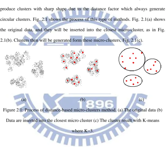
Micro-cluster can provide a flexible memory usage by controlling the maximum number of micro-clusters and can find well convex clusters, but can not produce clusters with sharp shape due to the distance factor which always generate circular clusters. Fig. 2.1 shows the process of this type of methods. Fig. 2.1(a) shows the original data, and they will be inserted into the closest micro-cluster, as in Fig. 2.1(b). Clusters then will be generated form these micro-clusters, Fig. 2.1(c).
(a) (b) (c)
Figure 2.1: Process of distance-based micro-clusters method. (a) The original data (b) Data are inserted into the closest micro cluster (c) The cluster result with K-means
where K=3.
CLUStream [3] is a clustering algorithm for streaming data. The clustering process is divided into online component and offline component. The online component stores summary information by micro-clusters and the offline component analyzes the data streams over different horizons by using summary information which is stored in online component. When a new data arrives, the algorithm will find the closest
6
micro-cluster, and insert the data if the distance between the data and the center of micro-cluster is under the threshold. A new micro-cluster is created if the new data dose not lie within the maximum boundary of the nearest micro-cluster. An old micro-cluster will be deleted or the closest two micro-clusters will be merged to control the number of micro-clusters. At the clustering step, micro-clusters are treated as pseudo-points, and a modified k-means is used to generate the clustering result.
The micro-clusters are stored at snapshots in time which follow a pyramidal pattern, to keep the cluster information at different points. The summary information is used by offline component when a user required the clustering result in a time horizon or granularity. CLUStream can find well convex clusters with flexible memory requirement, and provides a wide variety of functionality in characterizing data stream clusters over different time horizons in an evolving environment.
SWClustering [26] algorithm uses Exponential Histogram of Cluster Feature (EHCF) to maintain the cluster features over a sliding window. Temporal Cluster Feature (TCP) is used to keep the cluster feature vector at each time stamp, and a micro-cluster here is a set of TCP that are close to each other. When more data come, old TCPs are merged to generate TCP that keeps larger time interval data. The TCP structures record the evolution of each cluster and capture the distribution of recent records. TCP structure supports record-level clustering analysis since it creates a TCP for every newly arrived record. As each EHCF has its own temporal feature, two EHCFs can not be merged directly if two EHCFs are overlapping, i.e., the arrival time of the record in two EHCFs are interleaved. It uses late merging to deal with the case. A new EHCF is created conceptually to merge the interleaved EHCFs to keep all the information. It has a better quality and higher time complexity since it has to process the
7
historical buffer.
2.2.2 Density-Based Micro-Clusters Methods
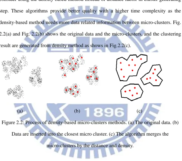
As the density measurement can not find sharp clusters, some algorithms consider using the density based method instead of distance factor in cluster generating step. These algorithms provide better quality with a higher time complexity as the density-based method needs more data related information between micro-clusters. Fig. 2.2(a) and Fig. 2.2(b) shows the original data and the micro-clusters, and the clustering result are generated from density method as shows in Fig.2.2(c).
(a) (b) (c)
Figure 2.2: Process of density-based micro-clusters methods. (a) The original data. (b) Data are inserted into the closest micro cluster. (c) The algorithm merges the
micro-clusters by the distance and density.
In DenStream [6], instead of using the number of neighboring data points stored in the micro-clusters, micro-cluster density is based on weighting areas of points in the neighborhood. It has online-offline components. In evolving data streams, the role of clusters and outliers may change over time. There are three types of micro-cluster: p-micro-cluster, o-micro-cluster and c-micro-cluster. c-micro-cluster means
8
core-micro-cluster, a type of micro-cluster that their density weight is higher than the threshold. o-micro-cluster means outlier-micro-clusters, their density weight is lower than the threshold. p-micro-cluster means potential-c-micro-cluster, they are not core micro-cluster now, but their density weights is higher than the low threshold and may become a c-micro-cluster some time later.
When a new data comes, first the algorithm tries to merge with the closest p-micro-cluster. Otherwise, the data will be merged with the closest o-micro-cluster or new an o-micro-cluster for it. If the density weight of a p-micro-cluster is higher than the threshold after the insertion, that p-micro-cluster becomes a c-micro-cluster. On the clustering stage, a variant of DBSCAN algorithm is applied to the p-micro-clusters to get the final result.
SDStream [14] algorithm is based on SWClustering algorithm and DenStream. SDStream assigns a weight based on the number of data points in the c-micro-cluster, p-micro-cluster, and o-micro-cluster. The micro-clusters are stored in the form of EHCFs, like in SWClustering, recording the evolution of each cluster and capture the distribution of recent records. The final clusters are generated based on these virtual points using modified DBSCAN.
2.2.3 Density-Based Density Grids Methods
Density grid is a fast approach for recording the drift information. This type of methods divides the data domain into grids and records the data that fit in each grid boundary. These methods are insensitive to the outlines and noises, since the new data would not change the grid structure and neither cause old structure deleted as we need to control the maximum number of structure. This is also less sensitive to the incoming data order
9
since we do not update the grid center for every incoming data. By merging the grids, these methods can find arbitrary shape clusters, and find boundary or outliner data fast. Fig. 2.3(a) and Fig. 2.3(b) show the original data and the density grids. The method then find high dense grid and generates clusters as shown in Fig. 2.3(c) and Fig. 2.3(d).
(a) (b) (c) (d)
Figure 2.3: Process of grid based method density factor. (a) The original data. (b) Data are mapped into the density grid unit. (c) Find out and store the high density units. (d)
The neighboring high density grids are merged and three clusters are generated.
However, the number of grids easily increases especially when dealing with high dimensional data. These methods partition the data domain in the initialization step, a good result depends on a good partition setting, and in most of cases it is hard to decide as there is no information about the data distribution and cluster features. Even if we can get a good setting at the start stage, the data property may change over time during the streaming process, and we may not always have a good parameter for every time point.
Chen et al. proposed a framework called D-Stream [7] for clustering data streams based on density. Density is defined as the number of data fall in a specific area.
10
D-Stream also has online-offline components. The online component reads new data records and maps them into density grids and updates summary information about the grids. Based on grid density, dense and sparse grids are introduced. Their difference is referred to their density. A dense grid is that its density is higher than threshold, and a sparse grid is a grid that its density lowers than the low threshold. It also uses a decay function to express the concept of stream evolving, as we consider that the new data are more important than the old ones. A grid that dose not receive data for a time period will become sparse, and its density should be low even if it was a high dense grid before. The offline component clusters the density grids by connecting each high-dense neighboring grids. A grid cluster is a connected grid group, which has higher density than the threshold. It is a fast approach due to the low mapping cost, and can find arbitrary shape clusters.
In [24], Tu et al. improved the D-Stream by considering the positional information about the data. When mapping data into grids, the gird structure keeps the attraction information which shows how close a data to its neighbors. The clustering procedure is the same as before. The difference is at the merging step. Two grids will be connected only if they are both high-density grids and their attraction is higher than the threshold. By considering the density and attraction, this algorithm has a better cluster quality.
AGD-Stream [8] is a density grid based method which considers the idea of activity and boundary data. A grid is active if it has received new data at some time points, and the active grids should be kept. We need only check a grid if it is active when it receives a new data, or when a user sends a query. Another idea is the boundary grids. A data is a boundary point if it is located in the edge of dense data points, and it
11
has two or more characteristics of clustering. A grid with boundary data will be merged into the connected dense grid, instead of just being deleted.
Ren et al. in [21] proposed an algorithm for clustering data streams based on grid density for high dimensional data streams. They proposed an indexing structure named PKs-tree in the grid-based clustering approach. There are many empty grids especially for high dimensional data. It costs a lot of resource if we need to save all of empty grids, but the relations between grids will lose if only non-empty grids are saved. In Pks-tree, the algorithm divides the full data domain into different levels of grids and stores them as Pks-tree. The data is stored in the leaf level grids, and a higher level grid store lower level grids that the higher level grid contains. The new data record in the data stream is continuously read and mapped to the related grid cells in the Pks-tree at all levels, update their feature if needed. To improve the efficiency, the empty grids are omitted by using K-cover concept. K-cover controls the number of non empty grids in the neighboring of child level. By using Pks-tree for indexing, the efficiency of storage and indexing are improved.
IGDLC [12] is a clustering algorithm based on irregular grids. It maintains the grid structure dynamically. An irregular grid is a combination of intervals in each dimension. When a new data comes, if it can not fit in the existing interval or girds, a new interval or grid is created for it. On the maintain step, sparse grids and intervals are removed to reduce, and two high-dense interval are merged into a large interval. After several time points, the interval may become stable and the update time is reduced. When a user requests, first it partitions each dimension with their intervals, and connecting neighboring high-dense grids to generate the result. It reduces the number of grids in use and has a low memory usage, however, a higher time complexity since it
12
has to maintain the dynamic structure over time.
2.3 Indexing Structure
Many existing index structures can help in reducing the time cost. In the following section, we describe the index structure we use in the thesis.
2.3.1 R-tree
R-trees [11] are tree data structures used for spatial access method and for indexing multi-dimensional information such as geographical coordinates, rectangles or polygons. The key idea of the tree structure is to group nearby items in the same or close node. All data are kept in the leaf level and at higher levels the aggregation of an increasing number of objects. As in B-tree, each node can contain a maximum number of entries, which is often defined as M. The search step can be done simply by keeping a bounding box to decide whether or not to search inside a sub-tree. Start from the root, and most of the nodes do not need to be processed during the search operation. This makes it suitable for large data set because it needs low time cost in searching and its structure is independent of the number of dimensions in data. Sometimes R-tree has overlapping interval nodes. In this case, multi entries need to be processed during the search operation because we do not know where the data is.
2.3.2 R+ tree
R+ trees [23] are a compromise with R-trees; R+ trees avoid having overlapping internal nodes by inserting an object into multiple leaves if necessary. In R+ tree, nodes are not guaranteed to be at least half filled, and the entries of any internal
13
node do not overlap. Because the entries in nodes do not overlap, this reduces the search time since all spatial regions are covered by at most one node. Only a single path and hence fewer nodes are visited than in R-tree. Some extra storage is needed due to the multiple insertions. R+ tree is more appropriate for processing data streams since it has a lower time cost on searching and do not need to reinsert to keep the nodes half full.
14
Chapter 3
Notation and Problem Definition
In this chapter, we formally introduce necessary notation and formulate the problem. Section 3.1 describes the notations and the structure we use, and in Section 3.2 we define the problem statement.
3.1 Notation and Symbol definition
Definition 1 (Data Stream)
A data stream S consists of an infinite sequence of multi-dimension records, S = { }, data arrive at time stamps { , , … … }, each is a multidimensional record with d dimensions, denoted by =[ , , , … ].
As we cannot store in memory all data information in a data stream, the algorithm uses density grid structures to keep the data summary information.
Definition 2 (Density Grid)
A density grid G for a set of d-dimensional points is denoted as G = {r, n, t}, where
r = [ … ], correspond to a vector of 2*d entries. For each
dimension, the upper boundary and lower boundary pairs are stored in r.
n is the number of data points maintained in G, and
t is the last updated time, the last time a data inserted into G.
15
When a data record X is inserted into a grid G, it will support a density coefficient that will be decreased over time. The density coefficient and the density of a grid are defined as follows.
Definition 3 (Density Coefficient)
If a data X arrives at time stamp , and the current time is , we write that T(X) = , and its density coefficient is defined as Eq(1)
(X, ) = λ = λ (1) where λ∈(0, 1) is a constant named the decay factor.
Definition 4 (Density of a Grid)
A grid G at given time stamp , let G(x) denotes the set of data that are mapped into G at or before time , its density score is the sum of the density coefficients of all data records that are mapped into it. The density of G is
(G, )= ∑ ∈G x (2)
The density of a grid changes over time, but we do not need to maintain it on every time unit. The density of a grid increases only when data are inserting into it, so we update it only when a data is mapped into. We keep the time of last update for each grid so that the current density can be computed by the current time and the time of last update.
Lemma 1 (Update Grid’s Density)
If a grid G receives a new data at time , and the last time it receives a data is , > , then the current density of G at time can be updated with Eq(3),
16
Proof:
Let G’(x) denotes the set of data that are mapped into G before time , and is the new data arrives at time , by Eq.2
(G, ) = ∑ ∈G x ,
And we have that
(X, ) = λ = λ = λ * λ = λ * s(X, ) Therefore, we have:
(G, ) = ∑ ∈G x
= + ∑ ∈G x = λ + ∑ ∈G x λ
= 1 + λ * (G, ). (4)
And then here we can define three types of grids according to their density: high dense grids, sparse grid and intermediate grid. Clusters are generated from the high dense grid. They are the cores of clusters since their density is high. By the decay factor, we can make sure that a high dense grid is significant at the time point, because an out of dated high dense grid will be decayed over time and may become a sparse or intermediate grid.
Definition 5 (High Dense Grid)
A high dense grid is a grid that its density is higher than the high threshold. If G is a high dense grid at time , that means
(G, ) ≥ Dh, (5)
where Dh is the high threshold.
17
A sparse grid is a grid that its density is lower than the low threshold. If G is a high dense grid at time , that means
(G, ) ≤ Dw, (6)
where Dw is the low threshold.
Definition 7 (Intermediate Grid)
An intermediate grid is a grid that its density is between the high threshold and the low threshold. If G is a intermediate dense grid at time , that means
Dw ≤ (G, ) ≤ Dh. (7)
In the clustering step, we connect the neighboring high dense grids to generate grid clusters. The neighboring and the grid cluster are defined as follows
Definition 8 (Dimensional Overlapping)
For two grids, G1 and G2, at a dimension d’, their upper boundary and lower boundary pairs are ( ,
), (
, ), and . G1 and G2 are
dimensional overlapping in dimension d’ if and only if
and
Definition 9 (Dimensional Connecting)
For two grids, G1 and G2, at a dimension d’, their upper boundary and lower boundary pairs are ( ,
), (
, ), and . G1 and G2 are
dimensional connecting in dimension d’ if and only if
18
Definition 10 (Neighboring Grids)
Two grids, G1 and G2, are neighboring if and only if their boundaries are dimensional overlapping in at least d-1 dimensions, and the boundaries are dimensional connecting in at most 1 dimension, denoted as G1~ G2.
Definition 11 (Grid Group)
A set of density grid list Lg = (G1, G2, G3 …, Gm) is a grid group if for any two members Gi, Gj ∈ Lg there exists a sequence 𝐺𝑙 𝐺𝑙 𝐺𝑙 𝐺𝑙𝑚 such that 𝐺𝑙 𝐺𝑙 𝐺𝑙 𝐺𝑙 𝐺𝑙 𝑚 𝐺𝑙𝑚.
Definition 12 (Grid Cluster)
A set of density grid Cg is a grid cluster if it is a grid group and all members in the set is a high dense grid.
3.2 Problem Statement
Given a data stream S = { }, the data record are mapped into the density grid structure G = {G1, G2 … Gm}. Gird clusters are generated form the density grid structure. For every grid cluster , the output is in the from of {i , }, where i∈[1,K], ∈G and ∩ = ∅ , i≠j, where K is the number of clusters.
19
Chapter.4
Dynamic Grid-Based Clustering
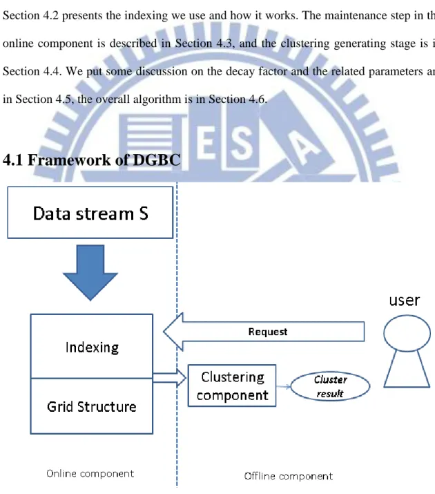
In this chapter, we propose Dynamic Grid-Based Clustering (DGBC), a clustering algorithm based on dynamic grid. Section 4.1 is the framework of DGBC. Section 4.2 presents the indexing we use and how it works. The maintenance step in the online component is described in Section 4.3, and the clustering generating stage is in Section 4.4. We put some discussion on the decay factor and the related parameters are in Section 4.5, the overall algorithm is in Section 4.6.
4.1 Framework of DGBC
20
We overview the overall architecture of DGBC. DGBC is an algorithm with fading model. Like in CLUStream, our method has online and offline components. The online component processes the incoming data and keeps the data summary, and the offline component generates clustering result whenever a user sends a request, as shown in Fig 4.1. The grid structure and the cluster are defined in Chapter 3, and more details are described in the following sections.
4.2 Indexing
Grids are created and deleted during the process as we use dynamic grid structure, so we cannot access them directly. To reduce the time cost on searching, here we propose two types of indexing. One is based on R+ tree, and the other is based on dimensional interval.
4.2.1 R+ Tree-Based Indexing
In an R+ tree based indexing, a node records a grid and the number of data had mapped into it. When a new grid is created, we insert into grid and into the tree.
When a new data arrives, we start from the root node and search if any entry can accept it. If any entry node does, we go down and repeat the process until there is no entries that the data can fit in or the data can accepted by a grid in the leaf level. If the incoming data falls in an existing grid, we simply insert the data into the grid and maintain the grid’s feature vector.
In other case, there is no existing grid for the incoming data, which happens when the incoming data belongs to a new cluster. We have to create a new grid for it
21
because we do not know if it is just an outlier or it is a start of a new cluster. A new grid then is created, taking the current data as the center, and the grid is inserted into the R+ tree, at the last node we search in. The new inserted grid is in the leaf level, and has a pointer to the last searched node. This allows us not need to update all the nodes in the path, saving the updating time when building the index.
(a) (b)
(c) (d)
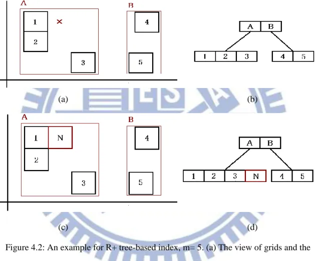
Figure 4.2: An example for R+ tree-based index, m= 5. (a) The view of grids and the arrived data. (b) The index structure when the new data arrives. (c) The view of grids
after the new data is inserted (d) The index structure after the data is inserted.
Fig.4.2 is an example for search and insert a new data on two dimension domain, where m, the capability, is 5. The cross is the incoming data, 1 to 5 is the existing grid, and A, B are the intermediate nodes. When a new data comes in, first we
22
search it from the root node, in which there are two entries, A and B. It belongs to A because it falls in the boundary of A in every dimension. Then we search the child nodes under A. there is no grid that the data can fall into, so we create and insert a new grid, named N, into the tree structure. Fig.4.2 (c) and (d) are the results after the insertion.
R+ trees are good in handling high dimensional data, but sometime they need extra processing time due to the ordering and outliers. A bust of noises may cause several split operations, and the depth of trees are increases. After that, even the noises are cleaned, the search path is longer than before and more time cost is needed to find the data.
4.2.2 Dimensional Interval-Based Indexing
Another type of indexing we use is based on dimensional intervals. For each dimension, we keep an interval list that holds all grids intervals on this dimension. An interval list keeps all grids’ intervals on its dimension in a sorting order. When a new data is coming, we choose a dimension and do a binary search on the interval list to find if the data can fit in any existing grids’ interval. If so, we pour out the grids that do not match in the preview step, choose another dimension and repeat the process until there are no grids. If there are no existing grids that the data can be mapped into, we create a new grid, take the incoming data as the grid center and insert the data. Then we update the interval list on every dimension. Any time if an interval contains no grid, the interval will be deleted. This only happens right after a grid is deleted, so it needs only to update or maintain the list when any grid is deleted.
23
(a) (b)
(c) (d)
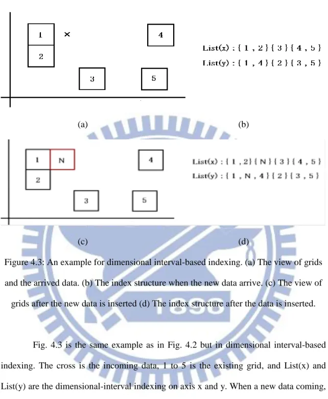
Figure 4.3: An example for dimensional interval-based indexing. (a) The view of grids and the arrived data. (b) The index structure when the new data arrive. (c) The view of
grids after the new data is inserted (d) The index structure after the data is inserted.
Fig. 4.3 is the same example as in Fig. 4.2 but in dimensional interval-based indexing. The cross is the incoming data, 1 to 5 is the existing grid, and List(x) and List(y) are the dimensional-interval indexing on axis x and y. When a new data coming, first we search it from the x-dimension list, the grids in the list are 1 and 2. Then we search the y-dimension list and the there is no interval for the new data. We can know that there must be no existing grid which can accept the data because the intersections of the search results are empty. The algorithm then creates a new grid, named N, for the data and updates the grids list in every dimension. Fig.4.3 (c) and (d) are the result after
24
the data insertion.
When there are d dimensions, we need to keep d lists and may have to search in all lists to discover the target grid. However in most of the cases, after doing search on several dimensions, there are only a few grids remaining, so we can just check them and find out the result we want. This happens more often especially in the high dimension data. When the dimension increases, usually the data are being sparse except at the cluster cores. We can get the target grid in checking only a few dimensions, hence it still works well even for high dimensional data.
4.3 Maintenance Step and Grid Resizing
For every time period, we maintain the grid structure. In the maintenance step, three parts need to be done: maintain grids, update index if needed, and resize the grids.
First, the sparse grids will be removed at the regulating step. A grid with too low density means that it may be a noise or outlier, or it was a high dense unit far time ago and is not meaningful anymore. As we use dynamic grid structure, this can also control the number of grids in use and reduces the memory usage and time cost. When a grid is deleted in this way, the passed information will be lost, so we have to make sure that if a grid is safe to be deleted. We will make a discussion in the later section to show that we can choose a suitable time gap to do it effectively without losing too much of the data information, and also show that this is a necessary operation to keep the data storage bounded.
If any grid is deleted in this way, then the algorithm also needs to update the indexing if needed. For each deleted grid, the algorithm will check and update the index, the node and entry in R+ tree, or its dimensional interval on every dimension. If the
25
deleted grid is the last object in the R+ tree node or interval, the corresponding index structure will also be deleted.
In a dimensional interval based-indexing, this can be done by simply check if the interval contains no object and should be removed at the same time. In an R+ tree-based index, first we remove the grid node, and then check if there are still any other objects under its parent node. If not, the parent node is also deleted, and repeat the process until the root node or a node that still has other objects. There is no need to reinsert the object in the deleted entry node, since R+ tree does not require node to be half filled. In a data stream, there is no information about the data property, so it is hard to find a good parameter setting for every time point. As using a dynamic grid structure, we can adjust the grid size according to the recent data distribution. We keep a global data feature vector to record the information.
Definition 13 (Data feature vector)
The data feature vector is denoted as Dv = { 𝐴̅, 𝑆 ⃑⃑⃑⃑⃑ , 𝑆𝑆 ⃑⃑⃑⃑⃑ } where 𝐴̅ is the number of data in recent time stamp,
𝑆
⃑⃑⃑⃑⃑ is a d-dimension vector that stores the linear sum of data in each dimension for the recent 𝐴̅ data, and
𝑆𝑆
⃑⃑⃑⃑⃑ is a d-dimension vector that stores the square sum of data in each dimension for the recent 𝐴̅ data.
By the data feature vector, the recent 𝐴̅ data’s distribution can be found and computed from the information that is kept. We can resize the grid with the information kept in the data feature vector. Some method resized the grid by merging or reset the distance boundary, but the grid size or maximum boundary may continuously grow and
26
turn into a very large grid. A large grid may takes more data then others, losing meaning and the clustering information. So we have to make sure that out method can work well under the condition.
Definition 14 (Grid Resizing)
The algorithm assigns new grid boundary after the maintenance step. Let 𝐵(T+1) denote the new grid boundary on the 𝑖𝑡ℎ dimension at time T+1, and 𝐵(T) denote the boundary currently used for the 𝑖𝑡ℎ dimension.
The new grid size on the 𝑖𝑡ℎ dimension is computed by
𝐵(T+1) = 𝑅𝑎 𝑆𝑡(T, T+1) (8)
where Ra is a constant of ratio factor for the grid size, and
𝑆𝑡(T, T+1) is the root-mean-square deviations based on recent 𝐴̅ data arrived between T and T+1
From Eq. (8), it clearly shows that the grid boundary at any time point is bounded between [0, Ra*St]. As we resize the boundary depended on the data feature and not the information stored in grids, the boundary can be expanded and reduced over time. For a noisy data, we can update Eq. (8) by adding a weight factor to St and the old boundary. This can provide a smooth changing boundary between the time stamps.
4.4 Cluster Generation
At any time, a user can send a request and the offline component generates clustering results from the online structure. First we find out all high dense grids, and generate clusters by connecting them into grid groups as in Def. 11. Just like the method
27
in DUC-Stream [10], we treat the grid structure as a graph. The vertexes are the grids and there is an edge between two grids if they are neighbor. A depth first search is used to merge grids and generate grid clusters.
The indexing can also reduce the merging time in generating clusters. By Def. 8 and Def. 9, usually we need to check all grids and find their neighbors, then to decide to merge them or not. When the number of dimensions and the number of grids increases, the time cost also increases not only because more objects need to be processed, but also there are more possible neighbors to check. By the index, we can partition all grids into unconnected sets. Only grids in the same set need to be checked because grids in different sets are impossible to be neighboring.
In an R+ tree-based index, we check the nodes from the root, merge the connected nodes and repeat to the child nodes they contain. In a dimensional interval-based index, we choose a dimension and split it into unconnected parts, then choose another dimension and repeat the process in each part. After the partition, we check and merge the neighboring grids in the sets and generate the result, the cluster label and the grids’ information with the same label.
4.5 Decay Factor, Threshold, and Time gap
The algorithm maintains the grids and index structure to control the number of grids and index by removing the spare grids. Some measures can help make a suitable choice.
We define the data rate of a stream as Rx, the high threshold is Dh, the low threshold is Ds, and the decay factor is λ. We can find a good setting that can handle the grid and index structure effectively.
28
Lemma 2 (Grow Gap, TH)
The grow gap, denoted as TH, is the minimum time needed for a sparse grid to become a high dense grid.
TH = λ ℎ λ λ (9)
Proof:
A grid G is a sparse grid at time , by Def. 6, (G, ) ≤ Dw,
If G becomes a high dense grid at time , let 𝐶 (x), 𝐶 (x) …𝐶 (x) denote the sets of data that are inserted into G between time 1 to , and C(x) = ⋃𝑞∈[ ]𝐶𝑞 x , if G becomes a high dense grid at time , by Def. 5,
(G, ) ≥ Dh
(G, ) = ∑ ∈ x + (G, ) * λ
= ∑ ∈ x + (G, ) * λ = ∑𝐶𝑞 x ∈ x ∑ ∈𝐶𝑞 x + (G, ) * λ We know that (G, ) ≤ Ds, and since 𝐶 (x), 𝐶 (x) …𝐶 (x) ≤ Rx,
(G, ) ≤ λ * Rx+ 𝜆 * Rx+ 𝜆 * Rx+ ...+ 𝜆 * Rx + Ds* λ Therefore, λ ≥ ℎ λ λ , δ ≥ λ ℎ λ λ . (10)
By Eq. (10), the minimum time for a spare grid to become a high dense grid is
29
Lemma 3 (Decay Gap, TS)
The decay gap, denoted as TS, is the minimum time needed for a high dense grid to become a sparse dense grid.
TS = λ ℎ (12)
Proof:
A grid G that is a high dense grid at time , by Def. 5, (G, ) ≥ Dh
If G becomes a sparse grid at time , let C(x) denotes the sets of data that are inserted into G between time 1 to , we want that G become a sparse grid at time ,
(G, ) = ∑X∈ x + (G, ) * λ ≤ Dw, We know that C(x) ≥ 0 , we have
(G, ) ≤ (G, ) * λ ≤ Dw, Therefore
λ ≥ ℎ , λ ℎ (13) By Eq(13), the minimum time for a high dense grid to become a sparse grid is
TS = λ ℎ (14)
Lemma 4 (Living Gap, TM)
The living gap, denoted as TM, is the minimum time needed for an empty grid to become an intermediate grid.
TM = λ λ 1 . (15)
30
An empty grid G is a grid with no data inserted before time (G, ) = 0
If G becomes an intermediate grid at time , let 𝐶 (x), 𝐶 (x) …𝐶 (x) denotes the sets of data that are inserted into G between time 1 to , and C(x) = ⋃𝑞∈[ ]𝐶𝑞 x ,, we want that G becomes a high dense grid at time , by Def.7,
(G, ) ≥ Dw
(G, ) = ∑ ∈ x + (G, ) * λ
= ∑𝐶𝑞 x ∈ x ∑ ∈𝐶𝑞 x + (G, ) * λ We know that (G, ) = 0, and since 𝐶 (x), 𝐶 (x) …𝐶 (x) ≤ Rx,
(G, ) ≤ 𝜆 * Rx+ 𝜆 * Rx+ 𝜆 * Rx+ ...+ 𝜆 * Rx
λ ≥ λ
1, δ ≥ λ
λ
1 . (16)
By Eq(16), the minimum time for an empty grid to become an intermediate grid is
TM = λ λ 1 (17)
Now we can decide the time gap, the period that the algorithm should check and maintain the structure, from the above result.
The time gap we choose should not be too small. If we maintain the structure every time when a new data comes, it will lead to a heavy overhead and slow down the system. Also, most of the data information will be removed because we remove sparse grids in the maintenance stage. Many of the grids do not receive enough data and are deleted before they can reach the low threshold and become an intermediate grid.
31
may be lost. The cluster features may change obviously during a large time gap. Some of the clusters may show up and then disappear in the time gap. So the time gap we choose need to be small enough to discover the change of cluster features. For an intermediate node, we want to catch the changes that it becomes a high dense grid, or becomes a sparse grid and be removed by the algorithm. Also if we choose a too large time gap, the system will have to keep more grids and indexing information. These storages will increase the search time since they increase the size of index and the number of grids.
Definition 15 (Time Gap, TG)
The Time gap, denoted as TG, defines how often we check and maintain the grids and index structure.
TM< TG < Min (TS, TH) (18)
Another measure is to show how our method can work under a bounded memory. Since the data stream is infinite, we need to limit the storage usage.
Lemma 5 (The Maximum Density, MD)
The maximum density, denoted as MD, is the sum of density coefficients from all data. It is bounded by
MD ≤
(19)
Proof:
Given a time T, Md = ∑ ∈T is the total density coefficient during the time 0 to T 𝐶 (x), 𝐶 (x) …𝐶T(x) denote the sets of data arrived at time 0,1,2 …, T. 𝐶 (x), 𝐶 (x) …𝐶T(x) ≤ Rx, and C(x) = ⋃𝑞∈[ T]𝐶𝑞 x
32
∑ ∈ x = ∑𝐶𝑞 x ∈ x ∑ ∈𝐶𝑞 x
≤ 𝜆 * Rx+ 𝜆 * Rx+ 𝜆 * Rx+ ... +𝜆 * Rx
∑ ∈T ≤ o 𝜆 * Rx+ 𝜆 * Rx+ 𝜆 * Rx+ ... +𝜆 * Rx
= Rx * (20) Therefore, from Eq(20),
MD = ∑ ∈ x ≤ (21)
A living grid is a grid that needs to keep after the maintenance step. It is a high dense grid or an intermediate grid. Since the maximum data density kept is bounded, we know that the number of living grids is also bounded. And at any time point, the total number of grids we need is also bounded by the number of living grids and the data rate.
Lemma 6 (Maximum Living Grid, MA)
The maximum living grid, denoted as MA, is the maximum number of the sum of intermediate grids and high density grids. MA is the number of grids that needs to keep after any maintenance step.
MA ≤ (22)
Proof:
From Eq. (19), we know that at any time point, that maximum density coefficient from all data records is no more than MD. After the maintenance step, all grids whose density lower than Ds will be removed, so all the living grids have density at least Dw. Therefore, the maximum number of living grids is .
33
Definition 13 (Maximum Grid, MG)
The number of maximum grids in use, denoted as MG, is the maximum number of all the grids in the algorithm at any time.
MG ≤ 𝑅 (23) The worst case shows up when a time point contains only noise or all of the incoming data belong to a different grid. The case is rare in the real data streams, and most of the grids will be deleted at next maintenance step.
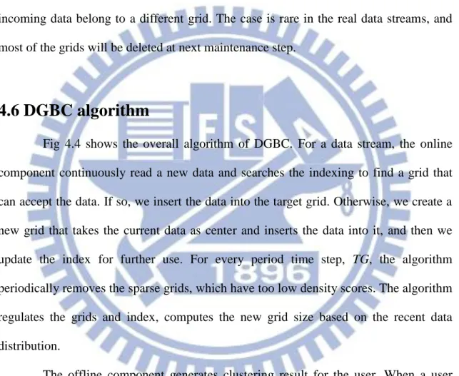
4.6 DGBC algorithm
Fig 4.4 shows the overall algorithm of DGBC. For a data stream, the online component continuously read a new data and searches the indexing to find a grid that can accept the data. If so, we insert the data into the target grid. Otherwise, we create a new grid that takes the current data as center and inserts the data into it, and then we update the index for further use. For every period time step, TG, the algorithm periodically removes the sparse grids, which have too low density scores. The algorithm regulates the grids and index, computes the new grid size based on the recent data distribution.
The offline component generates clustering result for the user. When a user requests, the algorithm finds out all the high density grids, where their density score is higher than the threshold. Then the system tries to merge the neighboring high density grids together and assigns a cluster label for them.
34
Input: data stream S
Output: (Cluster label, grid list)
Variable: time_gap TG, grid ratio R, high threshold Dh, low threshold Dw Initialize:
Current time tc= 0; An empty grid list Glist, index I, ; Data feature vector Dv= 0, Initial grid size B(0).
While data stream is active:
Read data record X= { , …, }. Target_grid = Search (Glist)
if(Target_grid = NULL) Create a new grid Gn.
I.insert(Gn). Target_grid = Gn. endif Target_grid.insert(X). Updata Dv. if( tc == time_gap TG)
for all grid G in Glist
if( G.density < Dw )
remove G from Glist. Update I. else
Decay G.density. Compute new grid size B(tc)=𝑅 𝑆𝑡
endif
When requested:
An empty grid list Gh. for all grid G
if G.density > Dh.
Gh.insert(G)
endif
Return cluster_result = generate_cluster(Gh)
35
Chapter.5
Experimental Results
We compare our method with CLUStream, DUC-Stream, D-stream, AGD-stream and IGDLC. Two types of index are used, represent as DGBC(DI) and DGBC(R+). The CLUStream algorithm is based on distance factor and the others are based on density. All algorithms were implemented in C++ language and tested on an i7-2600k 3.4 GHz with 16G memory running Microsoft Windows 7 Professional system. The comprehensive performance study has been conducted on both synthetic and real world datasets. To show the efficiency of DGBC, we perform three kinds of experiments. First, we compare the execution time and clustering quality of DGBC with other streaming clustering algorithms using synthetic datasets. Second, we investigate the scalability of DGBC. Finally, we apply DGBC in some real datasets to compare the performance and also discuss the effect of initial setting.
5.1 Clustering Quality
The clustering quality is measured by clustering purity. Purity is a simple and transparent evaluation measure. To compute purity, each cluster is assigned to the class which is most frequent in the cluster, and then the accuracy of this assignment is measured by counting the number of correctly assigned members and divided by the total number of members in this cluster. Eq. (25) shows the purity in one cluster, and Eq(24) is the total purity from all clusters.
36
Purity (𝐶) = |𝐶
𝑗| |𝑛 𝑚𝑏𝑒𝑟 𝑓 𝑚𝑎𝑗 𝑟 𝑖𝑡𝑒𝑚 𝑖𝑛 𝐶| (25)
where k is the number of clusters, N is the total number of data recorded.
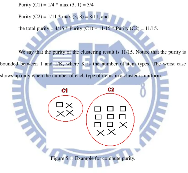
For example, we generate two clusters as in Fig.5.1. There are two different types of item in each group. By Eq(24) and Eq(25), the purity in each cluster are
Purity (C1) = 1/4 * max (3, 1) = 3/4
Purity (C2) = 1/11 * max (3, 8) = 8/11, and
the total purity = 4/15 * Purity (C1) + 11/15 * Purity (C2) = 11/15.
We say that the purity of the clustering result is 11/15. Notice that the purity is bounded between 1 and 1/K, where K is the number of item types. The worst case shows up only when the number of each type of items in a cluster is uniform.
Figure 5.1: Example for compute purity.
5.2 Data Generator
The synthetic data sets in the experiments are generated using synthetic generation program proposed by Vennam et al. [18]. The parameter setting of data generator is shown in Table 1.
37
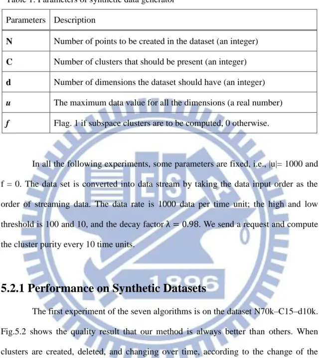
Table 1: Parameters of synthetic data generator Parameters Description
N Number of points to be created in the dataset (an integer)
C Number of clusters that should be present (an integer)
d Number of dimensions the dataset should have (an integer)
u The maximum data value for all the dimensions (a real number)
f Flag. 1 if subspace clusters are to be computed, 0 otherwise.
In all the following experiments, some parameters are fixed, i.e., |u|= 1000 and f = 0. The data set is converted into data stream by taking the data input order as the order of streaming data. The data rate is 1000 data per time unit; the high and low threshold is 100 and 10, and the decay factor λ 0.98. We send a request and compute the cluster purity every 10 time units.
5.2.1 Performance on Synthetic Datasets
The first experiment of the seven algorithms is on the dataset N70k–C15–d10k. Fig.5.2 shows the quality result that our method is always better than others. When clusters are created, deleted, and changing over time, according to the change of the data property, the algorithm adjusts the generated and existing grids periodically, so it is able to capture the evolution of the data stream and generates high quality clustering result.
38
Figure 5.2: Quality comparison (Synthetic dataset N70k–C15–d10k)
Fig.5.3 shows the result of execution time. CLUStream needs the most time because it needs a linear search on all micro-clusters for the insertion. IRGC also needs a search on all grids, so when the number of grids increases over the process, the search cost increases. At the start of the process, our method needs some time to set up the index, after that it works effectively as the indexing provides a fast search and merge operation. 0.8 0.82 0.84 0.86 0.88 0.9 0.92 0.94 0.96 0.98 1 10 20 30 40 50 60 70 P u ri ty Time unit D-Stream AGD-Stream CLU-Stream DUC-Stream IGDLC DGBC(R+ , DI)
39
Figure 5.3: Execution time comparison (Synthetic dataset N70k–C15–d10k)
5.2.2 Scalability Study
In this section, we study the scalability of the DGBC algorithm. Then we test the scalability with the synthetic datasets. We compare between two types of indexing we proposed. The first series of datasets are generated by varying the dimensionality from 10 to 100, while fixing the stream size (100k, the lower lines, and 1000k, the upper lines) and the number of natural clusters (10). Fig.5.4 shows that the execution time of our method is closest to linear with respect to the number of dimensions.
An R+-tree-based index ignored the number of dimensions, so it is ideal to deal with high dimension data. However, it has a high time cost to maintain and update the tree structure especially when the data property changes or the condition is noisy. In these cases, some of the old grids need to be deleted and many new grids are created as new core of clusters or noises, which leads to a heavy overhead since the R+ tree indexing may need several node split operations.
0 0.5 1 1.5 2 2.5 3 3.5 4 4.5 10 20 30 40 50 60 70 E xc u tio n t im e (s ec) Time unit D-Stream AGD-Stream CLU-Stream DUC-Stream IGDLC DGBC(DI) DGBC(R+)
40
When the number of dimensions increases, the dimensional interval-based index needs to keep more information for each dimension, but the search time and merge time increases slowly as in higher dimension, the data become sparser. In the usual case, we can find the grids within checking a few dimensions, and do not really need to check on all dimensions to find the target grid.
Figure 5.4: Scalability test with different number of dimensions. (Synthetic datasets)
The other series of datasets are generated by varying the number of natural clusters from 2 to 50, while fixing the stream size (100k, the lower lines, and 1000k, the upper lines) and the number of dimensions (10). Fig.5.5 shows that the execution time of our method is stable with respect to the number of clusters. When the number of cluster increases, we need to be more careful not to merge data belonging to different cluster together. The two scalability tests can show that our method is suitable for both high dimensional data and dispersive data.
0 50 100 150 200 250 10 20 30 40 50 60 70 80 90 100 E xc u tio n t im e( se c) Number of dimensions R+ (1000K) DI (1000K) R+ (100K) DI (100K)
41
Figure 5.5: Scalability test with different number of clusters. (Synthetic datasets)
5.3 Network Intrusion Detection dataset
The KDD-CUP’99 Network Intrusion Detection dataset [27] consists of raw TCP connection records from a local area network. Each record in the dataset corresponds to either a normal connection or an attack. There are four attack types: DOS (denial of service), R2L (unauthorized access from a remote machine, e.g., guessing password), U2R (unauthorized access to root), and PROBING (surveillance and other probing). As a result, the data contains five clusters including the class label of normal, and the attack types are further classified into 24 types. Most of the connections in this dataset are normal, but sometimes there may have burst of attacks at certain times. The cluster property evolves significantly over time. We use the type of connection as its cluster label. As in other experiments [4] [6], all 34 out of the total 42 continuous attributes available are used for clustering. The data rate is 1000 data per time unit; the high and low threshold, Dh and Dw, is 100 and 10, and the decay
0 10 20 30 40 50 60 70 80 90 100 2 6 10 14 18 22 26 30 34 38 50 E xc u tio n t im e( se c) Number of cluster R+ (1000K) DI (1000K) R+ (100K) DI (100K)
42
factor λ 0.98. We send a request and compute the cluster purity every 10 time units.
5.3.1 Performance on Network Intrusion Detection dataset
Fig.5.6 is the result of clustering quality. It shows that our proposed method usually better than others. For all algorithms, the quality of clustering falls when the cluster property changes, but our proposed method can adapt itself to catch the new data property. Especially in a dataset that is noisy and evolves significantly during process as in the Network Intrusion dataset, our method performs much better to find and generate meaningful results. Our method works well on the Charitable Donation dataset even it has less noises and the cluster property is stable.
Figure 5.6: Quality comparison (Network Intrusion dataset)
Fig. 5.7 shows the result of execution time. CLUStream spend most of the time cost because it needs to do a liner search on all micro-clusters for the insertion for every
0.7 0.75 0.8 0.85 0.9 0.95 1 P u ri ty Time unit D-Stream AGD-Stream CLU-Stream DUC-Stream IGDLC DGBC(R+ , DI)