液晶排列配向結構之動態取影與逆問題

國立交通大學

電機資訊學院

顯示科技研究所

碩士論文

液晶排列配向結構之動態取影與逆問題

Dynamic Optical Probing and Inverses Problem of Liquid Crystal

Alignment Structures

研究生：李建輝

指導教授：黃中垚 教授

液晶排列配向結構之動態取影與逆問題

Dynamic Optical Probing and Inverses Problem of Liquid Crystal

Alignment Structures

研究生：李建輝

Student：Jien-Hui Li

指導教授：黃中垚

Advisors：Professor Jung Y. Huang

國立交通大學電機資訊學院

顯示科技研究所

碩士論文

A Thesis

Submitted to Institute of Display

College of Electrical Engineer and Computer Science

National Chiao Tung University

in Partitial Fulfillment of the Requirements

for the Degree of

Master

in

Display Institute

September 2008

Hsinchu, Taiwan, Republic of China

液晶排列配向結構之動態取影與逆問題

研究生：李建輝 指導教授：黃中垚 教授

國立交通大學

顯示科技研究所

摘要

液晶的排列指向在液晶應用是很重要的性質。在本篇論文中，我們利

用加入混合垂直配向的延展態液晶盒做為例，以模擬計算與量測的光

學結果相比較，得到靜態與動態液晶指向分佈資訊。我們模擬計算液

晶的排列與光學反應使用液晶自由能張量表現型式。實驗量測使用高

靈敏度攝影機搭配延遲時間產生器來擷取液晶盒的動態影像。我們針

對取得液晶的排列指向逆問題做了理論分析與實驗示範。結果發現在

加入混合垂直配向可消除延展態液晶的暖機時間，但也增加了液晶盒

的反應時間。在利用逆問題的方法取得液晶的排列指向，我們提出了

符合液晶特性的正則化矩陣，並驗證使用大範圍入射角的光學測量數

據和系統量測誤差在百分之十下，在此逆問題求解是穩定而可靠的。

從實際實驗示範成功展示在不同施加電壓下的液晶盒內之液晶排列

指向可穩定而可靠取得。

Dynamic Optical Probing and Inverses Problem of Liquid

Crystal Alignment Structures

Student：Jien-Hui Li Advisors：Professor Jung Y. Huang

Department of Photonics and Display Institute,

National Chiao Tung University

Abstract

The liquid crystal (LC) director profile is an important property for a variety of LC applications. In this study, we combine simulation and experimental measurement of the optical responses of hybrid alignment liquid crystal cells to demonstrate the functionality of LC director profile retrieval. Our simulation invokes the Q-tensor formalism of liquid crystal director calculation and Berreman matrix method for the optical response of LC. An electron-multiplying charge coupled device and a delay time generator were combined to capture the dynamic optical image of the liquid crystal cells. We discovered that by including a hybrid alignment region into an OCB cell, the warm up time of the LC cell can be effectively eliminated. The relaxation time was unfortunately also increased. We also study the inverse problem of LC to retrieve the director profile of liquid crystal cell directly from the measured optical transmittance data. To retrieve the director profile from the inverse problem technique, we proposed a regularization matrix based on a priori knowledge of LC. We found our method can yield LC director profile reliably from the measured optical data covering a wide range of incident angle and 10% noise level. We further demonstrated the functionality by retrieving the liquid crystal director profiles of LC cells with applied voltage from the experimentally measured data.

誌謝

在碩士班的時間裡，感謝指導教授 黃中垚教授所給予我偌大的

收穫，讓我真正體會到做一份研究所需要的嚴謹態度以及用邏輯的思

考來解決問題。雖然過程辛苦，但是我想唯有紮實的訓練，才是真正

做學問的基礎。

再來感謝實驗室裡的柳萱學姐，總是能給我適當的協助與解答，

還有雲漢學長、秉寬學長、燦丞、綿綿、建佑，給了在嚴肅的研究生

活裡最好的調劑。

最後要感謝的是我的父母與家人，提供我精神上最大的支持，讓

我能夠用最積極的狀態來完成這份研究。

Content

Abstract (in Chinese) i

Abstract (in English) ii

Acknowledgement (in Chinese) iii

Contents iv

List of Tables vi

List of Figures vii

1

Introduction to the Physical and Optical Properties of LC 1

1.1 Motivation...2

1.2 The Physics of Liquid Crystal...3

1.3 The Optical Properties of Liquid Crystal...7

2

Models of the LC Alignment Structure and the Optical Response

12

2.1 The Q-Tensor Formalism...13

2.2 The Berreman Matrix Method...21

2.3 The Application Examples...30

3

Dynamic Optical Probing for Hybrid Alignment Liquid Crystal

Cells 38

3.2 The Modification of The Existing OCB Cell………..39

3.3 Experimental Setup of the Dynamic Optical Probing

Apparatus...41

3.4 Results and Discussion…………...43

4

Inverse Problem of Liquid Crystal Director Profile 56

4.1 Introduction to the Inverse Problem...56

4.2 The Inverse Problem of Liquid Crystal Director Profile...62

4.3 Theoretical Details...65

4.4 Simulation Results and Discussion...71

5

Inverse Retrieval of Liquid Crystal Director Profile from

Measured Optical Transmittance Data 81

5.1 Experimental Apparatus for Inverse Problem Retrieval...81

5.2 Experiment Results and Discussion...82

6

Conclusions and Future Prospect of This Thesis Study 92

List of Tables

2-1 The material parameters of LC used for the simulation...33

3-1 The LC cell and material parameters used in this experiment...42

3-2 The response times of each cells are given...45

3-3 The optical images of the two line-patterned cells at different delay times...48

4-1 Comparison of the calculation results with the two different methods based on Eq. (4.25) and Eq. (4.26). Eq. (4.26) is calculated to the fourth order of Taylor expansion...73

List of Figures

1-1 (a) Different shapes of liquid crystal molecules. (b) The molecular alignments in the SmC, SmA, and the nematic phases...1 1-2 An example to describe nematic LC with an averaged molecular direction

picture...3 1-3 Two cases of the distribution function of molecular orientation θ_mwith (a) high

orientational order, (b) low orientational order...4 1-4 Three kinds of deformation commonly existing in a liquid crystal medium...6 1-5 A diagram showing ordinary and extraordinary rays in a LC medium...8 1-6 Schematic showing the way to generate on and off state with a positive Δε LC

material...9 1-7 Shcematic showing two kinds of LC alignment: (a) planar, (b) hybrid...11 2-1 An optical beam incidents on a homogeneous anisotropic layer at an angleϕ₀..23 2-2 Schematic showing the coordinates system and a stratified anisotropic medium

between two isotropic media...26 2-3 The flowchart of the simulation used to calculate the alignment configuration

and optical response of nematic LC...32 2-4 The simulation structure with a square of defect. (a) The mesh plot. ( b) The plot

of simulation result...34 2-5 (a) The schematic showing the distribution of LC pretilt angle from the bottom to the top plate. (b) The pretilt angle distribution of a LC cell with different anchoring energies...35 2-6 The simulation results revealing the influence of the separation of in-plane

electrodes on LC alignment...36 2-7 The calculated optical transmittance of a LC cell, which has both a homeotropic

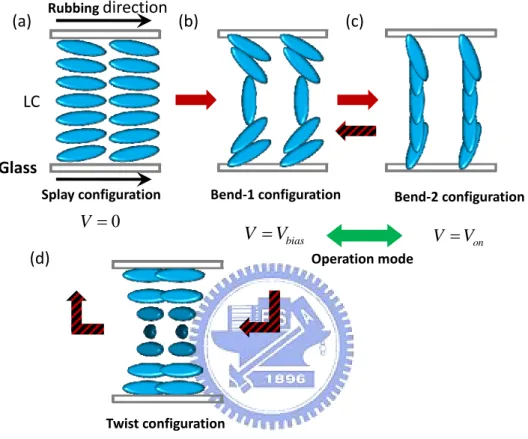
and hybrid alignment zones inside, and the pretilt angle distribution are plotted...37 3-1 The geometric transition of the OCB cell as applied voltage. (a) Splay

configuration. (b) Bend 1 configuration. (c) Bend 2 configuration. (d) Twist configuration...39 3-2 The schematic and the side view of our modified OCB cell...41 3-3 (a) The setup of dynamic optical probing comprising of a delay generator to

control the time delay. (b) The waveform and the trigger signal applied on the sample and the EMCCD...43 3-4 Optical response curves of four different LC cells (homogeneous OCB,

homogeneous hybrid, and 2 mμ - and 4 mμ -line patterned hybrid OCB cells....44 3-5 The optical transmittance is measured after the applied voltage is removed. The

measurement results reveal the LC twist motion in each cells...45 3-6 The optical micrographic images of the line-patterned hybrid cells. The

resolution of the microscope is about 0.3 mμ ...46 3-7 (a) The measured and calculated optical transmittance images of two

line-patterned LC hybrid alignment cells in a region covering one period ( 90 mμ ). (b) The measured and the simulated optical transmittance images of the4 mμ -line patterned cell and the gray level profiles horizontally cut through

the images at the center of the vertical position...47 3-8 The summed gray-level value over a region covering one period in each image of

Table 3-3 is plotted as a function of delay time...49 3-9 The optical transmittance (in terms of gray-level ) of the 2 mμ and 4 mμ -line

patterned cells was measured under a crossed polarizer-analyzer. The summed gray-level values over the region with hybrid alignment configuration (Hybrid) and over the region with OCB splay configuration (Splay) are plotted as a

function of delay time...50 3-10 The measured optical transmittance (in terms of gray-level) of the 2 mμ and

4 mμ -line patterned cells is plotted as a function of delay time. The direction of the polarizer is aligned with the rubbing direction and the analyzer is set to cross with the polarizer...52 3-11 The calculated optical transmittance variation (in terms of gray-level change) of

a TN cell with a twist angle varying from 0D to 180D. Two TN cells with cell gaps 4 and 10 μm were used for the simulation...52 3-12 The calculated director profile and optical transmittance of the 4 mμ line-patterned cell at delay time of5ms, 15ms, 25ms and 75ms...53 3-13 The measured and simulated optical transmittance variation (in terms of

gray-level change) is plotted as a function of delay time. The 4 mμ line-patterned cell was inserted between a cross polarizer-analyzer with (a) the direction of the polarizer aligning to the rubbing direction, (b) the direction of the polarizer deviating from the rubbing direction by1.82D...54 4-1 (a) The Stability distribution of x . (b) The Stability distribution of b...60 4-2 The L-curve is a curve in a log-log scale with λIx 2 on the y-axis and

2

Ax - b on the x-axis by varying λ from 10−5 to 1. The optimal value of λ is be chosen is at the corner of the curve labeled with the red circle...62 4-3 The schematic showing the setup implemented to collect the data with various

incident angles of light...63 4-4 (a) Schematic showing the difference between our new approach and the HP

group’s method. (b) The flowchart of searching for the LC director profile with optical transmittance data...65 4-5 The experimental setup used to measure the optical transmittance data for

inverse problem retrieval of LC director profile...72 4-6 The schematic showing an idea that decomposes a LC cell into several layers to

facilitate the calculation of optical transmittance...73 4-7 Comparison of the retrieved LC director profiles by using different regularization methods. The transmittance data are prepared first with the finite element simulation based on Q-tensor approach and then added with one percentage of noise. (a) LC director profile retrieval by using one-constant regularization parameter λ . (b) LC director profile retrieval by using our new regularization scheme...74 4-8 LC director profiles retrieved with the transmittance data. The data are prepared

first with the finite element simulation based on Q-tensor approach and then added with 1%, 5%, 10%, 15%, 20%, 30% of noise. (a) The retrieved LC director profiles. (b) The statistics of the total deviation of the profiles to the true solution...78 4-9 The retrieved LC director profiles with the three ranges of simulated optical

transmittance data: I (+10 ~ 10D − D), II(+30 ~ 30D − D), and III( 50 ~ 50+ D − D)....79 5-1 The experimental setup used to measure the optical transmittance data for

inverse problem retrieval of LC director profile...81 5-2 The polarization-resolved optical transmittance measurement results T and _x T _y

of the LC cell with hybrid alignment are presented by using four different input polarization states (22.5o, 67.5o, 112.5o, and CP). The LC cell was applied with 0V. Two curves are included for comparison: red open squares: simulated curve with Berreman matrix technique, and blue cross symbols: the measured transmittance as a function of optical incident angle...84 5-3 The polarization-resolved optical transmittance measurement results T and _x T _y

of the LC cell with hybrid alignment are presented by using four different input polarization states (22.5o, 67.5o, 112.5o, and CP). The LC cell was applied with 2.5V. Two curves are included for comparison: red open squares: simulated curve with Berreman matrix technique, and blue cross symbols: the measured transmittance as a function of optical incident angle...85 5-4 The polarization-resolved optical transmittance measurement results T and _x T _y

of the LC cell with hybrid alignment are presented by using four different input polarization states (22.5o, 67.5o, 112.5o, and CP). The LC cell was applied with 5V. Two curves are included for comparison: red open squares: simulated curve with Berreman matrix technique, and blue cross symbols: the measured transmittance as a function of optical incident angle...86 5-5 The polarization-resolved optical transmittance measurement results T and _x T _y

the OCB cell with bend-splay alignment are presented by using four different input polarization states (22.5o, 67.5o, 112.5o, and CP). The LC cell was applied with 0V. Two curves are included for comparison: red open squares: simulated curve with Berreman matrix technique, and blue cross symbols: the measured transmittance as a function of optical incident angle...87 5-6 The polarization-resolved optical transmittance measurement results T and _x T _y

the OCB cell with bend-splay alignment are presented by using four different input polarization states (22.5o, 67.5o, 112.5o, and CP). The LC cell was applied with 2.5V. Two curves are included for comparison: red open squares: simulated curve with Berreman matrix technique, and blue cross symbols: the measured transmittance as a function of optical incident angle...88 5-7 The polarization-resolved optical transmittance measurement results T and _x T _y

the OCB cell with bend-splay alignment are presented by using four different input polarization states (22.5o, 67.5o, 112.5o, and CP). The LC cell was applied with 5V. Two curves are included for comparison: red open squares: simulated curve with Berreman matrix technique, and blue cross symbols: the measured transmittance as a function of optical incident angle...89 5-8 The retrieval director profiles of the hybrid cell by inverse problem method. (a)

The coordinate system used to present the LC director profiles. (b) The retrieved director profiles of the hybrid cell biased at 0V, 2.5V, and 5V. Two profiles are included for comparison: red squares: retrieved profile, and blue symbols: the simulated profile calculated by the FEM with Q-tensor approach...90 5-9 The retrieval director profiles of the OCB cell by inverse problem method. (a)

The coordinate system used to present the LC director profiles. (b) The retrieved director profiles of the OCB cell biased at 0V, 2.5V, and 5V. Two profiles are included for comparison: red squares: retrieved profile, and blue symbols: the simulated profile calculated by the FEM with Q-tensor approach...91 6-1 An example of the iterative regularization method with different iteration

number……….94 6-2 Optical microscope with high NA objective can be used to simplify the data

taking procedure for inverse problem retrieval. (a) The experiment setup. (b) The NA value of the objective lens for our incident angle range………96

Chapter 1

Thesis Motivation and the Introduction to the

Physical and Optical Properties of LC

Liquid Crystal (LC) is an intermediate state of a matter between the isotropic liquid and the crystal. In the LC state, several phases with different molecular alignment orders can be found. LC molecules have typical shapes of rod-like, discotic-like, and bend-shape. Figure 1-1 illustrates the different phases and shapes of LC molecules. For simplicity of this thesis study, we will focus only on the rod-like LC molecules in the nematic phase. [1]

Figure 1-1 (a) Different shapes of liquid crystal molecules. (b) The molecular

n

K

Nematic phase  Smectic A phase 

n

K

n

K

ˆz

θ

Smectic C phase  Temperature 

n

K

n

K

n

K

(a)    (b) 

1.1 Motivation

Liquid crystal display (LCD) has been widely used in the flat panel display (FLD) industry. To satisfy the ever-increasing need for information flow and display, the next generation LC display will demand accurate control of LC configuration in each LC pixels. The static and dynamic alignment structures of liquid crystal molecules are important factors for the optical properties and response of a LC device. To probe the response of a LC device, a variety of optical techniques can be used to yield useful insight. However, the optical data are usually resulted from the entire liquid crystal layer along the propagation direction of the optical beam used. To offer the detailed information of LC director profiles and allow for the further progress of LC devices, we developed in this thesis two techniques to retrieve the LC director profiles of LC devices. We termed the first approach with a name of the model extraction. The method iteratively compares the simulation result with the measured data and retrieves the LC director profile. The second method invokes the inverse problem technique by way of optical transmittance measurement of a LC device and retrieving the LC director profile directly from the measured data. We demonstrate these two methods as in Chapters 3 and 4. However, to fulfill the objective, in the flowing we will first depict the physical and optical properties of LC materials in chapter 1 and

then in chapter 2 illustrate the models developed to simulate the LC alignment structure and the resulting optical response.

1.2 The Physics of Liquid Crystal

A rigid rod-shaped molecule is the simplest picture to be used for the description of the nematic LC. For an elongated molecule, the alignment status and the positions of the centers of mass of the molecules determine the state of matter. We can first define the averaged molecular orientation of a nematic LC, which is called director

(

nK

)

, as shown in Figure 1-2.

Figure 1-2. An example to describe nematic LC with an averaged molecular direction picture.

Because the director is an averaged vector over a small local volume, we need to further specify how the LC molecules angularly spread about the direction. A convenient measure of the amount of order is the scalar order parameter, denoted by

θ m

θ

m

θ

−

n

K

LC molecules 

molecular axes and the director. Eq. (1.1) describes how to calculate the scalar order parameter: 2 1 3cos 1 2 m S = θ − , (1.1)

where denotes the thermal or statistical average. Therefore, Eq. (1.1) can be rewritten as:

(

2

)

( )

1 3cos 1 2 B m m S =

∫

θ − f θ dV , (1.2)

where B denotes the volume of integration and f

( )

θ is the distribution function _m

of the molecular angle θ_m. Figure 1-3 presents two cases of the distribution function

(

m

f θ with a high and a low orientational order. As we can see in the Figure 1-3,

)

because of the symmetry of molecule, f

( )

θ shall be even with _m f

( )

θ_m = f

(

−θ_m

)

and periodic f

(

θ_m+π

)

= f

( )

θ_{m . We can easily calculate a perfect crystal to have}

and for an isotropic fluid.

1

S= S =0

( )

m

f θ f

( )

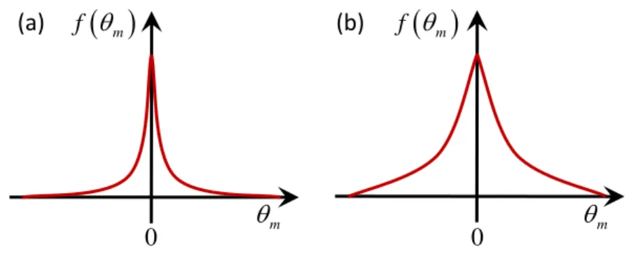
θ_m

(a)  (b) 

Figure 1-3 Two cases of the distribution function of molecular orientation

m

θ with (a) high orientational order, (b) low orientational order.

According to the Frank-Oseen theory, the Gibbs free energy density of a nematic

m

θ θm

LC medium can be expressed as

(

)

(

)

(

)

(

)

(

)

(

)

(

)

(

)

(

)

2 2 11 22 33 22 24 0 22 2 0 1 1 1 2 2 2 1 2 1 2 1 , 2

G elastic electric surface

f f f f K n K n n K n n K K n n n n q K n n D E W n n 2 = + + = ∇ ⋅ + ⋅∇× + ×∇× ⎡ ⎤ − + ∇ ⋅_⎣ ∇ ⋅ + × ∇× _⎦ − ⋅∇× − ⋅ + − K K K K K K K K K K K K K K K (1.3)

by taking the elastic, the electric and the surface energy density into account. Each term can be explained as follows:

The expression at the first line, which describes the elastic deformation energy of the LC medium, is comprised of three terms representing the most important elastic distortion energies in LC: splay

(

K₁₁

(

∇⋅ Kn

)

2

)

, twist

(

K₂₂

(

nK⋅∇×nK

)

2

)

24

K

, and bend with three corresponding elastic constants. at the second line is related to the surface anchoring energy and at the third line is the chirality of the LC. Figure 1-4 shows the LC molecular alignment with the three different elastic deformations. In fact, the elastic constants in a typical LC material are very small in the order of pN, implying that LC material is quite easy to be influenced by an external force field.

(

(

2 33 K nK×∇×nK

)

)

0 q

Splay  Twist  Bend 

Figure 1-4. Three kinds of deformation commonly existing in a liquid crystal medium.

The expression at the fourth line describes how the LC molecules interact with an electric field. This is the foundation of LC applications. For LC with dielectric constants, ε_& (parallel to the molecular long axis) and ε_⊥ (perpendicular to the molecular long axis), we can relate the electric energy to the LC director by using el f _ectric

(

)

(

0

)

1 2 1 , 2 electric f D E V V ε ε = − ⋅ = − ∇ ⋅∇ K K I (1.4)

where ε is the dielectric tensor of LC, and can be conveniently expressed as I

ij ij n ni j

ε =ε δ_⊥ +Δε

(

i j, =x y z, ,

)

, with Δ = −ε ε ε_{& ⊥} and δ the Kronecker delta, _ij which is 1 if i equals j, and 0 otherwise.

The expression at the fifth line is the surface energy or called surface anchoring energy, where nK₀ denotes the prefer alignment direction of LC molecules on surface

and is the surface anchoring strength. A useful model of surface anchoring energy is Rapini-Papoular form [2].

W

In a physical system, the equilibrium stable state tends to have a structure with minimum free energy. Thus, we can use this property to calculate the director configuration by minimizing the free energy density of LC. We can use the functional minimization technique to yield the result that the target functionals shall satisfy the Euler-Lagrange equations: , , , , , , 0, and 0, G G G G i i x i y i z G G G G x y z f d f d f d f dn dx dn dy dn dz dn f d f d f d f dV dx dV dy dV dz dV ⎛ ⎞ ⎛ ⎞ ⎛ ⎞ ∂ ₋ ∂ ₋ ∂ ₋ ∂ ₌ ⎜ ⎟ ⎜ ⎟ ⎜ ⎟ ⎜ ⎟ ⎜ ⎟ ⎜ ⎟ ⎝ ⎠ ⎝ ⎠ ⎝ ⎠ ⎛ ⎞ ⎛ ⎞ ⎛ ⎞ ∂ ∂ ∂ ∂ − ⎜_⎜ ⎟_⎟− ⎜_⎜ ⎟_⎟− ⎜_⎜ ⎟_⎟= ⎝ ⎠ ⎝ ⎠ ⎝ ⎠ (1.5)

where f is the Gibbs free energy density describing by Eq. (1.3). _G

1.3 The Optical Properties of Liquid Crystal

LC has been widely used in fat panel display industry due to its attractive visco-elastic and electro-optical characteristics. To reveal its unique properties, we will study in this section the electro-optical behavior of LC under an electric field.

Nematic LC is an optical uniaxial medium with birefringence characterizing by two principal refractive indices. The refractive index, which is given by n c

υ = , is inverse proportional to the velocity of light, υ, traveling in the medium, and c

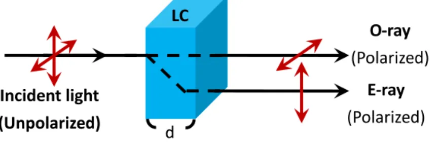
nematic LC film, it would experience two different velocities inside the LC, which we called ordinary-ray and extraordinary-ray. Therefore, a phase retardation will be experienced between the o-ray and e-ray in the LC film. Figure 1-5 illustrates how we can convert a unpolarized light into a polarized light by using a LC cell.

d LC  (Polarized)  E‐ray  (Polarized)  O‐ray  (Unpolarized)  Incident light 

Figure 1-5 A diagram showing ordinary and extraordinary rays in a LC medium.

We can introduce ordinary and extraordinary refractive indices and birefringence as:

, ,_&

o e e

n = ε_⊥ n = ε Δ =n n − . (1.6) n_o

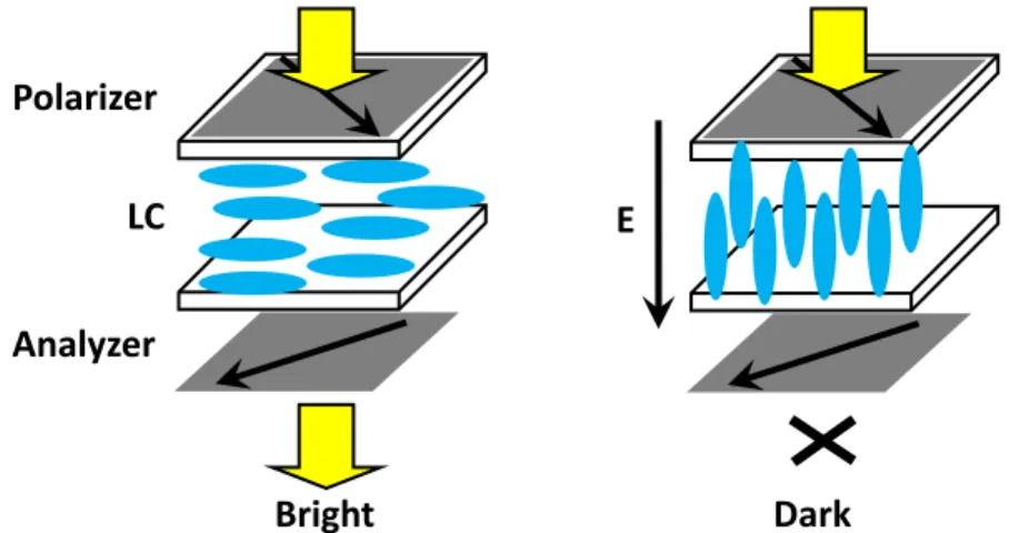
From Eq. (1.4) and Eq. (1.6), we found that the dielectric constants and refractive indexes can be affected by electric field. Figure 1-6 describes a general operational principle of LC applications.

E LC  Dark Bright  Polarizer  Analyzer 

Figure 1-6. Schematic showing the way to generate on and off state with a positive Δε LC material.

The propagation of a polarized optical beam in a LC cell can be properly described with Jones matix formalism [3]. For an analysis, we first introduce a coordinate system with x- and y-axis lying on the plane of the LC cell. A Jones vector is used to describe the state of polarization of light with a complex envelope that represents the amplitude and phase of the optical field:

(1.7) 0 0 . x y i x x i y _y V e V V _{V e} ϕ ϕ ⎛ ⎞ ⎛ ⎞ ⎜ =_{⎜ ⎟ ⎜}= ⎝ ⎠ ⎝ ⎠ V ⎟ ⎟

The resulting intensity is given by:

2 2 * . x y I =VV =V +V (1.8)

By the description, we can construct a Jones matrix to connect the incoming and the outgoing wave in a vector form:

(1.9) 11 12 21 22 , J J J J ⎛ ⎞ = _{= ⎜ ⎟} ⎝ ⎠ out in in V JV V

refractive indices and , inserted between crossed polarizers. By taking into account the optical axis of the LC cell relative to the laboratory frame, we can derive an expression for the system in Jones matrix representation:

1

n n₂

( )

ϕ

( )

ϕ , = y − slab x in

V_out P R J R P V (1.10)

where P_i

(

i=x,y

)

denotes the polarizer, R

( )

ϕ is the rotation matrix, and ϕ is

the angle of the optical axis of the birefringent slab relative to the x-axis of the laboratory frame. By substituting each matrix into Eq. (1.10), the result becomes:

( )

( )

(

)

1 1 2 2 1 2 0 0 c si 0 cos sin 1 0 0 1 sin cos sin cos 0 0

0 . sin 2 i n d out in x x out i in n d y y i in x V e V V V e n n d iV e π λ π λ π λ ϕ ϕ ϕ ϕ π λ − − − + ⎛ ⎞ ⎛ ⎞₌⎛ − ⎜ ⎟⎛ ⎞⎛ ⎞⎛ ⎞ ⎜ ⎟ ⎜ _{⎜ ⎟}⎜ ⎟⎜ ⎟⎜ ⎟ ⎜ ⎟ _{⎝ ⎝− ⎠⎝ ⎠}⎜ ⎟ ⎝ ⎠ ⎜ ⎟ ⎝ ⎠ ⎝ ⎠ ⎛ ⎞ ⎜ ⎟ =_⎜ ⎛ − ⎞_⎟ ⎜ ⎟ ⎜ _{⎝ ⎠}⎟ ⎝ ⎠ 1 2 os n n d ⎞ ⎟ ⎠ n 0 sin ϕ ϕ ϕ ϕ ϕ ⎛ ⎞ ⎜ ⎟ ⎝ ⎠ . (1.11)

From Eq. (1.8) and Eq. (1.11), we can further obtain the output light intensity:

(

)

( )

( )

( )

( )

(

)

1 2 2 2 2 1 2 2 _{2 2 1 2} sin 2 sin sin . x y i n n in x in x I V V n n d iV e n n d V π λ _ϕ π λ π λ − + = + ⎛ − ⎞ = _{⎜ ⎟} ⎝ ⎠ ⎛ − ⎞ = _{⎜ ⎟} ⎝ ⎠ sin 2 d ϕ . (1.12)

Eq. (1.12) is useful to analyze the light propagation through a LC slab (Figure 1-7(a)). For a planar aligned LC with a pretilt angle θ with respect to the cell surface, the optical plane wave traveling through the LC cell will experience an effective refractive index of

        2 2 2 2 . sin cos e o eff e o n n n n θ n θ = +        (1.13)  By substituting n₁=n_eff and n₂ = into Eq. (1.12), it becomes: n_o

( )

2 ₂

( )

₂ 2 2 2 2 sin 2 sin . sin cos in e o x o e o n n d I V n n n π ϕ λ _{θ θ} ⎛ ⎛ ⎞⎞ ⎜ ⎜ ⎟⎟ = − ⎜ ⎟ ⎜ _{⎝ + ⎠}⎟ ⎝ ⎠ (1.14)

For a hybrid LC cell (see Figure 1.7(b)) with a LC director profile a linear variation of distance, we can derive the output light intensity to be

( )

( )

( )

( )

2 _{2 2} 2 2 2 2 0 sin 2 sin . sin cos d in e o x o e o n n I V dz dn n z n z π ϕ λ _{θ θ} ⎛ ⎛ ⎞⎞ ⎜ ⎜ ⎟⎟ = − ⎜ ⎜ ₊ ⎟⎟ ⎝ ⎠ ⎝

∫

⎠ (1.15) (a)  Hybrid  Planar  (b) 

Figure 1-7. Shcematic showing two kinds of LC alignment: (a) planar, (b) hybrid.

Chapter 2

Models of the LC Alignment Structure and the

Optical Response

Over the past several years, liquid crystal has been widely used for information display applications. As the technology becomes more and more sophisticated, computer simulation on LC devices becomes more important. Simulation can help researchers probing into the static and dynamic behaviors of LC and the optical properties thereafter. By calculating the director configuration and optical response of LC, we can predict what kinds of defects might develop and what optical responses could be yielded. To compute the director profile, it is required to express the free energy density of LC as shown in Eq. (1.3). By minimizing the free energy density, the LC alignment configuration can be obtained.

We found in Eq. (1.3) that it does not include the order parameter, , which is one of the important parameters of nematic LC. By including the order parameter into the free energy density, the defect formation can be described with the solution in a more intuitive way. In addition, we also discover that Eq. (1.3) is in the vector representation. The free energy density expression may have different values for

S

S

and −n [4]. However, for a real nematic LC, n and − shall be equivalent and n

possess the same free energy based on the symmetry argument. By using the Landau-de Gennes’s Q-tensor representation of free energies [5, 6] to calculate the LC director configuration, the above-mentioned difficulty can be avoided. The equivalence between the Frank-Oseen’s vector representation and Landau-de Gennes’s Q-tensor representation has been proved by Dickman [7].

Once we have retrieved the director profile of a nematic LC, we can analyze its optical response to reveal more useful information for its application properties. In the chapter 1, we have introduced the Jones matrix method which is a powerful tool to analyze the optical properties of a layer-stacked medium at normal incidence. But to calculate the optical properties of a layer-stacked medium at high incident angle with multiple reflections, the Jones matrix method does not give a precise result. For this reason, we choose the Berreman 4 4× matrix method [8], which is based on the assumption of plane wave propagation in a stratified medium.

2.1 The Q-Tensor Formalism

Consider the 3 3× matrix,

(

n

)

,

S n

= ⊗

M K K (2.1)

mathematical operation on the director vector nK=

(

n n n_x, _y, _z

)

with the rule (2.2) . x y x z y y y z z y z z n n n n n n n n n n n n ⎛ ⎞ ⎜ ⎟ ⎜ ⎜ ⎟ ⎝ ⎠ x x y x z x n n n n n n n n ⊗ = K K ⎟ 1 nK =

We note that the director vector is an unit vector with and this makes the trace of to be . The other property of the matrix is the symmetric property. We can then define Q-tensor as

M S M 1 , 3 S n⎛ n = _⎜ ⊗ − ⎝ ⎠ Q K K I⎞_⎟ (2.3)

which is symmetric and traceless. With the definition, we can derive the Q-tensor formalism of free energy from the Frank-Oseen free energy density.

We first define some elastic free energy density parameters, corresponding to each terms present in Eq. (1.3):

2 1 2 2 2 3 4 5 ( ) ( ) ( ) [ ( ) ( )] F F F F F = ∇ ⋅ = ⋅∇× = ×∇× = ∇ ⋅ ∇ ⋅ + × ∇× = ⋅∇× n n n n n n n n n n n K K K K K K K K K K K (2.4)

and then construct the following vectors:

1 2 3 4 5 33 11 22 22 24 0 22 [ , , , , ] [ , , , , ] 2 2 2 2 T T F F F F F K K K K K q K = + = − − F F K . (2.5)

By using Eq. (2.4) and Eq. (2.5), we can rewrite the elastic free energy density in an inner product of row and column matrices by

.

elastic

In the next step, some convenient parameters, which are bilinear forms of the elastic free energy density parameters defined in Eq. (2.4), can be defined

( )

2

1 j j, , 2 j k, j k, , 3 j k l j, j k, , 4 j k, k j, , 5 j l k, jkl,

f = n f =n n f =n n n n f =n n f =n n e (2.7) where Einstein summation convention is invokes, e_jkl is the Levi-Civita symbol

defined by and all other , and

is defined as:

1, 1,

xyz yzx zxy xzy yxz zyx

e =e =e = e =e =e = − ejkl =0 nj k,

{

, , , , , . j j k n n j k x k y z

}

∂ = ∈ ∂ (2.8)

We prepared a vector f that possesses the components of Eq. (2.7):

[

1, 2, 3, 4, 5

]

.

T

f f f f f

=

f (2.9)

The relationship between the two vectors F and can be found f

(2.10) , F = Af with 1 0 0 0 0 0 1 1 1 0 . 0 0 1 0 0 1 0 0 1 0 0 0 0 0 1 ⎡ ⎤ ⎢ _{− −} ⎥ ⎢ ⎥ ⎢ ⎥ = ⎢ ₋ ⎥ ⎢ ⎥ ⎢ ⎥ ⎣ ⎦ A (2.11)

After the necessary preparation, the elastic free energy density in Eq. (1.3) can be expressed as a linear combination of the vector f and an elastic constant vector K_f:

(2.12)

.

s

f =K F = K Af = K fTF TF f T

33 22 11 22 24 22 24 0 22 , , , , 2 2 2 2 T K K K K K K K q K − − − ⎡ ⎤ =_⎢ − _⎥ ⎣ ⎦ T f F K = A K . (2.13)

We can define bilinear Q-tensor terms by using the same approach detailed in Eq.

(2.7): 1 , , 2 , , 3 , , 4 , 5 , , , , , , and jk l jk l jk k jl l jk l jl k jkl jm km l jk lm j lm k G Q Q G Q Q G Q Q G e Q Q G Q Q Q = = = = = (2.14) where 3 jk jk j k Q =S n n⎛_⎜ −δ ⎞_{⎟ jk}

⎝ ⎠, δ is Kronecker’s delta, and is the scalar order parameter. We then define a vector in terms of the bilinear Q-tensor components as:

S 3 5 1 2 4 2, 2 , 2 , 2 , 3 T G G G G G S S S S S . ⎡ ⎤ = ⎢_⎣ ⎥_⎦ g (2.15)

The relationship between f and is now clear to be g

g = Bf (2.16) with 0 2 0 0 0 1 0 1 0 0 2 . 2 1 1 0 3 0 0 0 0 1 0 1 3 0 0 ⎡ ⎤ ⎢ ⎥ ⎢ ⎥ ⎢ ⎥ = ⎢ ⎥ ⎢ ⎥ − ⎢ ⎥ ⎢ ₋ ⎥ ⎣ ⎦ B (2.17)

By defining a new elastic constant vector for vector g , the elastic free energy density can be rewritten as:

g K

.

s

f =K g = K Bf = K BA FT_g T_g T_g -1 (2.18) Comparing Eq. (2.6), Eq. (2.12) and Eq. (2.18), we obtain

-T T -T g F

K = B A K = B K_f -1

(2.19) where . By using Eq. (2.13) and Eq. (2.17), we can also find

that

( ) ( )

T -T -1 T B = B = B

(

)

(

)

(

)

33 11 22 11 22 24 24 0 22 33 11 1 3 12 1 3 2 1 2 1 6 K K K K K K K q K K K ⎡ _{− +} ⎤ ⎢ ⎥ ⎢ ⎥ ⎢ _{− −} ⎥ ⎢ ⎥ ⎢ ⎥ = ⎢ ⎥ ⎢ ⎥ ⎢ ⎥ ⎢ ⎥ ⎢ ₋ ⎥ ⎢ ⎥ ⎣ ⎦ T g K (2.20)

Finally, by substituting Eq. (2.15) and Eq. (2.20) into Eq. (2.18), the Q tensor representation of the elastic free energy density becomes

(

)

(

)

(

)

3 1 2 33 11 22 2 11 22 24 2 24 5 4 0 22 2 33 11 3 1 1 3 3 12 2 2 1 6 s G G G f K K K K K K K S S G G q K K K S S = − + + − − + + + − 2 1 S (2.21)

To include the electric free energy density of Eq. (1.4) into Eq. (2.21), we can express it in terms of the Q-tensor representation by following the Einstein summation convention

2 0 , , , , 1 , 2 2 , 3 , . jk electric j j k j Q f V V V S V V j ε ε ε ε ε ε ε ε ε ⊥ ⊥ ⎛ ⎞ = _⎜ + Δ _⎟ ⎝ ⎠ + = Δ = − ∂ = ∂ & & (2.22)

For the surface free energy density, the Q-tensor representation is

(

2 2 , 2 surface s W f S = Q Q− _s

)

(2.23)

where S is the preferred surface order parameter. Thus, by combining Eq. (2.21), Eq. _s

(2.22), and Eq. (2.23) together, we finally obtain the Euler-Lagrange equation in the

Q-tensor representation , , , , , , 0, and 0. G G G G jk jk x jk y jk z G G G G x y z f d f d f d f dQ dx dQ dy dQ dz dQ f d f d f d f dV dx dV dy dV dz dV ⎛ ⎞ ⎛ ⎞ ⎛ ⎞ ∂ ∂ ∂ ∂ − ⎜_⎜ ⎟_⎟− ⎜_⎜ ⎟_⎟− ⎜_⎜ ⎟_⎟ ⎝ ⎠ ⎝ ⎠ ⎝ ⎠ ⎛ ⎞ ⎛ ⎞ ⎛ ⎞ ∂ ∂ ∂ ∂ − ⎜_⎜ ⎟_⎟− ⎜_⎜ ⎟_⎟− ⎜_⎜ ⎟_⎟= ⎝ ⎠ ⎝ ⎠ ⎝ ⎠ = (2.24)

We can calculate the director profile of LC with the Q-tensor formalism. For example, by solving the eigen-modes of Eq. (2.24) we can produce the static LC director profiles for our LC design. The LC dynamic response is also an important issue for LC application. By using Erickson-Leslie theory and neglecting the inertial momentum of LC molecules, the dynamic visco-elastic behaviors of nematic LC can be analyzed with a modified version of Eq. (2.24) shown below

, , , , , , 0, jk G G G G jk jk x jk y jk z G G G G x y z Q f d f d f d f t dQ dx dQ dy dQ dz dQ f d f d f d f dV dx dV dy dV dz dV γ ∂ = −_⎜⎜⎛ ∂ − ⎛⎜_⎜ ∂ ⎞_⎟⎟− _⎜⎛⎜ ∂ ⎟_⎟⎞− ⎜⎛_⎜ ∂ ⎟⎞_⎟⎟⎞_⎟ ∂ _{⎝ ⎝ ⎠ ⎝ ⎠ ⎝ ⎠⎠} ⎛ ⎞ ⎛ ⎞ ⎛ ⎞ ∂ ∂ ∂ ∂ − ⎜_⎜ ⎟_⎟− ⎜_⎜ ⎟_⎟− ⎜_⎜ ⎟_⎟= ⎝ ⎠ ⎝ ⎠ ⎝ ⎠ , (2.25)

where γ denotes the rotational viscosity of nematic LC.

We examined Q tensor in Eq. (2.3) and found that it meets the following two criteria: zero trace ( _ii 0) and a unit vector (

i Q =

∑

_ii 1 i n =

∑

) of LC director. Based on our experience of calculating the director profile under an electric field, we often encountered that our solution cannot converge and LC director is not a unit vector during iteration. These difficulties had also been reported in literature [9]. Therefore, to solve Eq. (2.25), the conditions of zero trace ( _ii 0

i

Q =

∑

) and a unit vector ( ) of LC must be maintained at each time step. To meet the traceless condition, we renew the diagonal terms of Q tensor with the replacing scheme

1 ii i n =

∑

( )

. 3 new old ii ii Trace Q =Q − old Q (2.26)

For the normalization condition of LC director, it can be implemented simply as:

2 2 2 . old new i i x y z n n n n n = + + (2.27)

( )

2 2 2 2 2 2 2 2 2 '( ) 1 '( ) ( ) ' '( ) '( 1) ' ' ( ). ' i j new ij x y z i j x y z i j x y z old n n Q S n n n S n n n n n S S n n S n n n S S Q S Trace = + + = × + + = × + + − + = + _Qold (2.28)

For the diagonal components of Q tensor, the following normalization conditions can be used 2 2 2 2 2 2 2 2 2 2 2 2 2 2 2 2 2 2 2 2 2 2 2 2 2 2 2 2 2 2 1 '( ) 3 '( ) 3( ) 1 '( ) 3 ( ) ( 1) 1 ' '( ) 3 3 '( 1) ' ( 1 ( '( ) ' 3 new i ii x y z x y z i x y z x y z x y z i x y z x y z i x y z x i n Q S n n n n n n n S n n n n n n n n n S n n n n n n n S S n S n n n S n S n S = − + + + + = − + + + + + + = − × + + + + − = − − × + + − + + = − −

( )

( )

2 2 2 2 2 1) ' ) 3 '( 1 ' ( )( ). 3 ' y z x y z old n n S S n n n S Trace _S Q S Trace + − × ) ' + + − + = − + old old Q Q (2.29)

The in Eq. (2.28) and Eq. (2.29) is not the same value as we use at the beginning of simulation. To illustrate this problem, let us take a look at the Q tensor at the beginning:

'

1 ( ) ( ) ( ) 3 1 ( ) ( ) ( ) 3 1 ( ) ( ) ( ) 3 x x x y x z y x y y y z z x z y z z S n n S n n S n n S n n S n n S n n S n n S n n S n n ⎡ ₋ ⎤ ⎢ ⎥ ⎢ ⎥ ⎢ ⎥ =_⎢ − _⎥ ⎢ ⎥ ⎢ ₋ ⎥ ⎢ ⎥ ⎣ ⎦ Q . (2.30)

It is clear that Eq. (2.30) has the following eigenvalues

2 2 2 [ 3 ( )] 2 . 3 3 3 3 3 3 x y z S S n n n S S S S S λ= −⎡⎢ − − + + + ⎤_{⎥ ⎢}= −⎡ − ⎤_⎥ ⎣ ⎦ ⎢ ⎥ ⎣ ⎦ (2.31)

The new ' therefore shall be evaluated with the eigenvalues of instead of using the initial value at the beginning.

S Qold

2.2 The Berreman Matrix Method

Based on the Maxwell’s equations

, , 0, and 0, t t ∂ ∇× = − ∂ ∂ ∇× = − ∂ ∇ ⋅ = ∇ ⋅ = B E D H B D (2.32)

we can describe the wave propagation in a layered medium in a matrix formalism. This can be done by expressing curl and divergence operation as a matrix

0 0 , 0 z y . x z x y x _z ∂ ∂ ⎛ ⎞ ⎛ ⎞ y ∂ − ⎜ _{∂ ∂} ⎟ ⎜_∂ ⎟ ⎜ ⎟ ⎜ ⎟ ∂ ∂ ⎜ ⎟ ⎜ ⎟ ∇× =_⎜ − _⎟ ∇⋅ =_{⎜ ⎟} ∂ ∂ ⎜ _{∂ ∂} ⎟ ⎜ ⎟ ⎜ ⎟ ∂ ∂ ∂ ⎜ ⎟ − _{⎜ ⎟} ⎜ _{∂ ∂} ⎟ _{⎝∂ ⎠} ⎝ ⎠ (2.33)

components can be properly described as follows: 0 0 0 0 0 0 0 0 0 0 0 0 . 0 0 0 0 0 0 0 0 0 0 0 0 x y x y _z z x x y y z z D z y _t D E z x _t E _D E y x _t H B z y H t B H t z x B t y x ∂ ∂ ⎛ ₋ ⎞ _{⎛∂ ⎞} ⎜ _{∂ ∂} ⎟ _{⎜ ⎟} ∂ ⎜ ⎟ _{⎜ ⎟} ∂ ∂ ⎜ ₋ ⎟ _⎜∂ _⎟ ⎜ _{∂ ∂ ⎟⎛ ⎞ ⎜ ⎟} ∂ ⎜ _{⎟⎜ ⎟ ⎜ ⎟} ∂ ∂ ⎜ ₋ ⎟⎜ ⎟ ⎜∂ ⎟ ⎜ ∂ ∂ _⎟⎜ ⎟ ⎜ _∂ ⎟ ⎜ _{∂ ∂} ⎜ ⎟ ⎜= _∂ ⎜ _{− ⎟⎜ ⎟ ⎜ ⎟} ⎜ _{∂ ∂ ⎟⎜ ⎟ ⎜ ∂ ⎟} ⎜ _{⎟⎜⎜ ⎟ ⎜⎟ ∂ ⎟} ∂ ∂ ⎜_{− ⎟⎝ ⎠ ⎜ ⎟} ⎜ _{∂ ∂} ⎟ _{⎜ ∂ ⎟} ⎜ ⎟ _{⎜∂ ⎟} ∂ ∂ ⎜ ₋ ⎟ _{⎜ ⎟} ⎜ _{∂ ∂} ⎟ _{⎝ ∂ ⎠} ⎝ ⎠ ⎟ _{⎟ (2.34)}

Eq. (2.34) can be expressed in a matrix form as: . t ∂ = ∂ C OG (2.35)

In the absence of spatial dispersion and nonlinear optical effects, the constitutive relations D=ε₀εE and B=μ₀μH can be easily included in Eq. (2.34). For simplicity, we use time harmonic optical fields, in which the ei tω factor can be taken out of the field components. Under the condition, Eq. (2.35) can be simplified as:

( )

(

)

, , and , i t i t t e i e i ω _ω ω ω ∂ ∂ = G OG = M O Γ = M Γ OΓ MΓ (2.36) where 0 11 0 12 0 13 0 21 0 22 0 23 0 31 0 32 0 33 0 11 0 12 0 13 0 21 0 22 0 23 0 31 0 32 0 33 0 0 0 0 0 0 0 0 0 0 0 0 0 0 0 0 0 0 ε ε ε ε ε ε ε ε ε ε ε ε ε ε ε ε ε ε μ μ μ μ μ μ μ μ μ μ μ μ μ μ μ μ μ μ ⎛ ⎞ ⎜ ⎟ ⎜ ⎟ ⎜ ⎟ = ⎜ ⎟ ⎜ ⎟ ⎜ ⎟ ⎜ ⎟ ⎜ ⎟ ⎝ ⎠

of G.

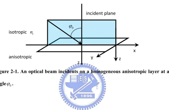
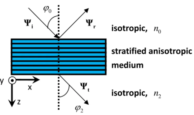
As shown in Figure 2-1, we consider a monochromatic plane wave obliquely incident from an isotropic medium to a homogeneous anisotropic layer medium with the surface normal along the z-axis.

z y z x 0 ϕ incident plane  anisotropic  isotropic  n_i 

Figure 2-1. An optical beam incidents on a homogeneous anisotropic layer at an angleϕ₀.

The problem is invariant along the y-direction, so all derivatives along y can be set to zero

0.

y

∂ ₌

∂ (2.37)

The incident plane wave E=E e₀ i(ωt−kr) must have the same spatial dependence on x. The x-component of the wave vector k in the ambient medium of index _x n_i is:

0 isin ,

k n ₀

ξ = ϕ (2.38)

where ϕ₀ is the angle of incidence and k₀ c

ω

= . The variation of all fields in the x-direction is proportional to e−i xξ , so we can get:

.

i x ξ

∂ _{= −}

∂ (2.39)

We assume that the magnetic permeability of a nematic LC is isotropic and the dielectric permittivity tensor can be related to the pretilt and azimuthal angle of the LC director by μ 2 2 2 2 2 2 2 2 2 2 0 0 0 0 , and 0 0

cos cos cos sin cos sin cos cos

cos sin cos cos sin sin cos sin

sin cos cos sin cos sin sin

o o o n n n μ μ μ ε θ φ ε θ φ φ ε θ θ φ ε θ φ φ ε θ φ ε θ θ φ ε θ θ φ ε θ θ φ ε θ ⎛ ⎞ ⎜ ⎟ = ⎜ ⎟ ⎜ ⎟ ⎝ ⎠ ⎛ + Δ Δ Δ ⎞ ⎜ ⎟ = Δ_⎜ + Δ Δ _⎟ ⎜ _{Δ Δ + Δ} ⎟ ⎝ ⎠ μ ε (2.40)

where θ denotes the pretilt angle and φ denotes the azimuthal angle. Combining Eq. (2.38), Eq. (2.39) and Eq. (2.40) into Eq. (2.36), we obtain the wave propagation equations for all field components

0 11 0 12 0 13 0 21 0 22 0 23 0 31 0 32 0 33 0 0 0 0 0 0 0 0 =0 . 0 0 0 0 0 0 0 0 0 0 0 x y z x y z i i i z E i i i i E z i i i i E H i z H H i i z i i ωε ε ωε ε ωε ε ωε ε ωε ε ωε ε ζ ωε ε ωε ε ωε ε ζ ωμ μ ζ ωμ μ ζ ωμ ∂ ⎛ ⎞ ⎜ _∂ ⎟ ⎜ _{⎟⎛ ⎞} ∂ ⎜ _{− −} ⎟_{⎜ ⎟} ⎜ _∂ ⎟_{⎜ ⎟} ⎜ _{⎟⎜ ⎟} ⎜ _{⎟⎜ ⎟} ⎜ _∂ ⎟_{⎜ ⎟} − ⎜ _{∂ ⎟⎜ ⎟} ⎜ _{⎟⎜ ⎟} ⎜ ⎟ ∂ ⎜ _{⎟⎝ ⎠} ⎜ _∂ ⎟ ⎜ ⎟ ⎜ ₋ ⎟ ⎝ μ⎠ (2.41)

The third and the sixth row equations of Eq. (2.41) can be reduced to

31 32 0 33 33 33 0 , and , z y x z y E H E E H E y ε ε ξ ε ε ω ε ε ξ μ μω = − − − = (2.42)

other field components. Replacing E and _z of Eq. (2.41) with of Eq. (2.42), four linear, first-order differential equations for the field components

z

H

x

E , E_y, −H_x(minus sign for convenience and simplicity), and H_yare obtained

2 31 32 0 2 33 0 33 33 0 13 31 13 0 13 32 0 11 ε ε0 12 0 23 33 ξε ω ε ε ε 33 33 33 0 2 0 23 31 23 32 0 21 22 2 33 33 0 0 0 0 0 0 0 x y y x E H E z H i ξε _{μ μ} ξ ωε ω ε ε ε ε ε ε ξε ε ε ε ε ε ω ε ω ε ε ε ξε ε ξ ε ε ε ε ω ε ω μ ⎛ ⎞ ⎜ ⎟ ∂ ⎜ ⎟ ⎜ ⎟ ∂ ⎜₋ ⎟ ⎝ ⎠ − − − − − − = − − − ₀ − − ε ε ε x y y x E H E H ⎛ ⎞ , ⎟ ⎟ ⎟ ⎟ μ μ μ ⎛ ⎞ ⎜ ⎟ ⎜ ⎟ ⎜ _⎟⎜ ⎜ _⎟⎜ ⎜ _⎟⎜ ⎜ _⎟⎜ ⎜ ⎟ −_⎝ ⎜ ⎟ ⎜ ⎟ ⎝ ⎠ ⎠ (2.43) or in a matrix form . i z ω ∂ _{= −} Ψ ∂ ΠΨ Π (2.44) Here denotes the differential propagation matrix. Eq. (2.44) can be solved to

yield an analytic solution of

(

+

)

=

( )

z .

Ψ iwh

e− Π z

z h Ψ (2.45)

This yields a generalized field vector Ψ at +h if Ψ is known at z_{. Here} is a finite propagation distance. For a multilayer structure with a total thickness of

, we obtain h i i d =

∑

h

( )

_d =_e n_... − 2Π2_e−iwh1Π1

( )

_{0 .} out n in iwh − Π Ψ iwh e Ψ (2.46)

medium sandwiched between two isotropic media with indices of refraction and . 0 n 2 n

Figure 2-2. Schematic showing the coordinates system and a stratified anisotropic medium between two isotropic media.

With Fresnel equations, we can get the fields in incidence (i), reflection (r) and transmission (t): 0 0 0 0 0 0 0 2 0 , , and . iy ix iy ix ry rx ry rx ty tx ty tx H H n E E H H n E E H H n E E ε μ ε μ ε μ = = = = = = (2.47)

According to Eq. (2.47), the generalized field vectors in each region can be found to be: i Ψ Ψ_r t Ψ 0 ϕ isotropic,  n0  isotropic,  n2  stratified anisotropic  medium y  x z  2 ϕ

0 0 0 0 0 0 0 0 0 0 0 0 0 0 0 0 2 0 2 0 0 2 2 0 cos , cos cos , and cos cos . cos ix ix iy iy rx rx ry ry tx tx ty ty E E n E E n E E n E E n E E n E E n ϕ ε μ ε ϕ μ ϕ ε μ ε ϕ μ ϕ ε μ ε ϕ μ ⎛ ⎞ ⎜ ⎟ ⎜ ⎟ ⎜ ⎟ ⎜ ⎟ = ⎜ ⎟ ⎜ ⎟ ⎜ ⎟ ⎜ ⎟ ⎝ ⎠ − ⎛ ⎞ ⎜ ⎟ ⎜ ⎟ ⎜ ⎟ ⎜ ⎟ = ⎜ ⎟ ⎜ ⎟ ⎜₋ ⎟ ⎜ ⎟ ⎝ ⎠ ⎛ ⎞ ⎜ ⎟ ⎜ ⎟ ⎜ ⎟ ⎜ ⎟ = ⎜ ⎟ ⎜ ⎟ ⎜ ⎟ ⎜ ⎟ ⎝ ⎠ i r t Ψ Ψ Ψ (2.48)

Thus, Eq. (2.45) can be modified to be

(

)

( ) , P = t i Ψ Π Ψ + Ψ_r (2.49)

where is the propagation matrix. Substituting Eq. (2.48) into Eq. (2.49), we then have: ( ) P Π (2.50) ( ) , 0 0 ix tx iy ty rx ry E E E E P E E ⎛ ⎞ ⎛ ⎞ ⎜ ⎟ ⎜ ⎟ ⎜ ⎟ ⎜ _{⎟ =} ⎜ ⎟ ⎜ ⎟ ⎜ ⎟ ⎜ ⎟ _{⎜ ⎟} ⎝ ⎠ ⎝ ⎠ 2 1 T Π T which results in

(2.51) , 0 0 ix tx iy ty rx ry E E E E E E ⎛ ⎞ ⎛ ⎞ ⎜ ⎟ ⎜ ⎟ ⎜ ⎟ ⎜ _{⎟ =} ⎜ ⎟ ⎜ ⎟ ⎜ ⎟ ⎜ ⎟ _{⎜ ⎟} ⎝ ⎠ ⎝ ⎠ b U with (2.52) ( ) , P = -1 b 2 1 U T Π T where 0 0 0 0 0 0 0 0 0 0 0 0 0 0 0 0 cos 0 cos 0 0 0 , and 0 1 0 1 0 cos 0 cos n n n n ϕ ϕ ε ε μ μ ε ε ϕ ϕ μ μ − ⎛ ⎞ ⎜ ⎟ ⎜ ⎟ ⎜ ⎟ ⎜ ⎟ = ⎜ ⎟ ⎜ ⎟ ⎜ ₋ ⎟ ⎜ ⎟ ⎝ ⎠ 1 T 2 0 2 0 0 2 2 0 cos 0 0 0 0 0 0 0 1 0 0 0 cos 0 0 n n ϕ ε μ ε ϕ μ ⎛ ⎞ ⎜ ⎟ ⎜ ⎟ ⎜ ⎟ ⎜ ⎟ = ⎜ ⎟ ⎜ ⎟ ⎜ ⎟ ⎜ ⎟ ⎝ ⎠ 2 T .

The projection matrices P( )Π can be found to be:

(2.53) 1 0 0 0 0 1 0 0 , and 0 0 0 0 0 0 0 0 0 0 0 0 0 0 0 0 . 0 0 1 0 0 0 0 1 ⎛ ⎞ ⎜ ⎟ ⎜ ⎟ = ⎜ ⎟ ⎜ ⎟ ⎝ ⎠ ⎛ ⎞ ⎜ ⎟ ⎜ ⎟ = ⎜ ⎟ ⎜ ⎟ ⎝ ⎠ + -P P

By using Eq. (2.51) and Eq. (2.53), we can derive the components of transmitted and reflected waves as:

0

0

b

U

ix tx iy ty rx ry

E

E

E

E

E

E

⎛

⎞

⎛

⎞

⎜

⎟

⎜

⎟

⎜

⎟

⎜

_{⎟ =}

⎜

⎜

⎟

⎜

⎟

⎜

⎟

_⎜

_⎟

⎝

⎠

⎝

⎠

⎟

, (2.54) which leads to 0 0 0 0 + b b P U U tx ix ty iy rx rx ry ry E E E E E E E E ⎛ ⎞ ⎛ ⎞ ⎛ ⎞ ⎜ ⎟ ⎜ ⎟ ⎜ ⎟ ⎜ ⎟₌ ⎜ ⎟₊ ⎜ ⎜ ⎟ ⎜ ⎟ ⎜ ⎟ ⎜ ⎟ ⎜ ⎟ ⎜ ⎟ ⎜ ⎟ _{⎝ ⎠} ⎜ ⎟ ⎝ ⎠ ⎝ ⎠ ⎟ ⎟ ⎟ i 4 4× and _. 0 0 tx tx ix ty ty iy rx rx ry ry E E E E E E E E E E ⎛ ⎞ ⎛ ⎞ ⎛ ⎞ ⎜ ⎟ ⎜ ⎟ ⎜ ⎟ ⎜ ⎟₋ ⎜ ⎟₌ ⎜ ⎟ ⎜ ⎟ ⎜ ⎟ ⎜ ⎟ ⎜ ⎟ ⎜ ⎟ ⎜ ⎟ ⎜ ⎟ ⎜ ⎟ _{⎝ ⎠} ⎝ ⎠ ⎝ ⎠ + b - b P U P U

Therefore

(

)

or in the matrix notation simply as

0 0 -1 + b - b P - U P U tx ix ty iy rx ry E E E E E E ⎛ ⎞ ⎛ ⎞ ⎜ ⎟ ⎜ ⎟ ⎜ ⎟₌ ⎜ ⎜ ⎟ ⎜ ⎜ ⎟ ⎜ ⎟ ⎜ ⎟ _{⎝ ⎠} ⎝ ⎠

(

Ψ_t+Ψ_r

)

= ⋅B Ψ_i =

(

P - U P_{+ b -}

)

-1U Ψ_b . (2.55) By using Eq. (2.55), we can calculate the TM and TE components of the transmitted and reflected waves for given incident TM and TE waves.

Although the Berreman matrix method is a fast and powerful method, it is usually difficult to be used to solve a three-dimensional problem, especially when the geometry is complex. We therefore introduce a modified Jones matrix method to analyze the light transmission for a twisted nematic (TN) LC. The theoretical derivation had been reported by the group of Oldano [10] by using a perturbative approach. The transmission matrix of a TN LC cell was found to be

2 * ₂ , a i ik d i e it e it e δ δ − ⎛ ⎞ ⎜ = _⎜ ⎜ ⎟ ⎝ ⎠ T ⎟_⎟ (2.56)

(

)

2 n_e n d_o kd π δ λ −

= Δ = and is a perturbative parameter defined as t

2 2 2 1 , i kd i kd d d t e e k dz dz η _⎡ − Δ φ Δ _{φ ⎤} = _⎢ − _{⎥ (2.57)} Δ ⎣ ⎦ where 1 d dz φ and 2 d dz φ

are the derivatives of director angle at surfaces locating at

2

d

− and 2

d

, respectively. Combining Eq. (2.56) and Eq. (2.57), we get,

(

)

(

)

, T e e o e o i i i i i e i ae be e be e δ δ δ δ δ ⎡ ₊ ⎤ ⎢ = ⎢ ₊ ⎥ ⎣ ⎦ o iδ ⎥ (2.58) i a where 2 e e n d π δ λ = , 2 o o n d π δ λ = , 1 1 d a k dz η φ = − Δ , 1 2 d b k dz η φ = − Δ and 1 1 2 e o o e n n n n η = ⎛_⎜⎜ + ⎞ ⎝ ⎠⎟⎟ o i

. By using Eq. (2.58), we can derive the electric field of output

light as: e i out out out E ee E eo δ δ = + (2.59) E where ˆ ˆ out in o in in e e o e e o n n E e ia E n ib E h n n ⎛ ⎞ =⎜_⎜ + ⎟_⎟ + ⎝E ⎠ (2.60) and ˆ ˆ out o in in in o o o e o n E ib E n E ia E n n ⎛ ⎞ = +_⎜⎜ + ⎝ ⎠ e e n h ⎟⎟ . (2.61)

The and in Eq. (2.60) are the unit vectors parallel and orthogonal to the director at the surface

ˆ

n hˆ

2

d

.

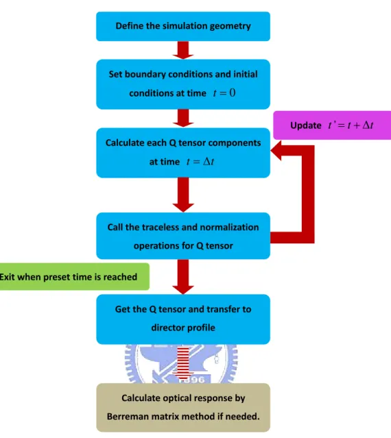
In this section, we combine the Q-tensor approach and the Berrman matrix method to analyze several application examples of LC. Finite element method (FEM) was implemented to solve the partial differential equations of Eq. (2.25) [11]. FEM has the advantages of structure-flexible simulation and less computation time than that with finite difference method. We will focus on the topics that we are interested in. The coupled partial differential equations solver is implemented with COMSOL Multiphysics [12] and is linked to MATLAB. Figure 2-3 shows the flowchart of our simulation procedure.

Set boundary conditions and initial  conditions at time  t=0 

Figure 2-3. The flowchart of the simulation used to calculate the alignment configuration and optical response of nematic LC.

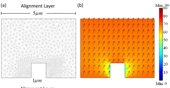
Example 1

In this example, we aim to design a LC cell with each side possessing a square-shaped defect of 1 mμ each side. The structure of the cell is depicted in Figure 2-4 (a). The material parameters of the LC used are given in Table 2-1. The

Calculate each Q tensor components  at time  t= Δt  Call the traceless and normalization  operations for Q tensor  Exit when preset time is reached  Get the Q tensor and transfer to  director profile  Define the simulation geometry  Update  t'= + Δtt   Calculate optical response by  Berreman matrix method if needed.

alignment layers are at the top and bottom of the cell. The cell gap is 4 mμ . The pretilt angle for the alignment layer is70 . We use a mesh that has a higher density near the defect region than that in the rest area. The result is shown in Figure 2-4 (b).

D

As we can see, the LC molecules near the both sides of the defect square can deviate from the alignment direction. The lowest pretilt angle is close to which is almost different from the surface condition. The affected length is around

40D 30D

0.7 mμ started from the square defect. This example illustrates that the smoothness of the substrates used is important for the fabrication of a good LC cell.

Table 2-1: The material parameters of LC used for the simulation.

11 K 11.3pN no 1.506 22 K 7.7pN γ 213 mPaS 33 K 15.8pN ε& 14.1 e n 1.675 ε⊥ 4.0

(a)  Alignment Layer  (b)  5 mμ  

1 mμ   Alignment Layer 

Figure 2-4. The simulation structure with a square of defect. (a) The mesh plot. ( b) The plot of simulation result.

Example 2

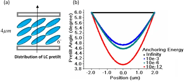
In this example, we discuss the anchoring effect on a LC cell. We set up the LC cell with a pretilt angle of . The schematic showing the distribution of LC pretilt angle from the bottom to the top plate is presented in Figure 2-5 (a). We discuss the LC alignment effect with four different surface anchoring energies: infinity,

6D

3

10− , and (J). The result is shown in Figure 2-5(b). The infinite anchoring energy has an identical pretilt angle of across the thickness of LC cell. The maximum angular deviation across the thickness by using alignment surfaces with an anchoring energy of J can be as large as . This example illustrates that the LC molecules in the center area are not fully aligned with the surface condition when the

6 10− 10−12 10− 6D 12 2.3D