生物系統從序列到結構與功能之計算研究---子計畫三：利用核糖核酸結構預測與核糖核酸-蛋白質互動關係分析推論蛋白質結構(III)

行政院國家科學委員會補助專題研究計畫成果報告

※※※※※※※※※※※※※※※※※※※※※※※※※

※

利用核糖核酸結構預測與核糖核酸-蛋白質互動關係分析推論 ※

※ 蛋白質結構(3/3)

※

※※※※※※※※※※※※※※※※※※※※※※※※※

計畫類別：□個別型計畫 ■整合型計畫

計畫編號：NSC 96－2627－B－009－003－

執行期間：96 年 8 月 1 日至 97 年 7 月 31 日

計畫主持人：胡毓志

共同主持人：

計畫參與人員：劉康平，劉怡馨，陳彥修，許彥超

成果報告類型(依經費核定清單規定繳交)：□精簡報告 ■完整報告

本成果報告包括以下應繳交之附件：

□赴國外出差或研習心得報告一份

□赴大陸地區出差或研習心得報告一份

■出席國際學術會議心得報告及發表之論文各一份

□國際合作研究計畫國外研究報告書一份

執行單位：交通大學 資訊工程系

中 華 民 國

97 年 9 月 15 日

行政院國家科學委員會專題研究計畫成果報告

國科會專題研究計畫成果報告撰寫格式說明

Preparation of NSC Project Reports

計畫編號：NSC 96-2627-B-009 -003-

執行期限：96 年 8 月 1 日至 97 年 7 月 31 日

主持人：胡毓志 交通大學資訊工程系

計畫參與人員：劉康平，劉怡馨，陳彥修，許彥超 交通大學生資所

中文摘要

本計劃首要目標在建立序列－結構－功能間的關係，並深入瞭解RNA/DNA 與蛋白 質分子間交互作用。RNA/DNA、蛋白質及其最後生物功能間的複雜關係與疾病、藥物、 生醫研究密不可分，仍有極大的發展空間，這也是新興的蛋白質體學亟待解決的問題。 本計畫的研究成果，有助於高精確度地分析、預測RNA/DNA 及蛋白質結構與生化網絡 的構成方式。簡言之，即是以序列及結構資訊為基礎，解析蛋白質－RNA/DNA 交互作 用系統。 本計劃包括核醣核酸(RNA)二級結構預測及分類(Chapter 1)、蛋白質－去氧核醣核 酸(DNA)交互作用系統(Chapter 2)，以及蛋白質－核醣核酸交互作用系統(Chapter 3)。三 者間的緊密結合，可以涵蓋由RNA 序列到生物功能間各層次的完整研究。 本計畫所針對的目標有六︰

一、 建立預測RNA 二級結構及 RNA 分類模組。(Chapter 1)

二、 利用 RNA 二級結構及 protein-RNA 嵌合工具預測 protein-RNA 交互作用。 (Chapter 1、3)

三、 將蛋白質功能區域(domain)及蛋白質結晶結構作為定義 protein-DNA 交互作用

的基礎，結合從已知生化路徑中萃取的 protein-DNA 間作用關係，預測未知

生化路徑或擴張已知生化網絡。(Chapter 2)

四、 以已發展完成的protein-ligand 嵌合工具(GEMDOCK)尋找可能的 protein-RNA 交互作用。(Chapter 3) 五、 比較 protein-RNA 與 protein-DNA 交互作用之特性，以建立更完善之預測系 統。(Chapter 1、2、3) 六、 發展protein-RNA 嵌合預測工具及更精確的計分函式，此工具結合物理及生化 知識，可較現有工具更準確地預測 protein-RNA 交互作用及分子表面結合位 置。(Chapter 3) 針對上述提出的六大目標，在本計畫的三年執行期限間(2005-2008 年)，研究團隊成 員共發表論文5 篇，研究成果十分豐碩。整體而言，我們相信在本計畫實行的三年間， 研究團隊已順利達成執行目標，並取得豐富的研究成果。這些成果對於序列－結構－功

Abstract

Our central theme is the study of the sequence-structure-function relationships and protein-RNA and protein-DNA interactions. RNA/DNA molecules are the key players in the biochemistry of the cell, playing many important roles in regulation, catalysis and structural support. These biological interaction networks still are not only hot issues in system biology but also very useful in practical biological research. Hence, it becomes increasingly important for computational biologists to develop reliable and efficient computational approaches to study sequence-structure-function relationships, protein-RNA and protein-DNA interactions, and to predict reliable 3D structures from the sequence level in order to help functional genomics research.

This project covers research areas from RNA, DNA and protein networks of a biological system. Close cooperation between the RNA secondary structure prediction and clustering (Chapter 1), protein-DNA interaction (Chapter 2), and protein-RNA docking system (Chapter 3) will be advantageous and valuable to researchers to find RNA sequence-structure-function relationships and protein-RNA interactions.

The major objectives of this project are listed as follows:

1. Developing a prediction system of RNA secondary structure and clustering. (Chapter 1)

2. Predicting protein-RNA interaction based on RNA structure prediction and protein-RNA docking system. (Chapter 1 and 3)

3. Deriving domain-domain interactions from known protein-DNA complexes and known biochemical pathways to predict protein-DNA interactions and find new biochemical pathways. (Chapter 2)

4. Predicting docking conformation of protein-RNA interaction using GEMDOCK. (Chapter 3)

5. Compare protein-DNA and protein-RNA interaction characteristic to improve prediction quality of protein-DNA and protein-RNA interactions. (Chapter 1, 2 and 3) 6. Developing a new evolutionary protein-RNA docking method and creating a new

protein-RNA binding model by integrating physical-based and knowledge-based scoring functions to reduce calculating quantity and to improve prediction quality of protein-RNA interactions. (Chapter 3)

In summary, we have published 5 papers during 2005-2008. We believe that we have achieved fruitful results in this integrated project. This interdisciplinary research project covers research areas from protein-RNA interactions to protein-DNA interactions. We consider that these achievements will be advantageous and valuable to researchers to study sequence-structure-function relationships and protein-RNA and protein-DNA interactions.

Chapter 1:

Protein/RNA structure prediction and

clustering

1.1 Introduction

RNA plays a crucial role in posttranscriptional regulation. Similar to transcriptional regulation, post-transcriptional regulation is often accomplished by the binding of proteins to specific motifs in mRNA molecules. Most of the current structural bioinformatics research is focused on proteins, and yet thousands of genes produce transcripts exerting their functions without ever producing protein products. A fundamental principle of biology is that a stable 3D structure is essential for biological functions. Many functional RNAs have evolutionarily conserved secondary structures in order to fulfill their roles in a cell. In another word, unlike DNA binding proteins, which recognize motifs composed of conserved sequences, RNA protein binding sites are more conserved in structures than in sequences. Various computational methods for the prediction of RNA secondary structures have been developed. According to the search strategies applied and the structure representations used, they can be roughly classified into the following categories: (1) free energy minimization [1-3] (2) comparative sequence analysis [4, 5] (3) stochastic context-free grammars [6-8] (4) heuristics [9-11] (5) graph theoretical approach [12, 13] and (6) hybrid [14-17]. A lot of works have

been done for single RNA structure prediction; however, as more RNA sequence data have been produced, finding characteristic structure motifs within RNA families becomes very important.

The goal of this section is to understand relationship of RNA/protein structure and function by secondary structure prediction and clustering. We have studied RNA/protein structure prediction and clustering in the past three years, and published four papers as fellow: 1. Y. Hu, “RNA Clustering and Secondary Structure Prediction”, International Conference on Mathematics and Engineering Techniques in Medicine and Biological Science, 2005. 2. S. Ku and Y. Hu, “A Multistrategy Approach to Protein Structural Alphabet Design”,

Biocomp 2006.

3. K. Chen and Y. Hu “Bicluster Analysis of Genome-wide Gene Expression”, IEEE Symposium on Computational Intelligence in Bioinformatics and Computational Biology, 2006

4. C. Huang and Y. Hu “A Two-stage Approach to Finding Common Structure Elements in Unaligned RNA Sequences”, Biocomp 2007

prediction and clustering simultaneously, since some current approaches can now identify common structure motifs from a set of RNAs, they typically assume the given set forms a single family, which is not necessarily correct. The performance of this study is demonstrated on several real RNA families, and showed very promising results.

In the second year (2006), we demonstrated how the structural alphabet can be used with conventional 1D sequence alignment algorithms and presented its results. A comparative study of our alphabet with one of recently developed structural alphabets also showed a competitive result. Moreover, we proposed a new biclustering method based on the framework of market basket analysis in which a bicluster is described as a frequent itemset. As a feasibility test, we compared it with several standard clustering algorithms on a genome-wide yeast microarray dataset, and it showed very promising results.

In the third year (2007), unlike some methods that find consensus structures from a multiple sequence alignment if available or others that align sequences and structures simultaneously, we have developed an approach which separates consensus motif finding from sequence folding. After applying RNA folding algorithms to each sequence of given RNAs as a preprocess, we then combine structure decomposition and Gibbs sampling techniques to identify common structure motifs in unaligned RNA sequences. To demonstrate the performance, we tested it on several RNA families in Rfam. The experimental results show our new approach is competitive with other current prediction systems.

1.2 Motivation

RNA molecules are the key players in the biochemistry of the cell, playing many important roles in regulation, catalysis and structural support. Like proteins, their functions generally depend on their structures. Although structural genomics, the systematic study of all macro-molecular structures in a genome, is currently focused more on proteins, thousands of genes produce transcripts exerting their functions without ever producing protein products. Most of the current structural bioinformatics research is focused on proteins, and yet thousands of genes produce transcripts exerting their functions without ever producing protein products [18-20]. We can easily argue that the comprehensive understanding of the biology of a cell requires, besides proteins, the knowledge of the identities of all functional RNAs (both noncoding and protein-coding) and their molecular structures.

A fundamental principle of biology is that a stable 3D structure is essential for biological functions. Many functional RNAs have evolutionarily conserved structures in order to fulfill their roles in a cell. Some of the functions can be presented by functional motifs, such as several well-understood structurally conserved RNA motifs in viral RNAs, e.g. the TAR and RRE structures in HIV and the IRES regions in Picornaviridae [21]. Although experimental assays for basepairing in RNAs constitute the most reliable method for secondary structure determination, yet it is often difficult and expensive to acquire the 3D spectrum data of RNA molecules [22].

1.3 Methods

We have studied about relationship of Protein/RNA structure and function in the past three years. In the first year, in order to understand RNA structure and function, we have studied how to cluster RNA by its function and predict its secondary structure. This study provides RNA functional classification and RNA structure prediction. The results have been published in International Conference on Mathematics and Engineering Techniques in Medicine and Biological Science. In the second year, in order to understand relationship between RNA and protein structure, we have studied protein structural alphabet design and bicluster analysis of genome-wide gene expression. These studies provide how to analyze/predict protein structure and a new biclustering method based on the framework of market basket analysis in which a bicluster is described as a frequent itemset. In the third year, we have proposed a two-stage approach to finding common structure elements in unaligned RNA sequences, in order to model RNA structure and predict its function more correctly. The detail of these studies are described as fellow:

First Year:

1.3.1 RNA Clustering and Secondary Structure Prediction

Unlike previous studies of RNA secondary structure prediction whose input is either a single RNA sequence or a known class of functionally related sequences, our new method is instead applied to a set of unaligned RNA sequences which consist in an unknown number of classes. In order to find a reasonable partition for a given set of unaligned RNAs without knowing beforehand how many clusters actually existing in this set, we assume that each cluster is likely a functional family that contains characteristic structure motifs. Based on this assumption, our new method is focused on finding significant consensus structure motifs that can be used to characterize the families of RNAs. Since the number of clusters and its size are unknown in advance, we take a generateand-test strategy that iteratively adjusts the hypothesized cluster size until some significant consensus structure elements can be found

associated with this cluster. After a cluster is obtained, all its members are then removed from the given RNAs. We repeat the same separateand-conquer strategy to identify other clusters from the remaining RNAs.

Generate-and-Test

The generate-and-test strategy we use is an adaptive approximation approach that systematically revises the hypothesized cluster size. During the generate-and-test process, the cluster size is defined by a range between an upper bound U and a lower bound L. Without any prior information of clusters, the cluster size is initialized within a range between an upper bound U=n and a lower bound L=0, that is, we first assume that all the given RNA sequences consist in an entire family. To the entire family, a genetic programming-based structure prediction method is applied to look for the fittest consensus structure motifs. If the specificity of the structure motifs associated with a cluster exceeds or equals some pre-specified threshold, the hypothesis of the cluster is accepted, and the cluster along with the associated structure elements will be reported. On the other hand, low specificity suggests that the current hypothesized cluster size is too big to be real and needs to be decreased. In this case, we reduce the current hypothesized cluster, and search the fittest consensus structure motifs and evaluate their specificity again. If the specificity is still lower than the threshold, we further decrease the cluster size. The same process for cluster size reduction can be repeated till we find a cluster with structure motifs of highspecificity. On the contrary, if the specificity is over or equal to the threshold, one of the two possibilities holds: (1) the current cluster is real, and any more sequences added will be harmful to the specificity of consensus structures, or (2) the current cluster found is only a subset of a bigger real cluster. To verify which event actually happens, we increase the cluster size and a new search for the fittest consensus structure motifs is conducted. As each update generates a tighter range for cluster size, we expect the cluster size will eventually converge to the appropriate one.

Secondary Structure Element Prediction by Genetic Programming

The objective here is to learn the structure elements that can be used to distinguish the given functionally related sequences from the random sequences. We modify the fitness function of our previous work [23] on RNA consensus secondary structure prediction to find significant structure elements from a dataset that may contain multiple variable-sized clusters of unaligned sequences.

The fitness function is used to measure the quality of individuals (i.e. candidate structure elements) in a population. The higher the fitness of an individual, the better its chances of survival to the next generation. In the previous work, the input dataset was assumed to be a single class of functionally related RNA sequences. We were interested in those structure

elements that can reflect the characteristics conserved in a family, e.g. the RNA protein binding sites. Derived from the F-score, the fitness function was aimed to balance the importance of two measures, recall (i.e. sensitivity) and precision (i.e. positive predictive value) [10]. It assigns higher values to those structural motifs commonly shared by the given family of RNAs, and rarely contained in random sequences. For a given set of RNA sequences that form a single family only, the fitness function used in [10, 23] can effectively guide the evolutionary process in genetic programming. Nevertheless, when the input dataset contains multiple functional classes, the recall measure may dominate the calculation of F-score if the fitness function treats the entire dataset as a single class. This will mislead the system to find overgeneral elements shared by most sequences. To alleviate the bias, we define a new measure of recall, and present the fitness function as below, where p is the number of positive examples containing motifi, Q is the total number of positive examples, R

is the total number of examples containing motifi, and U is the upper bound of the

hypothesized range for cluster size. ) ( ) ( ) ( ) ( 2 ) ( i i i i

i _{recall motif precision motif}

motif precision motif recall motif Fitness + × × = , (Eq. 1.3.1.1)

where recall(motifi) = p/Q, if p < U or recall(motifi) = 1, if p > U. The value of

precision(motifi) = p/R. By taking cluster size into account, we can better constrain the search

space and allow conserved clusters to emerge more likely instead of being buried in bigger but much less coherent clusters.

Consensus Structure Specificity and Separate-and-Conquer Strategy

The GP (Genetic Programming)-based structure prediction method can find the fittest secondary structure elements according to a given range of the cluster size, while the significance of the cluster found along with its characteristic structure elements highly depends on the range we choose. With proper adjustment of cluster size through the generate-and-test procedure combined with the GP-based prediction method, we can identify a meaningful cluster and the associated characteristic structure elements. The adaptive adjustment of cluster size in the generate-and-test procedure is controlled by the consensus structure specificity. It is defined as the Laplace prior precision. The Laplace prior approach has also been applied to inductive leaning to evaluate the significance of inductive rules [24]. The Laplace prior precision of cluster Ci is given by the formula:

LaplacePriorPrecision(Ci) = (number of positive examples in Ci +1) / (total number of

examples in Ci +2), (Eq. 1.3.1.2)

conserved clusters whose size is too small. For example, the Laplace prior precision of a cluster of 50 positive examples and five negative examples is better than that of a cluster of only five positive examples. Note that the Laplace prior precision is only used to determine the significance of a cluster found, unlike the F-score, which is used to direct the optimization process to find the best structure elements under the constraints of the cluster size. Based on the comparison of the Laplace prior precision with a pre-specified threshold, we adjust the range of cluster size accordingly, and then re-run the GP-based method to predict new structure elements and a new cluster they characterize.

Once a significant cluster is found, we separate all its members out of the given dataset of RNA sequences. We then apply the same procedure to those that still remain in the dataset until the entire set is emptied. This separateand-conquer strategy is effective when no prior knowledge of the identities of the clusters is given. It can automatically partition the given dataset into meaningful clusters, and also identify their characteristic structure elements.

Second Year:

1.3.2. A Multi-strategy Approach to Protein Structural Alphabet Design

The use of frequent local structural motifs embedded in polypeptide backbone has recently shown improvement in protein structure prediction [25-27]. Its success has shed some light on further studies of structural alphabet. We used the proteins classified to all-α fold within the SCOP database (version 1.65) in our study with the aim to build the structural alphabet suitable for all-α proteins. The same approach can be easily applied to other databanks as well.

There are three issues addressed in our study. They are: (1) protein fragment representation, (2) alphabet size determination and (3) structural alphabet definition. Like others, we transform each protein backbone into a series of the dihedral angles (φ and ψ, neglecting ω) [26, 28]. Adapted from [28], the analysis is limited to fragments of five residues since they are adequate for describing a short α helix and a minimal β structure. With the fixed window size of five residues, we slid the window along each all-α protein in SCOP, advancing one position in the sequence for each fragment, and collected a set of overlapped 5-residue fragments. As the relation between two successive carbons, Cαi and

Cαi+1, located at the ith and (i+1)th positions, can be defined by the dihedral angles ψi of Cαi

and φi+1 of Cαi+1, a fragment of L residues can then be defined as a vector of 2(L-1) elements.

Thus, in our study, each protein fragment, associated with α-carbons Cαi-2, Cαi-1, Cαi, Cαi+1

and Cαi+2, is represented by a vector of eight dihedral angles, i.e. [ψi-2, φi-1, ψi-1, φi, ψi, φi+1,

ψi+1, φi+2]. Based on this representation, we totally gathered 1,143,072 fragment vectors.

complex data sets. A self-organizing map usually consists of a regular 2D grid of so-called map units, each of which is described by a reference vector mi = [mi1, mi2, mi3,…, mid], where

d is the input vector dimension, e.g., d = 8, in our case of fragment vectors. The map units are

usually arranged in a rectangular or hexagonal configuration. The number of units affects the generalization capabilities of the SOM, and thus is often specified by the researcher/user. It can vary from a few dozen to several thousands. An SOM is a mapping from the ensemble of input data vectors (Xi=[xi1, xi2, xi3,…, xid] ∈ Rd) to a 2D array of map units. During training,

data points near each other in input space are mapped onto nearby map units to preserve the topology of the input space [29, 30]. The SOM is trained iteratively. In each training step t, distances between a randomly picked input vector xj and all the reference vectors are

computed. The unit with the least distance is then selected as the winner unit and denoted by w. The winner unit and its topological neighbors are updated to move closer to input vector xj

in the input space by the following rule:

m_i(t+1)=m_i(t)+α(t)h_wi(t)|x_j −m_i(t)|, (Eq. 1.3.2.1) where t is time, α(t) is the adaptation coefficient, |xj-mi(t)| is the component-wise

difference between the input vector and the ith reference vector, and hwi(t) is the

neighborhood function acting on the array of units, whose form includes bubble kernel, Gaussian kernel and other more complicated ones. In our study, we used the bubble kernel [29, 31]. Unlike previous works that directly apply SOM to obtain clusters of backbone fragments as the basis to define the structural alphabet, our approach instead uses SOM only for the visualization purpose to predetermine the number of letters in the alphabet.

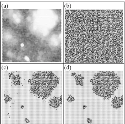
By visual inspection of the trained SOM, we can get a preliminary idea of the number of clusters on the map. The unified distance matrix (U-matrix) is one of the most widely used methods for visualizing the clustering result on the SOM. It shows distances between neighboring reference vectors, and can be efficiently visualized using grey shade [32], as shown in Figure 1.3.2.1(a). In spite of the initial idea of the cluster structure provided by the U-matrix, a systematic method to determine the number of clusters on the map is still desired. We implement a post-process on the Umatrix that is based on the minimum-spanning-tree algorithm. Given the grey levels in the U-matrix, we can build the minimum spanning tree for all the map units, e.g., in Figure 1.3.2.1(b), all map unit are linked in the spanning tree. Based on a threshold of the grey level, we can partition the entire tree into several disconnected subtrees, by removing the links between map units with grey levels below the threshold, as shown in Figure 1.3.2.1(c). Conceptually, it means that we break the links of a distance longer than some threshold. Furthermore, those relatively smaller subtrees left can be also deleted later such that the remaining clusters can maintain a reasonable size, as presented in Figure 1.3.2.1(d). The number of the subtrees finally kept becomes the structural alphabet size. As the SOM can be viewed as a topology preserving mapping from input space onto the 2D grid of map units [30], the number of map units can affect the clustering result. We systematically increase the number of units, and repeat the above process till the alphabet size stabilizes.

Figure 1.3.2.1. Visualization of the trained SOM. (a) the grey shade of the trained SOM,

where darker areas mean larger distances, (b) the minimum spanning tree for the map units, (c)

the disconnected subtrees after removing the links below some threshold and (d) the final

disconnected subtrees after discarding those relatively small ones.

Rather than adapt the two-level approach that first trains the SOM, then performs clustering of the trained SOM [30], after determining the alphabet size, we apply the k-means algorithm to the input data vectors directly to obtain the clusters. The SOM established a local order among the set of reference vectors in such a way that the closeness between two reference vectors in the Rd space is dependent on how close the corresponding map units are in the 2D array. Nevertheless, an inductive bias of this kind may not be appropriate for structural alphabets since the local order does not always faithfully characterize the relation between structural building blocks, and can sometimes be misleading, e.g. forcing the topology to preserve mapping from the input space of α-helix and β-strand to a 2D grid of units could be harmful to clustering. As a result, we use the SOM only for visualization the alphabet size, and rely on the k-mean algorithm to extract the local features from the input data that can actually reflect the characteristics of the clusters respectively. The centroid of each cluster forms the prototypical representation of each alphabet letter. Given the clustering result by the k-means algorithm as the basis of the structural alphabet, we can transform a protein into a series of the alphabet letters by matching each of its fragments against our alphabet prototypes. The control flow of our system named SMK is illustrated in Figure 1.3.2.2.

Backbone Transformation into Dihedral Angles

Protein Fragment Vectors Extraction as Input to SOM, i.e.

[ψi-2, φi-1, ψi-1, φi , ψi, φi+1, ψi+1, φi+2]

Train SOM on Protein Fragment Vectors

Visualizing trained SOM with UMatrix in Grey Levels

Build Minimum Spanning Tree from U-matrix

Partition Minimum Spanning Tree into Disconnected Subtrees

Use number of subtrees as K and Run K-mean Algorithm on Input Vectors

Define Structural Alphabet based on K-means Clusters

Transform Proteins into Structural Alphabet

Figure 1.3.2.2. The system control flow of SMK

1.3.3. Bicluster Analysis of Genome-Wide Gene Expression

As the advent of microarray technologies, numerous datasets generated by massive microarray experiments have drawn a lot of attention to the need for efficient and effective computational methods for gene expression data analysis [33-35]. In general, expression datasets are described by 2-D arrays. One axis represents the genes; the other, the conditions. Each element in the array records the expression level of a gene as a real number, which is usually derived by taking the logarithm of the relative abundance of the mRNA of that gene in a specific condition. Genes with compatible expression patterns are believed to be under identical or related regulatory control. Given appropriate gene clusters, there can be many further applications based on expression behaviors when combined with other biological information such as subcellular localizations, metabolic pathways and intermolecular interactions, and so on [36]. This demonstrates the importance of the finding of expression clusters.

Clustering can be applied to either genes or conditions to obtain expression clusters, i.e., grouping genes according to all conditions, or grouping conditions according to all genes, separately. The most common clustering algorithms include hierarchical clustering [37], self-organizing maps (SOM) [32] and k-means clustering [38], etc. Nevertheless, most of

them only consider global similarity between expression profiles or between condition samples, thereby missing local relationships. They typically assume that functionally related genes behave similarly over all measured conditions, and the conserved condition patterns run across all measured genes. Those clusters found are in a sense aimed to reflect a global pattern of expression data, and yet for most cases in the real cellular processes, expression patterns are common only to a subset of genes under certain experimental conditions [39]. In order to characterize the expression behaviors more accurately, we need a local model instead of a global one. Identifying such local patterns will provide a deeper insight into genetic pathways that cannot be revealed from the point of a global view. As a result, our objective is to develop, beyond the common clustering paradigm, a method capable of discovering in the microarray data local expression patterns in terms of submatrices which we call biclusters. The rows and columns of a submatrix correspond to a subset of genes with similar expression behaviors under a certain subset of conditions, respectively.

Figure 1.3.3.1. A sample of biclusters. A sample gene expression result is represented as a

2D array. In this array, we show two overlapping biclusters that are formed by different subsets of genes and conditions

For example, in Figure 1.3.3.1 we show a sample gene expression result represented by a 2D array, where the rows stand for different genes; the columns, various conditions. In this array, there are two submatrices each of which consists of different subsets of genes and conditions.

Several methods from various research fields have been proposed to perform clustering which take into account rows and columns at the same time. Though named differently, such as biclustering, local clustering, coclustering, direct clustering, bidimensional clustering, or block clustering, etc. [40-42], they all refer to the same class of algorithms which identify subsets of rows and subsets of columns by performing simultaneous clustering of these two dimensions. These methods can be further categorized according to the types of biclusters they intend to identify. The categories of biclusters may vary from the simplest one which contains only constant gene expression levels, or those with constant values in the rows or the columns, to more complicated ones which contain coherent expression levels with low variance, or others that only maintain a coherent expression trend without considering

specific expression values [43]. It is inevitable that there exists a tradeoff between the complexity of search strategy and the expressiveness of the biclusters identified. The type of biclusters to find determines the complexity of search strategies applied by the biclustering algorithms. The approaches previously proposed include greedy iterative search [40], divide-and-conquer [41], exhaustive enumeration [44] and probabilistic modeling [45], etc. In this study, we propose a new approach called PIFP (Progressive Iterative Frequent Pattern) to biclustering based on frequent itemset identification [46], which is not aimed at resolving all the issues in the biclustering problem, but instead at demonstrating the feasibility of tackling the problem from a different perspective. To fairly compare biclustering methods is not easy as each approach may formulate the same problem differently, and consequently applies different algorithms. Due to the inherent bias, their performance may vary in different scenarios. Recently, a systematic comparison methodology for biclustering has been proposed, which defines the common settings for most of the biclustering approaches [47]. Based on this testing methodology, we conducted the validation using prior knowledge, i.e. gene ontology. Several conventional clustering methods and some current biclustering systems were also tested for comparison in our studies. The conventional ones are hierarchical clustering [37], k-means [38], self-organizing maps (SOM) [32] and principle component analysis (PCA) [48]; the biclustering algorithms include OPSM [39], ISA [49], CC [40], xMotifs [50], BiMax [47] and SAMBA [49]. We demonstrate that our new approach outperformed these systems in the experiments.

Unlike previous approaches, we transform the biclustering problem into a frequent itemset finding task, which is a welldefined activity in market basket analysis. To illustrate the idea, let us first consider a market basket containing a collection of items purchased by a customer in a single transaction. Retailers usually accumulate huge collections of transactions over time, and one common analysis run against a transaction database is to find sets of items (or itemsets) that appear together in many transactions. We call an itemset a frequent itemset if the percentage of the transactions that contain this itemset, which is called support, is above a userspecified threshold. As the items in a frequent itemset co-occur in many transactions, some association is expected among them. Motivated by this observation, we characterize a bicluster containing related genes and relevant conditions by a frequent itemset where genes or conditions are treated as items, and the conserved expression behaviors correspond to the associations.

In microarray experiments, there are different sources of systematic errors [51]. Normalization refers to the attempts to remove such error that affect the measured expression levels. Although normalization alone cannot control all the systematic variations, it is still crucial to subsequent expression data analyses as the expression data may vary significantly from different normalization processes. We tested several normalization methods, including geometric mean normalization, rank normalization, quintile normalization and Spellman et

al.’s Z-score [52, 53]. As some pilot tests favored the Z-score approach, we decided to adopt the normalization procedure of Spellman et al., who normalized the expression level of each gene so that the mean and the deviation for each row and column are zero and one respectively. In addition to normalization, discretization is another preprocess required of PIFP as a bicluster is described by a frequent itemset. We partitioned numeric gene expression values into a set of intervals; as a result, the original expression data matrix can be viewed as a database of transactions. Several discretization procedures were tried to define intervals [54, 55]. The intervals may be determined by some specific thresholds, such as the median, the top N% expression value, or even pre-specified ad hoc values. On the other hand, we can partition expression levels into J intervals of equal size, e.g. J=10. It is usually difficult to define appropriate thresholds beforehand, and our pilot tests showed that the equal-interval partition method worked reasonably well, thus in the following experiments we adopted this discretization procedure with J set to 10.

Figure 1.3.3.2. The PIFP system flow, in which we added the filtering and masking

procedures to rule out spurious biclusters and the ones already found. These procedures have proved effective in producing more biclusters than the original FP-growth method.

There have been many various approaches to frequent itemset finding, and one of the widely used methods is FPgrowth [46]. Unlike its relevant pioneer approaches, e.g. Apriori [55, 56], FP-growth only needs to scan the database twice without the time-consuming candidate-generation process. The first scan of a database derives an ordered list of frequent itemsets above some pre-specified support threshold. For the second scan, FP-growth performs a database projection of the frequent itemsets in the order that they are in the ordered list, and constructs a compact data structure called FP-tree, which stores the complete

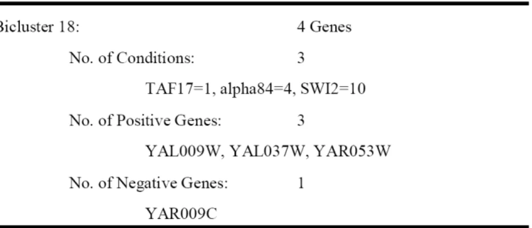
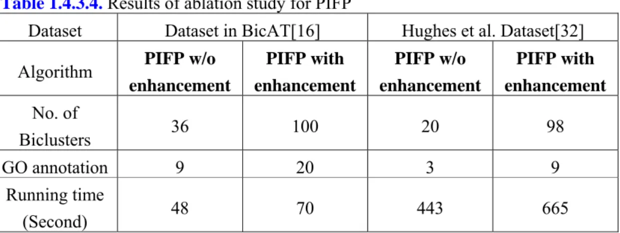
frequent itemset information. This significant reduction on the number of necessary database scans dramatically increases its efficiency. We developed PIFP based on FP-growth. It extends FPgrowth in two directions. First, we embed a filter in PIFP to rule out those spurious itemsets by removing any itemset of less support if it overlaps with others over 75%. Second, we add a feedback loop to PIFP in order to identify weaker (i.e. with less support) frequent itemsets which may have been clouded by other stronger frequent itemsets. By masking out from the expression matrix the itemsets already found, PIFP is able to progressively identify more frequent itemsets than conventional FP-growth approaches. Our ablation experiment in the following section proves the effectiveness of these extensions. Given only two parameter values, minimum support s and minimum itemset size i, PIFP is capable of identifying overlapped biclusters presented as frequent itemsets. The system flow of PIFP is presented in Figure 1.3.3.2. A sample output of a bicluster is shown in Fig. 1.3.3.3. It contains information such as the total number of genes in this bicluster, who they are (e.g. gene or ORF names), the positive-correlated genes, the negative-correlated genes, and the corresponding conditions, etc.

Figure 1.3.3.3. A sample output of PIFP. It shows there are 4 genes in bicluster18, and three

conditions involved. Three of the genes are positive-correlated, and only one is negative-correlated.

Third Year:

1.3.4. A Two-stage Approach to Finding Common Structure Elements in

Unaligned RNA Sequences

Given functionally related RNA sequences, there are currently three main approaches to the finding of common secondary structures [57]. The first approach aligns sequences using standard multiple sequence alignment tools, e.g. ClustalW [58], and then detects consensus

secondary structures based on mutual information, free energy or sequence covariance [4, 59, 60] etc. However this approach strongly depends on a reliable multiple sequence alignment. It is not suitable for RNAs with low sequence similarity. An alternative approach is to fold sequences and align structures at the same time. Though this approach can be applied in the case of unavailability of multiple sequence alignment, its high computational complexity restricts its practical use [61-63]. If there is no enough sequence conservation, and the complexity of structure motifs exceeds the pragmatic limit of the above approaches, we may take the last approach. It first predicts the secondary structure for each sequence, and then aligns the structures directly [16, 64, 65].

There are several important features in our method. First, it is applicable to unaligned RNA sequences with long flanking regions and low sequence similarity. Second, it has flexibility in incorporating new tools for single RNA global structure prediction in the first stage. Third, secondary structures predicted in the first stage are transformed to an abstract form that helps constrain the search space of consensus motifs.

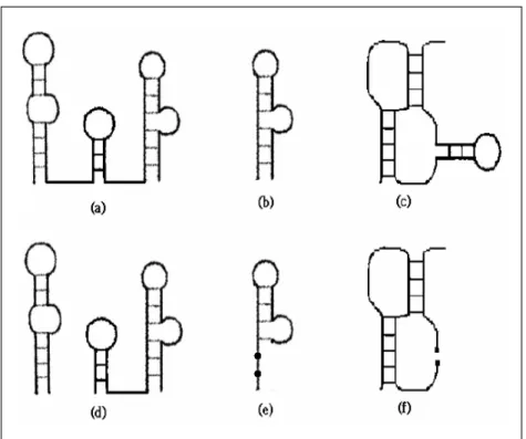
Figure 1.3.4.1. Positive and negative examples of structure motifs. (a)(b)(c) are legal

structure motifs. Each satisfies all three conditions of a legal structure motif. (d)(e)(f) are the

negative examples relative to (a)(b)(c) respectively, where (d)(f) are not continuous structures,

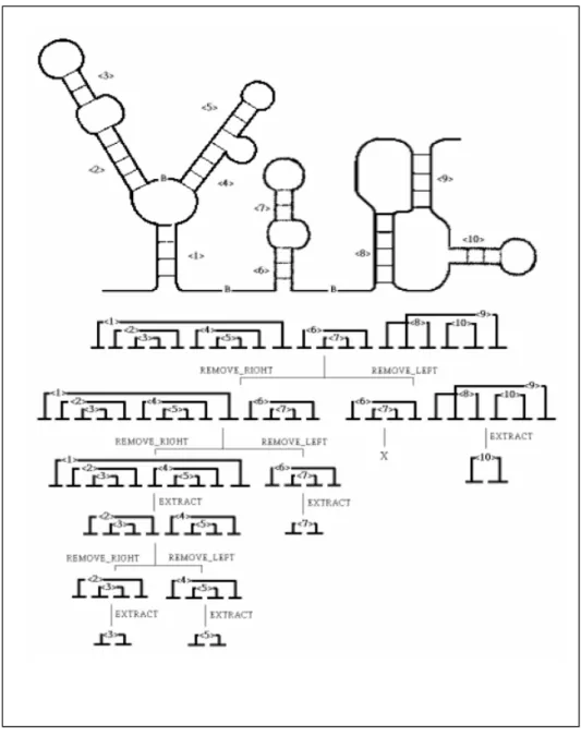
Figure 1.3.4.2. An example of structure decomposition. The given structure (stem <1> to

<10>) is not a component motif as it has several bifurcation sites, marked by “B”. We first remove its rightmost and leftmost component respectively to produce two legal substructures, one composed of stem <1> to <7>; the other, <6> to <10>. We later generate two substructures from stem <1> to <7>. They are stem <1> to <5> and stem <6> to <7>. These two structures are component motifs since they have no bifurcation site, and smaller legal substructures can be extracted from within, e.g., stem <2> to <5> extracted from structure <1> to <5>. We keep decomposing a structure until we reach its basic singlestem component, e.g. <3>, <5> and <7>. On the other branch, stem <6> and <7> are found to already occur in the left branch, therefore, they are considered redundant and will not be further processed. Stem <8> to <10> is also a component motif which is a pseudoknot containing stem <10>, the last legal substructure extracted.

Our proposed method adopts the last approach, but the objective of our system is to find consensus structure motifs within a set of RNAs rather than a multiple global structure alignment. We define a legal structure motif for an RNA family as a commonly shared

structure: (1) that is folded from continuous nucleotides, (2) that begins with a 5’segment of a stem, and ends with a 3’segment which may be the half of another stem or paired with the first 5’segment, and (3) that has no unpaired 5’or 3’segment between the first 5’segment and the last 3’segment. Some positive and negative examples are shown in Figure 1.3.4.1. For each predicted structure from a folding algorithm, we exhaustively decompose it and enumerate all the possible substructures that comply with the three constraints above. A legal structure motif can be further defined as a component motif if it satisfies all three constraints above, and cannot be broken into smaller legal structure motifs, e.g. Figure 1.3.4.1(b) and (c). For a structure with only one component, we can discard either the outermost paired segments or pseudoknots to extract a smaller legal substructure by EXTRACT. On the other hand, given a structure with more than one component, we can divide it into two legal substructures by removing the leftmost (i.e. REMOVE_LEFT) or the rightmost component (i.e. REMOVE_RIGHT). One example of structure decomposition is illustrated in Figure 1.3.4.2. By applying EXTRACT and REMOVE recursively when applicable, we can decompose any given structure and enumerate all its possible legal substructures that will be later transformed into the search space of consensus motifs.

The occurrences of a consensus motif in a family are rarely the same in every detail of their structures. For example, the size of stems or loops may vary among motif occurrences in different family members, and some may even contain extra bulges or internal loops, e.g. X83878.1/168-267 and Z99107.2/86084-86183 of Purine riboswitches in Rfam with their secondary structure motifs shown in Figure 1.3.4.3 (a). According to the alignment, the first stem of Z99107.2/86084-86183 has a symmetric bulge (small internal loop) consisting of CUCA, which does not exist in X83878.1/168-267. Besides, X83878.1/168-267 has a smaller symmetric bulge in the second stem and a shorter third stem when compared with Z99107.2/86084-86183, while it has longer first and second stems. To accommodate these minor differences between motif patterns (i.e. motif occurrences) in a family, we represent the decomposed substructures by an abstract shape [64], which corresponds to the common secondary structure, as illustrated in Figure 1.3.4.3 (b). By abstraction, these abstract shapes form a much smaller search space where we can find consensus motifs more efficiently.

Figure 1.3.4.3. Motif structure patterns in two members of the Purine riboswitch family in

Rfam and the abstract shape for the motifs. (a) Consensus secondary structure between X83878.1/168-267 and Z99107.2/86084-86183 of Purine riboswitches in Rfam. (b) Ignoring the minor differences (e.g. different sizes of stems, loops or bulges) and focusing on the common relationship among the stems, we can represent the consensus structures by one abstract shape.

Gibbs sampling is one of the MCMC (Markov Chain Monte Carlo) algorithms. In Gibbs sampling, we iteratively sample each variable conditioned on the most recent values of the other variables. Starting with a set of initial values of all the variables, we cycle through the sampling process for each single variable in any order until the values of all the variables converge to a stable state. Under this framework, the given RNAs are the variables, and the motif patterns are treated as their values. Our goal here is, by Gibbs sampling, to find the appropriate value (i.e. motif pattern) for each variable (i.e. RNA) such that the values can reach a stable distribution which corresponds to a consensus structure motif.

We define the similarity between two structure patterns, si and sj, as the following:

otherwise sim(si , sj) = w1*seqalign(si , sj)+w2*structalign(si , sj). (Eq. 1.3.4.2)

RLD(si , sj) = | len(si) – len(sj) | / max( len(si) , len(sj) ). (Eq. 1.3.4.3)

where RLD(si , sj) is the relative length difference between si and sj, len(sk) is the sequence length of structure sk. The seqalign(si , sj) is the sequence alignment score based on the Needleman-Wunsch algorithm [66], assuming match=1, mismatch=0 and gap=-1, and structalign(si,sj) is the structure alignment score computed by RSmatch [67]. Both seqalign(si,sj) and structalign(si,sj) are normalized between zero and one. Note that we assign zero to sim(si,sj) directly when RLD(si,sj) is greater thanθL to save the time for the computation-intensive alignment procedures. The motivation behind this is our observation of most families in Rfam shows that the relative length difference between family members is usually insignificant, which makes it an effective filter. In eq.(1.3.4.2), sim(si,sj) is computed as the weighted sum of the sequence and structure alignment scores, where w1+w2=1.

The Gibbs sampling process in our system starts with an initial state of a consensus motif represented by a set of seeds, SEED, each of which is a possible occurrence of the motif in a particular RNA sequence. In each iteration, we sample the motif patterns for one RNA, e.g. R, conditioned on the currently selected motif occurrences in the others, and a structure pattern pi∈R will be chosen as a new seed (i.e. a new motif occurrence) if it satisfies either of the following conditions.

If R does not currently have a seed in SEED, then

∑

∈ ⋅ = SEED s j k p i k j SEED sim p s

p argmax 1/| | ( , ) (Eq. 1.3.4.4) under the constraint that

s SEED s k i k s p sim SEED ⋅

∑

>θ ∈ ) , ( | | / 1

If R already has a seed in SEED, then

∑

∉ ∈ ⋅ − = R s SEED s j k p i k k j SEED sim p s p , ) , ( ) 1 | /(| 1 max arg (Eq. 1.3.4.5)

under the constraint that

s R s SEED s k i k k s p sim SEED − ⋅

∑

>θ ∉ ∈ , ) , ( ) 1 | /(| 1

As we iterate over every RNA, we can either add new patterns as new motif occurrences when the above condition is satisfied, or delete old seeds from the seed set if they no longer meet the constraint. We update the set SEED with the aim to increase the total pairwise pattern similarity simtotal(SEED) defined below. We repeat the same sampling process until no

change of motif occurrences can be made to improve simtotal(SEED).

sim SEED sim s s s_i s_j SEED

j i j i total =

∑

∀ ∈ ≠ , , ) , ( ) ( , (Eq. 1.3.4.6)

The initial seeds determine where and how fast Gibbs sampling converges, and the size of the initial seed set does not need to be equal to the total number of the RNAs given. Since we can start Gibbs sampling with different initial seeds, it can terminate at various sets of final seeds. When Gibbs sampling stops after it converges, the size of converged SEED will ideally be equal or approximate to that of the given RNA family, and the seeds per se are the predicted occurrences of a consensus motif. According to simtotal, we rank all the motifs to

which Gibbs sampling converges, and report them in a sorted list after the user specifies the number of top-ranked motifs required in the output.

1.4 Result

First Year:

1.4.1. RNA Clustering and Secondary Structure Prediction

Two types of quality were considered to evaluate the performance of our method. One is to measure the agreement between the predicted clusters and the actual cluster identities; the other, to quantify the agreement between the predicted structure elements and the actual structure assignment. Since no other current approaches known to perform clustering and structure prediction in parallel, no comparative study can be done. Instead we applied the widely-used precision and recall to measure the first quality; the Matthews correlation coefficient [68], to measure the second quality.

For each sequence in the data set, two secondary structure assignments were compared by counting the number of true positives Pt (base pairs exist in actual assignment and are

predicted), Nt true negatives (base pairs do not exist in actual assignment and are not

predicted), false positives Pf (base pairs do not exist in actual assignment but are predicted)

and Nf false negatives (base pairs exist in actual assignment but are not predicted),

respectively. The Matthews correlation coefficient can then be computed as: ) )( )( )( ( _{t f t f t f t f} f f t t P P N P P N N N N P N P C + + + + − = (Eq. 1.4.1.1)

Given that the sequence length is sufficiently large, the Matthews correlation coefficient can be approximated in the following way [69].

f t t f t t P P P N P P C + ⋅ + ≈ (Eq. 1.4.1.1)

With the published/curated alignments, we can calculate the Matthews correlation coefficient. Higher correlation coefficients mean more accurate structure predictions.

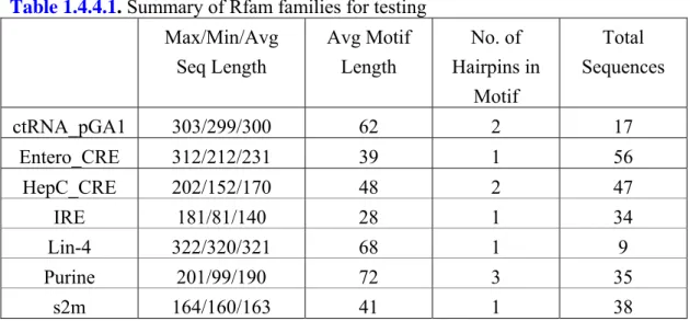
Table 1.4.1.1. Summary of the RNA families used in experiments. The first row shows the

total number of sequences in each data set. Row 2 to 4 present the minimum, the maximum and the average sequence length respectively. The fifth row gives the standard deviation of sequence length.

Dataset 16s RNA IRE-like Viral 3’UTR

Total Sequences 34 56 18

Min Seq Length 90 117 37

Max Seq Length 108 330 137

Avg Seq Length 97.59 202.93 63.89 Seq Length Std 3.77 59.31 25.95

Our algorithm is designed to automatically partition a given set of unaligned RNA sequences into meaningful clusters, each with characteristic conserved secondary structure elements. The number of real clusters and the distribution of cluster size may affect the prediction of partitions and characteristic structure elements. To measure their effect on the performance, we tested our method on different datasets with various RNA families. We used three families, including 16S RNA, IRE (Iron Response Element) and viral 3’UTR as summarized in Table 1.4.1.1, to prepare the test datasets. They have been used in previous experiments and published in literature [10, 69]. The sequence data and the correct structure elements can be accessed at public databases [70, 71]. The 16S RNA dataset contains 34 archaea 16S ribosomal sequences originally derived from a set of 311 sequences extracted from the SSU rRNA database. The archaea set of 311 sequences was further reduced to 34, filtering out the sequences that miss base assignments or are greater than 90% identical. The IRE dataset was constructed by Gorodkin et al.[69] from 14 sequences from the UTR database. They modified the IREs and their UTRs to make the search more difficult. By iteratively shuffling the sequences and randomly adding one nucleotide to the IRE conserved region, they built a set of 56 IRE-like sequences from the 14 IRE UTRs. The third data set includes 18 viral 3’UTRs each of which contains a pseudoknot. Seven of the RNA sequences are the soil-borne rye mosaic viruses; the others are the soil-borne wheat mosaic viruses.

Table 1.4.1.2. Summary of the experimental results. Table (a), (b) and (c) present the result for the dataset containing IRE and viral 3’UTR, 16S RNA and viral 3’UTR, IRE and 16S RNA, respectively.

(a)

IRE+viral 3’UTR Recall Precision Matthews

IRE 0.97 0.99 0.97

Viral 3’UTR 0.71 0.95 0.79

(b)

16s RNA+viral 3’UTR Recall Precision Matthews

16s RNA 0.97 0.95 0.83

Viral 3’UTR 0.77 0.98 0.77

(c)

IRE+16s RNA Recall Precision Matthews

IRE 0.73 0.99 0.85

16s RNA 0.81 0.73 0.67

On the basis of the three real families of RNA sequences, we tested our method on each possible pair of the families, i.e. 16S RNA/IRE, 16S RNA/viral 3’UTR, and IRE/viral 3’UTR. In each run of the experiment, no information regarding the number of families or the family size was given to the algorithm beforehand. One purpose of this experiment is to analyze the effect incurred by the distribution of cluster size in a dataset. Furthermore, as the real conserved structure elements differ in various families, we can also observe how the interleaving of distinct structure motifs within a single dataset may affect the prediction process. The results are presented in Table 1.4.1.2, and some partial predicted secondary structures are shown in Figure 1.4.1.1.

Figure 1.4.1.1. A partial result of the predicted RNA motifs. The numbers above the

sequences are the indices of the nucleotides. The predicted and the published motifs are both shown for reference.

Second Year:

1.4.2. A Multi-strategy Approach to Protein Structural Alphabet Design

We tested our approach on the all-α proteins in SCOP. By this experiment, we show that our method can produce an appropriate structural alphabet for describing these all-α proteins. After transforming protein backbones into dihedral angles and extracting protein fragments, we trained the SOM on these dihedral angle vectors.

Three issues were addressed in the experiments. First, the meaningfulness of the structural alphabet size in terms of the number of clusters was presented by showing the size stability given various parameters. Second, we demonstrated cluster cohesiveness by visual superimpositions of protein fragments as well as computed the intra-cluster and inter-cluster distance. Third, we proved the fragment clusters found were not arbitrary by comparing our result with that from a random background.

Figure 1.4.2.1. The variance in the number of clusters produced by the SOMs of varying

sizes. There exists a distinctive plateau that suggests the cluster number has stabilized.

Since the number of map units has influence over the SOM’s clustering behavior, to obtain the optimal number of clusters, we varied the number of units on the map until the number of clusters found became steady. The results are shown in Figure 1.4.2.1, which indicates a distinctive plateau within the range between nine and twelve. Because eleven is the most frequent number of clusters on the plateau, as shown in Figure 1.4.2.2, it is designated as the structural alphabet size.

Figure 1.4.2.2. The frequencies of cluster numbers. It shows 11 is the most frequent

number of clusters.

To further confirm the general geometric regularities characterized by the structural alphabet, we also built a negative all-α protein fragment set for comparison. The negative set was derived from the real all-α protein fragment vectors prepared earlier by rotating the dihedral angles at random (increase or decrease) within a certain degree, e.g. 30° in our analysis. We compared the clusters produced by clustering on the real vector set and on the negative control set. Insignificant difference suggests that the alphabet we found could be arbitrary. Our experiments (see Figure 1.4.2.3) show that clustering on the negative control

set cannot even produce consistent clusters, which supports our hypothesis that the clusters found from the real fragment vectors reflect the classes of local protein structures; otherwise, these clustering results would have been similar.

Figure 1.4.2.3. The variance in the number of clusters produced by the SOMs of varying

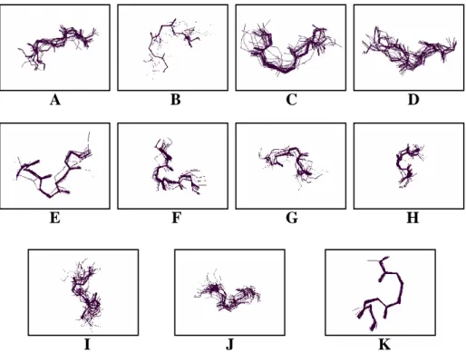
sizes trained on a negative fragment set. It shows no sign of convergent cluster number. Given the size, we ran the k-means algorithm on the input fragment vectors to find the twelve clusters by which to define the structural alphabet. Figure 1.4.2.4(a) and (b) shows the fragment superimpositions for the alphabet. Even though the fragment structures do not superimpose perfectly, yet the general structural cohesiveness of each category is quite evident. In addition, we computed the Euclidean distances from each fragment in a given cluster to its centroid. The average of these within-cluster distances was then compared with the center-to-center distances between clusters as presented in Table 1.4.2.1. It shows that in most cases, the center-to-center distance between any two clusters is greater than the mean distance of all vectors in that cluster from its center plus one standard deviation. The result indicates that the individual clusters are fairly well separated from each other.

A B J I E F G H D C K

Figure 1.4.2.4(a). The superimposition in wireframe format for the structures of each structural cluster found by SMK.

A B J I E F G H D C K

Figure 1.4.2.4(b). The superimposition of the structures of each structural cluster found by

Table 1.4.2.1. Summary of within-cluster distances and center-to-center distances.

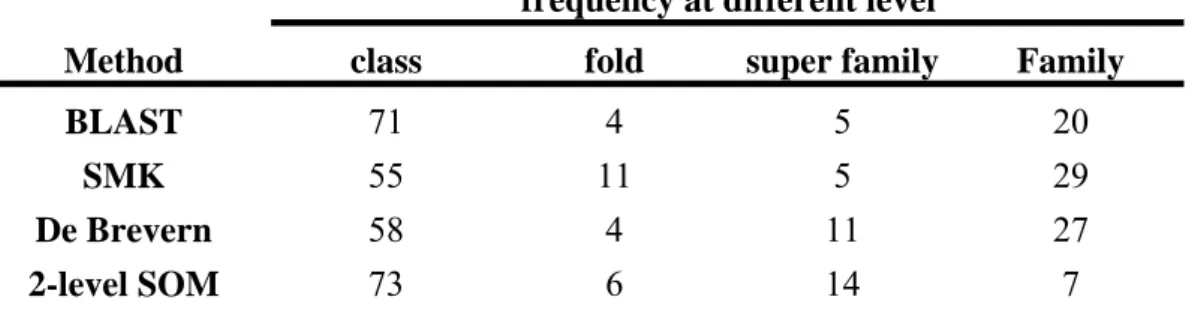
The detection and analysis of structural similarities between proteins allows deeper insight into their functional mechanisms and relationships. To search for structural similarities, the structural alphabet provides a good basis on which to work with a 1D representation. As a result, numerous 1D alignment algorithms can be used, with minor modifications, to detect structural similarities. In our experiments, we first transformed the 3D structures of proteins into a 1D sequence of the letters in our structural alphabet. To demonstrate the applicability of the alphabet, we used FASTA to search for structural similarities between a query protein and a bank of proteins, using an identify matrix of our alphabet letters to find maximal exact matches. For comparison, we also conducted the same tests also using FASTA but based on different structural alphabets, one developed by de Brevern et al. [72], the other by the two-level SOM approach [30]. As the baseline reference, we used BLAST with the standard 20 amino acid letters to find the best sequence hit.

Table 1.4.2.2. Summary of frequencies at the lowest common level. The first column

shows the methods used in the experiments. The remaining columns present the frequency for different levels at which the query and the best hit are both located.

frequency at different level

Method class fold super family Family

BLAST 71 4 5 20

SMK 55 11 5 29

De Brevern 58 4 11 27

Table 1.4.2.3. Summary of average RMSD and standard deviation between the queries and

the best hits.

Method mean (RMSD) sd (RMSD) BLAST 8.953744 4.764597 SMK 7.290972 3.934283 De Brevern 8.076746 4.819178 2-level SOM 10.38624 5.217078

The proteins used in the experiments were selected from the all-α proteins in SCOP. After filtering out those with more than 30% sequence similarity, we have totally 1055 proteins. For each run of the experiment, we randomly picked one protein as the query, and then matched it against the rest, using FASTA or BLAST with different alphabets. Given the best hit, we computed the RMSD between the query and the hit, and recorded the lowest level in the SCOP hierarchy at which the query and the hit are both located, i.e. class, fold, superfamily or family. Smaller RMSD and lower common level in SCOP hierarchy indicates higher structural similarity. We repeated the same experiment for 100 times and the results are summarized in Table 1.4.2.2 and Table 1.4.2.3. According to Table 1.4.2.2, we notice that our method SMK and de Brevern et al.’s both produced higher frequencies at lower common levels than the other two methods. This suggests that our structural alphabet and de Brevern et

al.’s can better characterize the SCOP hierarchy. Table 1.4.2.3 shows that SMK has the lowest mean RMSD and standard deviation among all.

In this study, we propose a multi-strategy approach to designing the structural alphabet which allows local approximation of protein 3D structures as well as enables the applications of 1D alignment algorithms to search for 3D structural similarities. The success of the alphabet design depends on three crucial factors. First, it is the protein fragment representation, which determines what and how 3D structural characteristics to be approximated, e.g. thermodynamic stability, amino acid physicochemical properties, amino acid usage in known proteins, distances, dihedral angles, bond lengths, bond angles, etc. The effects of the representation selected are entangled with the performance of the learning approach we apply to develop the structural alphabet. Overcomplicated representations can sometimes lead to overfitting. To avoid this problem, we currently focus on the dihedral angles. Other features can be easily included in the representation if proved necessary.

The second factor is the size of the alphabet. We took advantage of the SOM as a visualization tool that helps determine the alphabet size. By systematically varying the number of map units on the map, we visualized the clustering behavior of the SOM. Our experiments showed a distinct plateau corresponding to the convergent number of clusters,

compared with the increasing number of clusters in the results of clustering on the random negative control dataset. This suggests that the structural alphabet size we found is not arbitrary.

Various types of algorithms have been applied to clustering local protein 3D fragments into a limited set of fold patters, e.g. self-organizing maps (SOM), hidden Markov models (HMM), neural networks, hierarchical clustering, k-means clustering, etc. Each has its own learning bias and inherent limitations. For example, the topology (e.g. number of layers or map units) of neural networks, the SOM and the HMM strongly affect the performance. The value of k in kmeans algorithm determines the clusters. As a consequence, the third factor is the learning algorithm. In our study, we took a multi-strategy approach. We first used the SOM and the minimum-spanning tree algorithm to determine the alphabet size, and then applied the k-means algorithm to group fragments into meaningful clusters. The number of map units in the SOM and the value of k in k-means are not prespecified in advance, but instead determined systematically. To verify the correspondence of our structural alphabet letter to the fold patterns, we computed the average within-cluster distance for each alphabet cluster as well as the distance across clusters. The small average within-cluster distance and the relatively large between-cluster distance demonstrate the significance of the structural alphabet we found. Furthermore, the visualized superimposition of protein fragments in each cluster also justifies the structural cohesiveness.

The objective of the study is to propose a new approach to developing the structural alphabet. To verify its usefulness, we tested it on the all-α proteins in SCOP, and the experimental results show its promising applicability. After the success on the all-α proteins in SCOP, we plan to test our method on different data banks to further verify its feasibility and generality. Also as mentioned above, the representation is a crucial factor in the alphabet design. We will consider other structural features besides dihedral angles, add more useful features to enhance our structural alphabet, and test the new approach on other families in SCOP.

1.4.3. Bicluster Analysis of Genome-Wide Gene Expression

There are two objectives in our experiments. One is to demonstrate the superiority of PIFP to those standard clustering methods in terms of identifying more meaningful gene groups related to GO categories. The other is to show PIFP’s competitive performance compared with other current biclustering algorithms.

clustering algorithms. One dataset contains 6335 genes with 121 conditions which were obtained by combining expression profiles from several gene expression experiments [37, 53, 73-78]. This dataset was used in our pilot tests to select the appropriate normalization and discretization procedures for PIFP. We tried different normalization and discretization methods as mentioned earlier, and settled on the one with the best performance. The second dataset is the one used by Hughes et al. [79], which contains 6325 genes and 300 conditions. We tested PIFP on this dataset and compared with several representative conventional clustering algorithms. In order to keep the consistency, instead of reimplementing these algorithms or using any ad hoc versions, we adopted in our experiments Cluster3.0 [37], which provides hierarchical clustering, k-means, SOM and PCA, and also has been used in other published similar experiments [49]. In addition, we also included the fuzzy c-means method in our experiments [80].

The quality measure for a cluster is the p-value based on the widely used hypergeometric distribution [80, 81], defined as below,

⎟⎟ ⎠ ⎞ ⎜⎜ ⎝ ⎛ ⎟⎟ ⎠ ⎞ ⎜⎜ ⎝ ⎛ − − ⎟⎟ ⎠ ⎞ ⎜⎜ ⎝ ⎛ =

∑

= N M x N K M x K p K N z x ) , min( , (Eq. 1.4.3.1)

where M is the total number of genes, N is the size of the cluster, K is the total number of genes annotated in some GO [82] category, and z is the number of genes within this cluster in common with this GO category. This measure takes into account both the cluster size and the number of clusters found with respect to the correlation with GO categories. The smaller the p-value, the more consistent the cluster with the annotations. We took the negative logarithm of the p-value to increase the readability.

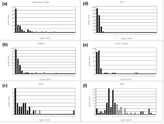
Following [37] to use the default parameter settings in experiments, with Cluster3.0, we tested hierarchical clustering, k-means, SOM and PCA on Hughes expression data. We plot the –log(p-value) vs. cluster count distribution for each of the above methods, as shown in Figure 1.4.3.1(a) to Figure 1.4.3.1(d) respectively, and the results of fuzzy c-means and PIFP are presented in Figure 1.4.3.1(e) and Figure 1.4.3.1(f). In each histogram, we show the cluster count distribution for –log(p-value), and each bar represents the number of clusters with the corresponding –log(p-value) ranging from 1 to 30.

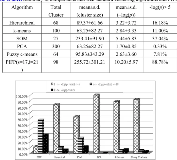
We also summarize the total number of clusters found, the mean and standard deviation of cluster size and –log(p-value) as well as the proportion of clusters with –log(p-value)>5 in Table 1.4.3.1. It is interesting to see that the standard deviation of cluster size is quite large. This seems to agree with the real world that various gene groups of different size perform

very different biological functions. We further divide the values of –log(p-value) into three intervals, and show their proportion distributions for all algorithms in Figure 1.4.3.1. It indicates that the quality, measured by –log(p-value), of the clusters found by the standard clustering algorithms mostly falls within the first interval (i.e. 1≤–log(p-value)≤5), but on the contrary, most of the biclusters identified by PIFP cover the other two. All the evidence provided by Figure 1.4.3.1, Figure 1.4.3.2 and Table 1.4.3.1 clearly shows that PIFP outperforms all the standard clustering algorithms in our experiments.

(a) (b) (c) (d) (e) (f)

Figure 1.4.3.1. The cluster count distribution of –log(p-value) for each algorithm: (a)

hierarchical clustering, (b) k-means, (c) SOM, (d) PCA, (e) fuzzy c-means and (f) PIFP. We partition the value of –log(p-value) into three intervals and present the distribution with bars of different styles to increase readability. Also note that the clusters with –log(p-value)>30 are included as 30 in order to save figure space.