The Applications of Least-Square Sphere Fitting in Digital Camera

(1)

THE APPLICATIONS OF LEAST-SQUARE SPHERE FITTING IN DIGITAL CAMERA

Shih-Ming Chen (

陳世明

) and Chiou-Shann Fuh (

傅楸善

)

Department of Computer Science and Information Engineering

National Taiwan University

Taipei, Taiwan, R.O. C.

Tel: 886-2-23625336 ext. 327

e-mail:

p90013@csie.ntu.edu.tw

ABSTRACT

In general image processing such as binary threshold, brightness, contrast stretch, histogram equalization, and so on are pixel operation. The result always can converge to a pixel re-mapping operation. The disadvantage of traditional method does not consider the background or the environment non-uniformity problem. Therefore it is hard to decide a perfect threshold without a uniform background or the image does not look natural after histogram equalization. In this paper, we will detect the luminance variation vector and then normalize to uniform luminance with a uniform scene assumption, and in image post-processing we assume the image is natural, therefore the pixel re-mapping table is continuous.

1. INTRODUCTION

Background normalization problem always prevent from applying image processing directly. Figure 1 shows an image with non-uniform brightness on the surface. If we directly apply binary threshold operator on Figure 1, the result is shown in Figure 2. We can find some of rice in the corner will disappear because the non-uniform brightness will cause the dark corner. Also, the same problem always can be found in digital camera. When we measure these image line profiles, we always can find these problems with a sphere surface to approximate it. In this paper, we want to create a model to simulate and solve these problems.

Figure 1: The original image with dark corner. [3]

Figure 2: The binary threshold result of Figure 1.

2. MODELING OF THE PROBLEM

In general, we always define image as a 2D intensity response function. It always takes two parameters and we always re-write as f(x,y). Because we know the

(2)

non-uniform brightness problem is a location relation problem, therefore we want to change the problem to 3D space to solve. If we assume the image intensity to be relative to z where it is perpendicular to x-y plane. Figure 3 shows an example to assume Figure 1 intensity value as z value. Figure 4 shows the line profile of the Figure 1. From Figure 4 we can find the non-uniform brightness distribution from center to corner. The variation is similar to a sphere, therefore we try to find a sphere and along the surface to normalize the image.

Figure 3: We assume the intensity value of Figure 1 as

z value.

Figure 4: The vertical line profile of Figure 1.

3. FIND THE LEAST SQUARE SPHERE FITTING SURFACE

There are digital truncated data, environmental influence, and electronic noise in a digital image measurement. Therefore we will get discontinuous data in image analysis. If we know the image data

characteristics or the rough function relation (for example, the data relation is approximately a line or a curve) then we can use a function to approximate it. Many textbooks [1] provide a method to use linear algebra to calculate the collected data that relate two variables. For examples, if

(

x

₁

,

y

₁

)

,

(

x

₂

,

y

₂

)

, …,

)

,

(

x

n

y

n are collected data and may appear to lie on a straight line. Then we can use the least line fitting to find the “best-fitting” line through these data points. If the data are three-dimensional, for example, if

)

,

(

x

1

y

1

z

1 ,

(

x

2

,

y

2

,

z

2

)

, …,

(

x

n

,

y

n

,

z

n

)

are collected data and may appear to lie on a sphere. If we can get a “best-fitting” sphere from the equation:

2 2

ey

dx

cy

bx

a

z

=

+

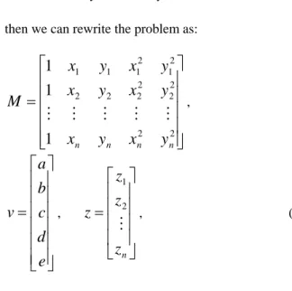
, (1) then we can rewrite the problem as:

⎥

⎦

⎤

⎢

⎣

⎡

=

2 2 2 2 2 2 2 2 2 1 2 1 1 1

1

n n n n

y

x

y

x

y

x

y

x

y

x

y

x

M

,

⎥

⎦

⎤

⎢

⎣

⎡

=

e

d

c

b

a

v

,

⎥

⎦

⎤

⎢

⎣

⎡

=

n

z

M

2 1 , (2)

and then we can get pseudo-inverse for

v

:

z

M

v

=

(

t

)

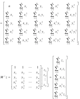
−1 t (3) If there are w*h pixels in the image then n = w*h. For example, if image size is 640 by 480 then n = 307200. If we direct to solve the problem without any numerical method then we have to prepare a very large memory space to store M and the time complexity will be O(n2).

Therefore we have to do some memory reduction and computation speed up in this process. For these reasons, we can combine some repeatable data in the solution procedure. From Equation (2), we know:

⎥ ⎥ ⎥ ⎥ ⎥ ⎦ ⎤ ⎢ ⎢ ⎢ ⎢ ⎢ ⎣ ⎡ ⎥ ⎥ ⎥ ⎥ ⎥ ⎥ ⎦ ⎤ ⎢ ⎢ ⎢ ⎢ ⎢ ⎢ ⎣ ⎡ = 2 2 2 2 2 2 2 1 2 1 2 2 1 1 2 2 2 2 1 2 2 2 2 1 2 1 2 1 1 1 1 1 1 1 n n n n n n n n t y x y x y x y x y x y x y y y x x x y y y x x x M M M M M M M L L L L L

(3)

⎥ ⎥ ⎥ ⎥ ⎥ ⎥ ⎥ ⎥ ⎥ ⎥ ⎥ ⎥ ⎦ ⎤ ⎢ ⎢ ⎢ ⎢ ⎢ ⎢ ⎢ ⎢ ⎢ ⎢ ⎢ ⎢ ⎣ ⎡ = ⎥ ⎥ ⎥ ⎥ ⎦ ⎤ ⎢ ⎢ ⎢ ⎢ ⎣ ⎡ ⎥ ⎥ ⎥ ⎥ ⎥ ⎥ ⎦ ⎤ ⎢ ⎢ ⎢ ⎢ ⎢ ⎢ ⎣ ⎡ = ⎥ ⎥ ⎥ ⎥ ⎥ ⎥ ⎥ ⎥ ⎥ ⎥ ⎥ ⎥ ⎦ ⎤ ⎢ ⎢ ⎢ ⎢ ⎢ ⎢ ⎢ ⎢ ⎢ ⎢ ⎢ ⎢ ⎣ ⎡ =

∑

= = = = = = = = = = = = = = = = = = = = = = = = = = = = = n i i i n i i i n i i i n i i i n i i n n n n n t n i i i n i i n i i n i i i n i i i n i i n i i n i i i n i i n i i n i i n i i i n i i n i i i n i i n i i i n i i n i i i n i i n i i n i i n i i n i i n i i z y z x z y z x z z z z y y y x x x y y y x x x z M y y x y y x y y x x y x x x y y x y y x y y x x y x x x y x y x n 1 2 1 2 1 1 1 2 1 2 2 2 2 1 2 2 2 2 1 2 1 2 1 1 4 2 1 2 1 3 1 2 1 2 2 1 2 1 4 1 2 1 3 1 2 1 3 1 2 1 2 1 1 1 2 1 3 1 1 2 1 1 2 1 2 1 1 1 1 1 M L L L L L

Therefore we only need 30 variables memory space and the time complexity will be O(n) to find the least square sphere fitting algorithm. Figure 5 shows the least square sphere of Figure 1. Figure 6 shows the original image

f(x,y) subtracted by the least square sphere s(x,y) and

then applied contrast stretch. Figure 7 shows the original image f(x,y) compared with the sphere s(x,y) as dynamic threshold process result. Figure 8 shows the number of rice by using connected component algorithm.

Figure 5: The least square sphere fitting of Figure 1.

Figure 6: After removing the background from least

square sphere fitting and then applying contrast stretch of Figure 1.

Figure 7: The original image f(x,y) compared with the

sphere s(x,y) as dynamic threshold process.

Figure 8: Number of rice by using connected

(4)

4. PRINCIPAL POINT OF LENS ON IMAGE PLANE

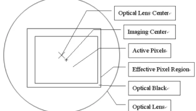
In lens and image sensor assembly or the center of the active pixels of the image sensor, the lens center is not projected to the image plane center shown in Figure 9. If the lens center projected to image plane is

)

y

,

O(x

_o _o , then any lens-related correction image post-processing functions have to shift to O before distortion correction.

Figure 9: The principal point of lens and image.

Lens shading is the reduction in light falling on the image sensor away from the center of the optical axis caused by physical obstructions shown in Figure 10. We can use this phenomenon to find the principal point of lens on the image plane. If we capture a uniform brightness scene, then we can use a spherical surface to fit the image. Also we name the spherical surface as follows. 2 2

)

,

(

x

y

a

bx

cy

dx

ey

f

z

=

+

(4) There is an extreme value on the optical axis therefore we can get the principal point (Cx, Cy) from Equation (5).

e

c

Cy

y

z

d

b

Cx

x

z

2

0

2

0 −

=

∂

−

=

∂

(5)

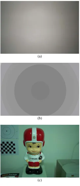
Usually, there is unfavorable non-uniform light falling on the surface causing a gradual brightness gradient in the image. For example, Figure 10 has a slight brightness gradient from bright left to dark right. We

can use the least square plane fitting to suppress this gradual brightness gradient.

For our experiment, lens shading center position is the most robust and quickest way to find the principal point.

(a)

(b)

Figure 10: (a) Lens shading phenomenon. (b) Use lens

shading phenomenon to find the principal point.

5. LENS SHADING COMPENSATION

Lens shading is the reduction in light falling on the image sensor away from the center of the image caused by physical obstructions. The lens shading is one of vignetting of lens [2][4][5]. To suppress the lens shading effect of corner is called the lens shading compensation. The lens shading compensation parameters depend on aperture and focal length [4]. To calibrate the lens shading we can capture a uniform gray card, and record the luminance variation. The basic procedure is shown in Figure 11 and the detailed calibration flow is shown in Figure 12.

(5)

In our calibration we emphasize the lighting distribution on the surface of the calibration pattern. It is very hard to adjust the camera and the calibration pattern without the gradient source lighting induction. The phenomenon is shown in Figures 13, 14, and 15.

(a)

(b)

(c)

(d)

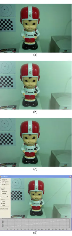
Figure 11: Lens shading calibration procedure. (a)

Capture a uniform brightness scene. (b) Find the normalized radius and illumination relative mapping by using least square mapping. (c) The original image. (d) The lens shading compensated image. It is equal to (c) + (b).

Our lens shading calibration flow is shown in Figure 12.

Figure 12: Lens shading calibration flow. In our

calibration flow we emphasized normalizing the lighting. This is the major difference with other lens shading compensation algorithm.

(6)

(a)

(b)

(c)

Figure 13: (a) A uniform brightness scene. (b) A lens

shading compensation mask without lighting compensation. The compensation mask induces the original lighting effect. (c) A lens shading compensation mask with the lighting compensation.

(a)

(b)

(c)

(7)

(e)

Figure 14: (a) The original scene. (b) Apply Figure 13

(b) lens shading mask result. (c) Apply Figure 13 (c) lens shading mask result. (d) The line profile of luminance of (b) and the dynamic range is 60. (e) The line profile of luminance of (c) and the dynamic range is 15. (a) (b) (c) (d) (e) (f)

(8)

Figure 3.20 (a) The original scene. (b) A uniform

brightness scene with a tilted pose. (c) Apply the lens shading compensation mask from (b) without the lighting compensation. (d) Apply the lens shading compensation mask from (b) with the lighting compensation. (e) The line profile of horizontal of (c) and the dynamic range is 60. (f) The line profile of horizontal of (d) and the dynamic range is 20, which shows much better and uniform brightness.

6. ACKNOLEDGEMENT

This research was supported by the National Science Council of Taiwan, R.O.C., under Grants NSC 92-2213-E-002-072, by the EeRise Corporation, EeVision Corporation, Machvision, Tekom Technologies, Jeilin Technology, IAC, ATM Electronic, Primax Electronics, Arima Computer, and Lite-on.

7. REFERENCES

[1] R. L. Burden and J.D. Faires, Numberical Analysis, 5rd Ed., PWS, Boston, MA, 1993.

[2] S. F. Ray, Applied Photographic Optics, 2rd Ed., Focal Press, Woburn, MA, 1997.

[3] J. C. Russ, The Image Processing Handbook, 3rd Ed., CRC Press, Boca Raton,FL, 1998.

[4] F. Senore, “A Program for Vignetting Correction,” http://www.fsoft.it/Imaging/Vignetting.htm, 2004.

[5] P. van Warlee, “Vignetting,” Version 1.4,

http://www.vanwalree.com/optics/vignetting.html, 2004.