提升高速用戶迴路系統性能之研究

全文

(1)國立交通大學電子工程學系電子研究所. 博士論文. 提升高速用戶迴路系統性能之研究 Performance Enhancement for DMT-based VDSL System: Precursor ISI-Free Frame Synchronization, ISI Cancellation and Optimizing Throughput. 研究生：林尚亭指導教授：魏哲和. 中華民國九十四年七月.

(2) 提升高速用戶迴路系統性能之研究 Performance Enhancement for DMT-based VDSL System: Precursor ISI-Free Frame Synchronization, ISI Cancellation and Optimizing Throughput. 研究生: 林尚亭. Student: Sun-Ting Lin. 指導教授: 魏哲和博士. Advisor: Dr. Che-Ho Wei. 國立交通大學電子工程學系電子研究所博士論文. A Dissertation Submitted to Department of Electronics Engineering & Institute of Electronics College of Electrical Engineering and Computer Science National Chiao Tung University in Partial Fulfillment of the Requirements for the Degree of Doctor of Philosophy in Electronic Engineering July 2005 Hsinchu, Taiwan, Republic of China. 中華民國九十四年七月.

(3) 提升高速用戶迴路系統性能之研究. 研究生: 林尚亭. 指導教授: 魏哲和. 國立交通大學電子工程學系電子研究所. 摘要 DMT (Discrete multitone) 調變技術是目前絕大多數非對稱性用戶迴路 (ADSL)系統所採用的技術，在本論文中，我們首先提出一個觀念，利用增加取樣速度，提升原有非對稱性用戶迴路系統的傳輸速率至高速用戶迴路系統(VDSL)的範圍。同時我們也提出一些演算法來降低信號相互干擾 (ISI)，以提升系統傳輸效能。本論文主要分為三部分，第一部分是有關提升原有非對稱性用戶迴路系統的傳輸速率至高速用戶迴路系統的範圍，要達到這個目標，必須要提高使用頻寛。提高使用頻寛可從二方面進行，一是增大 FFT/IFFT 尺寸，另一方面若維持 FFT/IFFT 大小不變，則需要增加每一個次通道(sub-channel) 的頻寛，為了探討增加頻寛是否改變原有次通道的特性，即每一個次通道內訊號雜訊比變化不能過大，我們針對每一個次通道內訊號雜訊比變化由原本 4 kHz 頻寛依序倍增到 20 kHz 進行分析，同時也針對在不同長度的電話線在各種干擾和雜訊的影響之下，此 i.

(4) 高速用戶迴路系統所能達到的最佳傳輸速率。第二部分則是有關高速用戶迴路系統碼框定位的相關演算法，我們研究一種所謂低複雜度最大可能(low-complexity maximum likelihood)預測演算法，並加以改良，以適合高速用戶迴路系統使用。同時以數學推導証明我們改良的演算法比原有的效能好，因為它能找出傳送資料經過通道影響後真正的碼框起始點，原本的演算法則會因為通道效應影響，後移數個位置到通道強度高峰之處，造成所謂前置信號相互干擾 (precursor ISI)，影響接收端的信號雜訊比。用電腦模擬方式，也可以比較出兩種演算法在接收端的信號雜訊比，我們改良過的演算法表現較佳。第三部分，我們引進一種以遞迴方式，減少殘餘信號相互干擾，降低接收端的數元錯誤率，如此可以減少兩組信號間的防護間隔 (guard interval)，甚至於可以完全不用防護間隔，可提高系統傳輸效能。. ii.

(5) Performance Enhancement for DMT-based VDSL System: Precursor ISI-Free Frame Synchronization, ISI Cancellation and Optimizing Throughput. Student: Sun-Ting Lin. Advisor: Dr. Che-Ho Wei. Department of Electronics Engineering & Institute of Electronics National Chiao Tung University. Abstract Discrete multitone (DMT) modulation is the technology selected for most ADSL systems.. In this dissertation, we proposed a concept to upgrade this DMT-based ADSL. system to the VDSL transmission data rate by increasing the sampling rate. We also proposed algorithms to improve the performance of this DMT-based VDSL system by minimizing the influence of inter-symbol interference (ISI). This dissertation is divided into three parts. In the first part, we try to upgrade the transmission data rate of traditional DMT-based ADSL system to the VDSL range by raising the sampling rate. The sub-channel spacing will grow with the same ratio if the iii.

(6) identical FFT is used. The sub-channel flatness and capacity for VDSL test loops are analyzed by varying the symbol rate from 4 kHz to 20 kHz. In this part, we also investigate the throughput of DMT-based VDSL system at high sampling rates under the influence of various noises/interferences. The throughput limitation of the VDSL system is discussed and the optimal solutions of the sampling rates under various test loop lengths and environment conditions are also investigated. In the second part, a new modified low-complexity maximum likelihood (ML) algorithm for frame synchronization in discrete multitone VDSL transmission system is derived.. Computer simulation results are included to show its improvement in Et/N0. of each tone in the received data. This algorithm estimates the frame boundary at the initial transition edge rather than at the middle peak of a shortened twisted-pair channel response. The timing margin degradation caused by precursor ISI can be reduced significantly, especially when the sub-channels are loaded with more bits. In the third part, an iterative ISI cancellation algorithm is presented to improve the DMT-based VDSL system by canceling the residual ISI outside the guard interval recursively. The guard interval of the system can be shortened to raise the bandwidth efficiency. In addition, by some modifications, the BER performance can be improved significantly even without any guard interval.. iv.

(7) Acknowledgements First of all, I would like to express my sincere gratitude to my advisor, Dr. Che-Ho Wei, for his patient guidance and profound influence down the road to graduate. Special thanks to my friends and colleagues for their genuine encouragement, kind help, etc. Finally, I am deeply indebted to my whole family for their love and supports. This dissertation is dedicated to my grandmother, mother, husband, and daughter. Without their wholehearted care and full support, it is impossible for me to accomplish it.. v.

(8) CONTENTS ABSTRACT .....................................................................................................................I LIST OF TABLES .....................................................................................................VIII LIST OF FIGURES ...................................................................................................... IX GLOSSARY. .............................................................................................................. XI. CHAPTER 1 INTRODUCTION................................................................................ 1 1.1 DMT-BASED ADSL/VDSL SYSTEM ARCHITECTURE ..................................... 5 1.2 TOPOLOGY OF VDSL TEST LOOP ................................................................. 10 CHAPTER 2 CHANNEL MODELING .................................................................. 12 2.1 TRANSMISSION-LINE RLCG CHARACTERIZATION ........................................ 12 2.2 CONVERSION OF RLGC TO ABCD PARAMETERS ......................................... 14 2.2.1 Two-Port Network and ABCD Parameters...................................... 14 2.2.2 ABCD Parameters of Multiple Sections and Bridged-taps ............. 17 2.3 TRANSFER CHARACTERISTICS OF A SUBSCRIBER LOOP ................................ 19 2.4 SIMULATION RESULTS OF THE CHANNEL CHARACTERISTICS ........................ 20 2.5 INTERFERENCE AND NOISE MODELS ............................................................ 23 2.5.1 Crosstalk .......................................................................................... 23 2.5.2 Impulse Noise .................................................................................. 27 2.5.3 Background Noise............................................................................ 28 CHAPTER 3 BIT LOADING AND OPTIMAL THROUGHPUT OF DMT-BASED VDSL SYSTEM.......................................................... 29 3.1 BIT LOADING CALCULATIONS ...................................................................... 30 3.2 CHANNEL CAPACITY VS. SYMBOL RATE OR FFT SIZE .................................. 36 3.3 COMPUTER SIMULATIONS ............................................................................. 39 3.3.1 Maximum Channel Capacity vs. Symbol Rate in AWGN Channel .. 39 3.3.2 AWGN vs. VDSL Noise .................................................................... 42 3.3.3 AWGN vs. Various Crosstalk ........................................................... 43 3.3.4 AWGN vs. Bridged-taps................................................................... 45 3.3.5 Analysis of Maximum Throughput ................................................... 46 3.4 SUMMARY .................................................................................................... 50 CHAPTER 4 FRAME SYNCHRONIZATION BY CYCLIC PREFIX ............... 51. vi.

(9) 4.1 ML ALGORITHM FOR FRAME SYNCHRONIZATION ........................................ 51 4.2 MODIFIED ML ALGORITHM.......................................................................... 54 4.3 COMPUTER SIMULATIONS ............................................................................. 57 4.3.1 Simulation Environment .................................................................. 57 4.3.2 Performance Comparison of ML and Modified ML Algorithms ..... 59 4.3.3 Loop Length and Channel Characteristics...................................... 64 4.3.4 VDSL Test Loops with Complex Topologies .................................... 67 4.4 SUMMARY .................................................................................................... 69 CHAPTER 5 ISI CANCELLATION ALGORITHM FOR DMT-BASED VDSL SYSTEM.............................................................................................. 70 5.1 SYSTEM MODEL ........................................................................................... 71 5.1.1 DMT-based VDSL System................................................................ 71 5.1.2 RISIC Algorithm .............................................................................. 72 5.1.3 Kim’s Approach................................................................................ 74 5.1.4 IIC-ZP Algorithm............................................................................. 76 5.2 COMPUTER SIMULATIONS ............................................................................. 77 5.2.1 Influence of the Residual ISI for a DMT-based System ................... 77 5.2.2 Kim’s Approach and RISIC Performance in DMT-based VDSL System............................................................................................ 81 5.2.3 Performance Comparison of IIC-ZP and RISIC Algorithms........... 83 5.2.4 Residual ISI and Symbol Error Rate................................................ 86 5.3 SUMMARY .................................................................................................... 91 CHAPTER 6 CONCLUSIONS AND FUTURE WORKS ..................................... 92 REFERENCES ............................................................................................................. 95. vii.

(10) List of Tables Table 1.1 VDSL test loops ............................................................................................ 10 Table 1.2 Nominal length for asymmetric VDSL loops ............................................. 10 Table 4.1 ( θ , Et/N0) of VDSL test loops...................................................................... 68. viii.

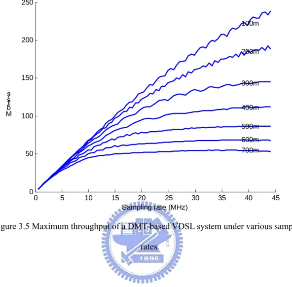
(11) List of Figures Figure 1.1 Discrete multitone line code......................................................................... 6 Figure 1.2 Block diagram of an ADSL transceiver unit-central office (ATU-C). ..... 7 Figure 1.3 Functional block of DMT-based VDSL system.......................................... 8 Figure 1.4 Topologies of VDSL test loops. ...................................................................11 Figure 2.1 Incremental section of twisted-pair transmission line. ........................... 13 Figure 2.2 Two-port network model. .......................................................................... 14 Figure 2.3 A series impedance as a two-port network............................................... 15 Figure 2.4 Two two-port networks in series. .............................................................. 15 Figure 2.5 Example of two-port cascades for twisted-pair line configurations. ..... 17 Figure 2.6 Time domain channel responses of VDSL0 to VDSL7. .......................... 21 Figure 2.7 Frequency domain channel responses of VDSL0 to VDSL7. ................. 21 Figure 2.8 Time domain channel responses of TP1 lines of various lengths. .......... 22 Figure 2.9 Frequency domain channel responses of TP1 lines of various lengths.. 22 Figure 2.10 Illustration of FEXT................................................................................. 25 Figure 2.11 Illustration of NEXT................................................................................. 26 Figure 2.12 Simulation results of the PSD of 10-disturber downstream ADSL NEXT coupling into the upstream as well as ADSL and VDSL FEXT......... 27 Figure 3.1 Channel capacity of gauge #26 twisted-pair line with 8 kHz symbol rate. ............................................................................................................................. 32 Figure 3.2 Averaged PSD flatness of VDSL loops. ..................................................... 35 Figure 3.3 FFT size and symbol rate vs. frequency bandwidth usage. .................... 37 Figure 3.4 Channel capacities of VDSL system with various bandwidths (4.4, 8.8 and 17.6 MHz). .................................................................................................. 38 Figure 3.5 Maximum throughput of a DMT-based VDSL system under various sampling rates.................................................................................................... 40 Figure 3.6 Performance comparison of AWGN with system margin to theoretical one....................................................................................................................... 41 Figure 3.7 Performance comparison of noise type A with AWGN. .......................... 42 Figure 3.8 Performance comparison of noise type B with AWGN........................... 43 Figure 3.9 Performance comparison of HDSL NEXT crosstalk with AWGN......... 44 Figure 3.10 Performance comparison of ADSL NEXT crosstalk with AWGN. ...... 44 Figure 3.11 Performance comparison of VDSL FEXT crosstalk with AWGN........ 45 Figure 3.12 Performance comparison of tested loops with and without bridged-taps. ...................................................................................................... 46 Figure 3.13 (a) Performance and (b) Throughput comparison of tested loop 300 m. ix.

(12) ............................................................................................................................. 47 Figure 3.14 (a) Performance and (b) Throughput comparison of tested loop 600 m. ............................................................................................................................. 48 Figure 3.15 Optimal sampling rate of DMT-based VDSL test loop. ........................ 49 Figure 4.1 Illustration for equation derivation. ......................................................... 56 Figure 4.2 Channel capacity of gauge #26 twisted-pair line with 8 kHz symbol rate. ............................................................................................................................. 60 Figure 4.3 Performance of frame synchronization algorithms with various transmission power (a) -60 dBm/Hz (b) -40 dBm/Hz (c) without AWGN -140 dBm/Hz............................................................................................................... 61 Figure 4.4 SNR difference of various loops. ............................................................... 63 Figure 4.5 Channel response and its SIR of loop VDSL 1200 m. ............................. 64 Figure 4.6 Estimated delays and their Et/N0 vs. window length. ............................. 66 Figure 4.7 θ and Et/N0 of VDSL test loops. ............................................................... 66 Figure 4.8 θ and Et/N0 of VDSL test loops. ............................................................... 68 Figure 5.1 Receiver block for iterative ISI cancellation............................................ 74 Figure 5.2 Block diagram of the Kim’s approach...................................................... 75 Figure 5.3 DMT signal in time domain with one active tone. ................................... 78 Figure 5.4 Received signal with channel length shorter than that of cyclic prefix. 79 Figure 5.5 Received signal with channel length longer than that of cyclic prefix. . 80 Figure 5.6 Bit loading vs. symbol error rate for Kim’s approach. ........................... 81 Figure 5.7 Performance comparison of RISIC (iteration 0) and traditional DMT technology........................................................................................................... 82 Figure 5.8 Performance comparison of RISIC algorithm with different iterations. ............................................................................................................................. 83 Figure 5.9 Performance comparison of DMT, RISIC and IIC-ZP receiver. ........... 85 Figure 5.10 Performance comparison of IIC-ZP receiver with or without TEQ.... 86 Figure 5.11 Channel response for residual ISI influence study. ............................... 87 Figure 5.12 Energy ratio over various cyclic prefix lengths. .................................... 88 Figure 5.13 BER performance of the first iteration IIC algorithm. ........................ 89 Figure 5.14 Corresponding residual ISI energy ratio. .............................................. 89 Figure 5.15 BER performance of the IIC algorithm with one and two iterations.. 90 Figure 5.16 Corresponding residual ISI energy ratio. .............................................. 91. x.

(13) Glossary ADSL. Asymmetric Digital Subscriber Line. ADSL2. Asymmetric Digital Subscriber Line - Second Generation. ADSL2+. Extended Bandwidth ADSL2. ANSI. American National Standards Institute. ATU-C. ADSL Transceiver Unit at Central Office Side. AWGN. Additive White Gaussian Noise. BER. Bit-Error Rate. CAP. Carrierless Amplitude Phase. CO. Central Office. CP. Cyclic Prefix. CPE. Customer Premise Equipment. CSA. Carrier Service Area. DMT. Discrete Multi-Tone. DS. Downstream. DSL. Digital Subscriber Line. ETSI. European Telecommunications Standards Institute. FEQ. Frequency Domain Equalizer. FEXT. Far End Crosstalk. FDD. Frequency Division Duplex. FFT. Fast Fourier Transform. FIR. Finite Impulse Response. HDSL. High Bit Rate Digital Subscriber Line. HDSL2. High Bit Rate Digital Subscriber Line - 2nd Generation xi.

(14) IFFT. Inverse Fast Fourier Transform. IRS. Impulse Response Shortening. ISDN. Integrated Service Digital Network. ITU. International Telecom Union. IIC. Iterative ISI Cancellation. IIC-ZP. Iterative ISI Cancellation with Zero-Padded. ISI. Intersymbol Interference. MMSE. Minimum Mean Square Error. ML. Maximum Likelihood. NEXT. Near End Crosstalk. OFDM. Orthogonal Frequency Division Multiplexing. PSD. Power Spectral Density. QAM. Quadrature Amplitude Modulation. RFI. Radio Frequency Interference. RISIC. Residual ISI Cancellation. SER. Symbol-Error Rate. SIR. Shortened Impulse Response. SISO. Soft Input Soft Output. SNR. Signal to Noise Ratio. TEQ. Time-domain Equalizer. TP. Twisted-Pair. US. Upstream. VDSL. Very-High-Bit-Rate Digital Subscriber Line. VDSL2. Very-High-Bit-Rate Digital Subscriber Line - Second Generation. ZP. Zero-Padding. xii.

(15) Chapter 1 Introduction. In the times before the invention of the telecommunication system, all the information interchange between different places had to be carried by people or other trained animals. Therefore, it is hard to imagine the real-time communication system between separate locations. The invention of telephone systems changes our life style significantly. Although there are various types of telecommunication systems, from the telegraph, telephone, to Internet, their essential function is to provide communication facilities between people from all over the world. With the progress of telecommunication system, the formats of the interchange information include from plain text, real time voices to video, etc., and thus the demand of communication bandwidth explodes dramatically. Due to the rapid development of computer and consumer electronics, traditional telephone subscribers are ready for new services based on digital technologies. There is a lot of accessible information on the Internet, the demands of bandwidth by the residential users drive the digital subscriber loop (DSL) systems to become more mature. There are two candidates for the Internet networks: cable modem provided by cable TV companies, or DSL system provided by traditional telecommunication companies. The details of performance comparisons between these two systems are not covered in this dissertation. In summary, each of them has its advantages and limitations. However, the 1.

(16) DSL system is much more popular in Taiwan because most last-mile twisted-pair telephone wires are short enough for the DSL system to be operated. In addition, the Chung-Hwa Telecommunication company has been very active to establish the DSL network and promote the DSL service since the very beginning. Actually, the DSL technology has been studied earlier to improve the bandwidth efficiency of the twisted-pair lines, but it is not attended to until the population of the Internet becomes very large. Since the end user usually attend to download or browse a lot of data from the Internet, the technology called asymmetric DSL (ADSL) is selected by most traditional telecommunication company to provide the Internet services. The ADSL system was developed for video-on-demand services since 1991 with a high transmission throughput from a central office to telephone subscribers downstream [1]. The first generation ADSL standards are capable of a downstream transmission throughput of 6.433 Mbits/s over carrier serving area (CSA) distance. For longer telephone subscriber loops confirming the resistance design rule, the downstream transmission throughput is reduced to 1.544 Mbits/s. Discrete Multi-Tone (DMT) modulation is the ADSL modem standard approved by ANSI [2]. But DMT is being challenged by the other technology known as Carrierless Amplitude Phase (CAP) modulation. Both systems work very well, according to users at telephone companies that are trialing ADSL before they market the services. There are many discussions on the other advantages/disadvantages of CAP vs. DMT. A reasonably impartial summary of these is [3]: 1. DMT can direct information to sub-carriers and modulate them independently. CAP has a single carrier which has to be treated as a whole, even though channel characteristics vary widely. As a result, DMT may deliver better performance or be more spectrally efficient (i.e., for standard ADSL, DMT only needs roughly two-thirds the bandwidth of CAP). 2.

(17) 2. DMT is more complex to initialize and needs more power-up time than CAP. 3. DMT is inherently and straightforwardly rate-adaptive. It delivers the maximum data for any given line. This allows the support of higher rates over shorter loops (8 Mbits/s), or sub-rate connections at very long reach. CAP can support rate adaptation by varying the constellation and the bandwidth, but it requires very careful analog design, and the rates have much lower granularity. DMT steps in 32 kbits/s steps from 64 kbits/s to 8 Mbits/s vs. CAP's 320 kbits/s steps from 320 kbits/s to 7 Mbits/s. 4. DMT has much greater latency; this may actually infringe some specifications for special services such as ISDN. 5. CAP is more resistant to RFI, although DMT can be more adept at coping with multiple or varying RFI sources. 6. CAP has a lower peak-to-average ratio which simplifies the design of the analog stage. and. reduces. its. power. needs. for. a. given. bandwidth. and. power-spectral-density. 7. It is simple for DMT to meet an arbitrary or variable power mask spectrum for spectral compatibility. 8. Echo-cancellation in DMT is more difficult. 9. Because its symbols are longer, DMT has greater immunity to impulse noise than CAP. 10. CAP can be easier to optimize to a specific application. DMT can be more complex, but it supports more versatility and flexibility. This is important in ADSL with many applications and a wide range of environments. 11. DMT's analysis and measurement functions can be used for diagnostics and testing to detect out-of-specification systems or for preventive maintenance of the copper lines. 3.

(18) Bellcore (with Bell Telephone and Nynex) organized the “ADSL Olympics” to evaluate and compare three line code contenders from 1993. Trial results indicated that DMT had performed better than CAP and QAM (Quadrature Amplitude Modulation). Consequently, although not unanimously embraced, both ANSI (for the USA) and ETSI (for Europe) adopted DMT, and ANSI T1.413 [2] was born. The standard today is endorsed by the ITU. When we began our research of ADSL transceiver from 1998, DMT-based ADSL system has been popular since it is superior in dealing with line impairments. DMT has since been widely deployed, and proven its value as a successful line-coding approach, therefore, we focus to study and improve the DMT-based ADSL system at first. Although the transmission throughput of the ADSL system is much more than the traditional dial-up modem (only up to 56 kbits/s), it still needs to be improved to provide more advanced broadband multimedia services. Due to the population increase of fiber on the telecommunication network, the length of twisted-pair line as the last-mile can be gradually reduced. The available frequency spectrum of these short copper wires for transmission becomes much broader and its optimal data rate grows dramatically. A service called very-high-speed DSL (VDSL) [4][5][6][7] has been under study since late 1995, which can provide up to 52 Mbits/s over short telephone line, to meet the requirements for broadband access-network. VDSL can be regarded as an evolution of the ADSL system, which uses the frequency band from a few hundred kilohertz to beyond 10 MHz on some loops. The standard of VDSL system is under study at ITU-T, ANSI [4], and ETSI at 1998, it is desirable to construct a solution that can support either symmetric or asymmetric transmission. Although the ADSL system was mature in the commercial applications at that time, there are some issues to improve their performance closer to their line capacity limits, such as frame synchronization approach, reducing the inter-symbol interference (ISI) and to increasing the data transmission rate, etc. From those studies, we found a method to extend 4.

(19) the data transmission rate and then improve the DMT-based ADSL system to the performance of VDSL system by increasing the sampling rates. Based on this concept, we proposed a DMT-based VDSL system similar to the structure of the traditional DMT-based ADSL one. In this dissertation, the performance of DMT-based VDSL system is investigated. The system architecture is introduced at first and then the channel response modeling of the DSL environment is derived in Chapter 2. Chapter 3 is the bit-loading capacity for various channels under different environments. In Chapter 4, a low-complexity frame synchronization method is applied to the DMT-based VDSL system, and a modified approach is also proposed to improve the performance of the whole system. From these studies, it is found that the ISI effect causes serious problem to the whole system. Then an iterative ISI cancellation algorithm for the DMT-based VDSL system is presented in Chapter 5.. 1.1 DMT-based ADSL/VDSL System Architecture DMT modulation is a technique in which a transmission channel is partitioned into a number of independent, parallel sub-channels, and each of them carries a lower-speed QAM signal, as shown in Fig. 1.1 [8]. In wireless applications, it is denoted as orthogonal frequency division multiplexing (OFDM) system [9]. The same modulation scheme is also used in the twisted-pair copper lines for data transmission, this application is denoted as DMT-based ADSL system [1].. 5.

(20) POTS. 1.1 MHz 4 KHz e.g. 128-QAM. Data rate = Number of sub-channels x number of bit/sub-channel x modulation symbol rate Figure 1.1 Discrete multitone line code. From the study of the DMT-based ADSL system, some modifications that can improve the performance of whole system are proposed in this dissertation. These enhancements even can uplift the optimal bit rate to the range of VDSL system by extending the frequency bandwidth. After these ideas are presented in the 2001 IEEE Globecom conference [10], a new system called ADSL2+ [11][12] using double bandwidth was proposed in 2003, which is just similar to our proposed DMT-based VDSL system. In this dissertation, we propose an asymmetric VDSL system, which is upgraded from a DMT-based ADSL system by doubling the sampling rate but remaining the same structure of the DMT symbol. The VDSL system described in this dissertation is asymmetric with a architecture similar to the ADSL system, as shown in Fig. 1.2 [2]. In this dissertation, we focus on improving the system performance involving modulation, synchronization block, but not the coding parts. The simplified functional blocks of the DMT-based DSL system, including path, noise, transmission and receiver side, are shown in Fig. 1.3.. 6.

(21) Figure 1.2 Block diagram of an ADSL transceiver unit-central office (ATU-C). 7.

(22) r0. N(t) r(t). P(t). TEQ. z0 rL. FFT + FEQ. s(t). Serial-to-Parallel. yk. Parallel-to-Serial. xk. IFFT. DMT Symbol Generator. y0. x0. H(t) xN-1. yN-1. Frame Synchronizer. rN+L-1. zN-1. Figure 1.3 Functional block of DMT-based VDSL system.. The maximum transmission data rate supported by this system depends on the characteristics of channel. Therefore, the channel modeling and bit-loading of each sub-channel should be computed. The DMT generator can organize random data into DMT symbols according to these parameters such as the bit-loading of each sub-channel and pilot tone, synchronization symbol, etc. The performance of frame synchronization algorithm is monitored and is measured by calculating the differences between received data and the original one. The output data of DMT generator, xk, are used to modulate N sub-carriers by using an inverse Fast Fourier transform (IFFT) to yk, and the last L samples are copied and put as cyclic prefix to form a frame sk. P(t) is the channel impulse response of twisted-pair line applied, and H(t) is the transfer function of the system including noise and time-domain equalizer (TEQ). The received data, r(t) is the convolution of s(t) and H(t). In the receiver, after detecting the frame boundary, the first L samples are discarded and the remaining N samples are demodulated by a FFT. A frequency domain equalizer (FEQ) is also applied to 8.

(23) compensate the channel dispersion. The transmission channel modeling of the twisted-pair lines has played an important role in the engineering of DSL systems. Two sets of test loops employed in this dissertation will be discussed in detail in section 1.2. The transmission characteristics of these worst-case loops are then simulated with channel impulse responses derived from twisted-pair cable primary parameters. Most twisted-pair phone lines can be well-modeled for transmission at frequencies up to 30 MHz by using the well-known two-port modeling or “ABCD” theory [1][13][14]. The procedure for generating the channel modeling includes transmission-line RLCG characterization, RLGC to ABCD parameters conversion, multiple ABCD section integration, and transfer characteristics of a subscriber loop calculations. According to the parameters and equations mentioned in [15], we have developed a set of MATLAB programs to generate the channel modeling of the twisted-pair lines. The DMT technique applied to a transmission line can be viewed as a set of independent frequency-indexed sub-channels with center frequency fi. Each sub- channel is approximately flat that no transmission distortion is evident, and the overall capacity is the summation of the sub-channels. The number of bits per symbol carried by the ith tone (sub-channel) can be calculated using the formula given in reference [1].. 9.

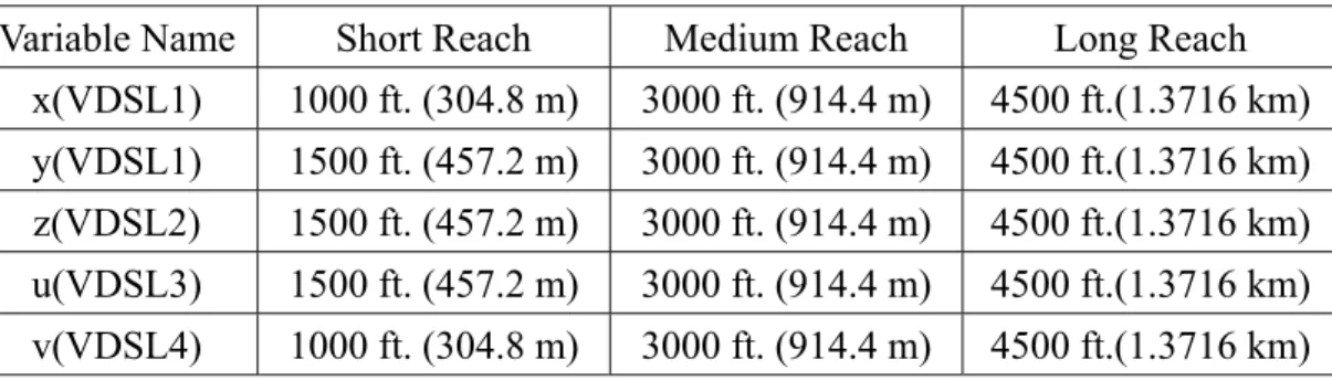
(24) 1.2 Topology of VDSL Test Loops There are 8 test loop topologies listed in the VDSL draft standard, namely, from VDSL0 to VDSL7, and their purposes of test are summarized in Table 1.1 while their topologies are shown in Fig. 1.2. Table 1.2 enumerates short, medium, and long-range values for a nominal length variable in VDSL1 through VDSL4 [4]. In order to study the effect of loop length to the whole system, anther set of loops with length from 100 m to 1500 m is the second test set. In this section, the DMT-based DSL system description and topology of VDSL test loops are introduced. The characteristics of these twisted-pair lines can be modeled by a mathematical method described in the next section. Table 1.1 VDSL test loops No.. Rationale. VDSL0. Null loop. VDSL1. Range stress limit, underground cable. VDSL2. Flat-wire vertical drop, horizontal aerial cable on other section. VDSL3. Reinforced-wire vertical drop, horizontal aerial cable on other section. VDSL4. Bridged tap, horizontal aerial cable. VDSL5. Short loop test with bridged taps and various crosstalk. VDSL6. Medium loop test with bridged taps and various crosstalk. VDSL7. Long loop test with bridged taps and various crosstalk. Table 1.2 Nominal length for asymmetric VDSL loops Variable Name. Short Reach. Medium Reach. Long Reach. x(VDSL1). 1000 ft. (304.8 m). 3000 ft. (914.4 m). 4500 ft.(1.3716 km). y(VDSL1). 1500 ft. (457.2 m). 3000 ft. (914.4 m). 4500 ft.(1.3716 km). z(VDSL2). 1500 ft. (457.2 m). 3000 ft. (914.4 m). 4500 ft.(1.3716 km). u(VDSL3). 1500 ft. (457.2 m). 3000 ft. (914.4 m). 4500 ft.(1.3716 km). v(VDSL4). 1000 ft. (304.8 m). 3000 ft. (914.4 m). 4500 ft.(1.3716 km). 10.

(25) FP flat untwisted pair TP1 0.4mm or 26-gauge TP2 0.5mm or 24-gauge TP3 DW10. VDSL0 VDSL1 VDSL2. VDSL3. 2m TP2. x(=305/913/1372m) TP1 76.2m FP. z-76.2 m TP2. 76.2m TP3. u-76.2m TP2. S4_2 = 91.4m, S4_3 = 45.7m, S5_2 = 15.2m TP2. VDSL4. S4_2. v-91.4m TP1. S4_3. S5_2. 167 m 30.4m 76.2m. VDSL5. TP2. 503m. VDSL6. VDSL7. TP1. TP2. TP2. 198m VDSL5. TP2. 503m. 701m. TP1. TP2. VDSL5. Figure 1.4 Topologies of VDSL test loops.. 11.

(26) Chapter 2 Channel Modeling. Most twisted-pair phone lines can be well-modeled for transmission at frequencies up to at least 30 MHz by using what is known as two-port modeling or “ABCD” theory [1][13][14][15][16]. The procedure for generating the channel modeling includes transmission-line RLCG characterization, RLGC to ABCD parameters conversion, multiple ABCD section integration, and transfer characteristics of a subscriber loop calculations, etc. In this chapter, the basic theory of the channel modeling and their computer simulation results are included as well as the relative noise models such as crosstalk and background noises are introduced in this chapter.. 2.1 Transmission-line RLCG Characterization The R, L, C, and G parameters represent resistance, inductance, capacitance, and conductance per unit length of the transmission line, respectively. The two-port characterization of a transmission line can be derived from the per-unit length two-port model in Fig. 2.1.. 12.

(27) I(x). I(x+dx). Rdx. Ldx. V(x). V(x+dx). Cdx Gdx. Figure 2.1 Incremental section of twisted-pair transmission line.. The RLCG can be fitted to the measured values which are frequency dependent. The other coefficients in the models are related to the types of twisted-pair lines and can be looked up in reference [1][14]. The curve-fitting RLCG values are listed as 1. R( f ) =. 1 4. L( f ) =. r04c + ac × f 2. l0 + l∞ × ( f / f m )b 1 + ( f / f m )b. C ( f ) = c∞ + c0 ⋅ G( f ) =. 1. + 4. ……………………………………..(2.1). r04s + as × f 2. ………………………………………………………….(2.2). − f ce ……………………………………………………………..(2.3). + g 0 ⋅ f g e ………………………………………………………………….(2.4). where r0c (kΩ/kft) is the copper-line DC resistance; ac is characterizing the rise of resistance with frequency in the “skin” effect; l0 (mH/kft) and l∞ (mH/kft) are the lowand high- frequency inductance, respectively; f (MHz) is the frequency at which R and L are calculated; fm (MHz) and b are characterizing the transition between low and high frequencies in the measured inductance values. In this section, the transmission-line RLCG characterization is defined and the curve-fitting formulae of the RLCG parameters for twisted-pair line are also introduced. These parameters can be converted to ABCD matrix parameters.. 13.

(28) 2.2 Conversion of RLGC to ABCD Parameters In this section, we introduce how to convert the RLGC to ABCD parameters and the multiple ABCD section integration.. 2.2.1 Two-Port Network and ABCD Parameters. I1 V1. I2 A B C D. V2. Figure 2.2 Two-port network model.. Fig. 2.2 shows a transmission model of two-port linear circuit. The terminal voltages and currents will be defined by the matrix relationship given by. ⎡V 1⎤ ⎡ A B ⎤ ⎡V 2 ⎤ ⎡ ⎤ ⋅ ⎢ ⎥ = Φ ⋅ ⎢V 2 ⎥ …………………………………………………….(2.5) ⎢ ⎥=⎢ ⎥ ⎣ I 1 ⎦ ⎣C D ⎦ ⎣ I 2 ⎦ ⎣ I2⎦ Where Φ is a 2x2 matrix of 4 possibly frequency-dependent parameters, A, B, C, and D. All these parameters depend only on the network and not on external connections. For example, ABCD parameters for a simple two-port network consisting of a series impedance, as shown in Fig. 2.3, can be derived as follows. ⎡ A B ⎤ ⎡1 Z ⎤ ⎢C D ⎥ = ⎢0 1 ⎥ …………………………………………………………………….(2.6) ⎦ ⎦ ⎣ ⎣. 14.

(29) I2. I1 Z. V1. V2. Figure 2.3 A series impedance as a two-port network.. I2. I1 V1. N1. I3. I2 V2. V2. N2. V3. Figure 2.4 Two two-port networks in series.. The ABCD parameters of two two-port networks in series can be obtained by equating the voltage and current of the first two-port network to that of the following network, as shown in Fig. 2.4. For two two-port networks in series, the input and output voltage and current relationship is represented as follows. ⎡V1 ⎤ ⎡ A1 ⎢ I ⎥ = ⎢C ⎣ 1⎦ ⎣ 1. B1 ⎤ ⎡V2 ⎤ D1 ⎥⎦ ⎢⎣ I 2 ⎥⎦. ⎡V2 ⎤ ⎡ A2 ⎢ I ⎥ = ⎢C ⎣ 2⎦ ⎣ 2. B2 ⎤ ⎡V3 ⎤ D2 ⎥⎦ ⎢⎣ I 3 ⎥⎦. and ⎡V1 ⎤ ⎡ A1 ⎢ I ⎥ = ⎢C ⎣ 1⎦ ⎣ 1. B1 ⎤ ⎡ A2 D1 ⎥⎦ ⎢⎣C 2. B2 ⎤ ⎡V3 ⎤ …………………………………………………….(2.7) D2 ⎥⎦ ⎢⎣ I 3 ⎥⎦. 15.

(30) To derive the relationship between “RLCG” and “ABCD” parameters, some new variables have to be introduced. First, the impedance per unit length, Z, is defined as R+jwL and the admittance per unit length, Y, is G+jwC. By taking equations (2.6) and (2.7) into Fig. 2.1, the ABCD parameters of a unit-length twisted-pair line are expressed by. ⎡V ( x ) ⎤ ⎡1 Z ⎤ ⎡ 1 0 ⎤ ⎡V ( x + dx ) ⎤ ⎡ A B ⎤ ⎡V ( x + dx ) ⎤ ⎢ ⎥=⎢ ⎥=⎢ ⎥ ………………………..(2.8) ⎥⎢ ⎥⎢ ⎥⎢ ⎣ I ( x ) ⎦ ⎣0 1 ⎦ ⎣Y 1 ⎦ ⎣ I ( x + dx ) ⎦ ⎣C D ⎦ ⎣ I ( x + dx ) ⎦. The incremental section of twisted-pair transmission line is calculated by evaluating the voltage and currents at x=0 in terms of those at x=d. The following two-port representation is then obtained [4].. Z 0 ⋅ sinh(γd )⎤ ⎡ cosh(γd ) ⎡V(0)⎤ ⎢ ⎥ ⋅ ⎡V(d)⎤ 1 = ⎥ ⎢ ⎢ cosh(γd ) ⎥ ⎢ I(d) ⎥ ………………………………………(2.9) ⋅ sinh(γd ) ⎦ ⎣ I(0) ⎦ ⎢ Z ⎣ ⎣ 0 ⎦⎥. where the propagation constant γ and characteristic impedance Z0 of the transmission line are defined, respectively, by γ = Z0 =. (R + jwL )⋅ (G + jwC ) =. (R + jwL ) (G + jwC ). =. Z ⋅ Y …………………………………………………..(2.10). Z Y …………………………………………………………….(2.11). The “ABCD” parameters are related to the propagation constant γ , characteristic impedance Z0, and length of a transmission line d. However, a subscriber loop is usually constructed by combining several different lines. In the next section, multiple ABCD section integration and the characteristics of bridged-tap are introduced. 16.

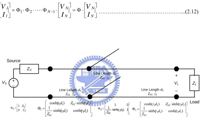
(31) 2.2.2 ABCD Parameters of Multiple Sections and Bridged-taps Since the ABCD matrix of a composite network consisting of two-port networks in series is obtained by the product of these two ABCD parameters matrices as shown in equation (2.7). A cascade of two-port networks has an equivalent two-port matrix that is the product of the component ABCD matrices, in order, as shown by. ⎡V N ⎤ ⎡V N ⎤ ⎡V 1⎤ ⎥ = Φ⋅⎢ ⎥ ………………………………………...(2.12) ⎢ ⎥ = Φ1 ⋅ Φ 2 ⋅ L ⋅ Φ N −1 ⋅ ⎢ ⎣ I1⎦ ⎣IN⎦ ⎣IN⎦. Source ZS Line Length d2 Z02 , γ2. + –. VS. VL Line Length d3 Z03 , γ3. Line Length d1 Z01 , γ1 ⎡1 ZS ⎤ Φ0 = ⎢ ⎥ ⎣⎢0 1 ⎦⎥. +. ⎡ cosh(γ1d1) Z01⋅sinh(γ1d1)⎤ ⎥ Φ1 = ⎢ 1 ⎢ ⋅ sinh(γ1d1) cosh(γ1d1) ⎥ ⎣Z01 ⎦. ⎡ 1 0⎤ Φ2 = ⎢ 1 ⋅ tanh(γ d ) 1⎥ ⎢ ⎥ 2 2 ⎢⎣ Z02 ⎦⎥. ZL. –. Z03 ⋅ sinh(γ 3d3)⎤ Load ⎡ cosh(γ 3d3) ⎢ ⎥ Φ3 = 1 cosh(γ 3d3 ) ⎥ ⎢ ⋅ sinh(γ 3d3 ) ⎣ Z03 ⎦. Figure 2.5 Example of two-port cascades for twisted-pair line configurations.. Another more general configuration of loops with bridged-taps and various types of twisted-pair lines is shown in Fig. 2.5. The transmission matrix can be expressed as. ⎡V S ⎤ ⎡V L ⎤ ⎡V L ⎤ = Φ ⋅ Φ ⋅ Φ ⋅ Φ ⋅ = Φ ⋅ ⎢ ⎥ ⎥ ⎢ ⎥ ……………………..………(2.13) 0 1 2 3 ⎢ ⎣IL⎦ ⎣IL⎦ ⎣IS⎦ where 17.

(32) ⎡1 Z s ⎤ Φ0 = ⎢ ⎥ ……………………………………………………………...………..(2.14) ⎣0 1 ⎦. Z 01 ⋅ sinh(γ 1d1 ) ⎤ ⎡ cosh(γ 1d1 ) ⎢ ⎥ Φ1 = 1 ⎢ ⎥ ⋅ sinh(γ 1d1 ) cosh(γ 1d1 ) ……………………………………….…..(2.15) ⎣⎢ Z 01 ⎦⎥. 1 0⎤ ⎡ ⎥ ……………………………………………..…..……(2.16) Φ 2 = Φt = ⎢ 1 ⎢ ⋅ tanh(γ 2 d 2 ) 1 ⎥ ⎢⎣ Z 02 ⎥⎦. Z 03 ⋅ sinh(γ 3d3 ) ⎤ ⎡ cosh(γ 3 d3 ) ⎥ Φ3 = ⎢ 1 ⎢ ⎥ ⋅ sinh(γ 3 d3 ) cosh(γ 3 d3 ) ………………………………...…….….(2.17) ⎢⎣ Z 03 ⎥⎦ where Zs is the source impedance and Zt is the characteristic impedance of the bridged-tap section. The impedance of the bridged-tap section Zt is computed according to the above formula, as a parallel (shunt) impedance, for the input impedance of a section of transmission line terminated with an open circuit (ZL= ∞ ). The overall two-port matrix is simply the product of the 4 two-port matrices shown in Fig. 2.5 and equations (2.13) to (2.17). Circuits with multiple bridge-taps can be calculated by similar procedures as multiplying multi-section of two-port networks. The impedance of previous section then becomes a termination impedance for the next section working backwards towards the main transmission pair of interest. The calculation process is straightforward and recursive to build the whole loop models.. 18.

(33) 2.3 Transfer Characteristics of a Subscriber Loop The computation of the transfer functions for twisted-pair transmission lines with multiple sections then simply becomes a process of multiplying the corresponding ABCD matrices of the cascaded two-port sections. The source voltage divider is modeled by equation (2.18) and the final output voltage, current and load are VL, IL, and ZL, respectively. The transfer function, H, is computed from the ratio of VL and Vs, as shown in equation (2.19).. H( f ) =. VL Z1 = ⋅ T ( f ) ……………………………………………………….....(2.18) Vs Z s + Z1. , where T(f) is the ratio of VL and V1, and. T( f ) =. Z1 = Z 0. H( f ) =. 1 …………………………………………...(2.19) Z cos(γ d ) + ( 0 ) ⋅ sinh(γ d ) ZL Z L + Z 0 ⋅ tanh(γ d ) …………………………………………………….(2.20) Z 0 + Z L ⋅ tanh(γ d ). Z 0 ⋅ sec h(γ d ) ⎡ Z0 ⎤ ⎡ Z0 ⎤ …………………..(2.21) Z s ⋅ ⎢ + tanh(γ d ) ⎥ + Z 0 ⋅ ⎢ + tanh(γ d ) ⎥ ⎣ ZL ⎦ ⎣ ZL ⎦. In DSL case, the source impedance is matched to the characteristic impedance (which equals the input impedance of the line when the line is long) and all impedances are real over the higher frequency range for DSL transmission. In this case, the transfer function is simply 6 dB lower than the insertion loss. The transfer function, H, is called the channel modeling of a twisted-pair line. Usually, its form can be represented both in frequency-domain and time-domain by applying proper sampling time. A program to. 19.

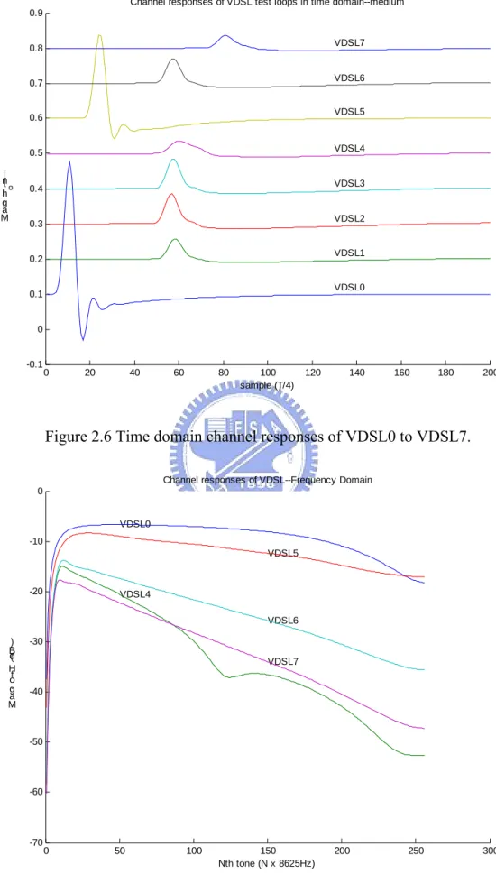
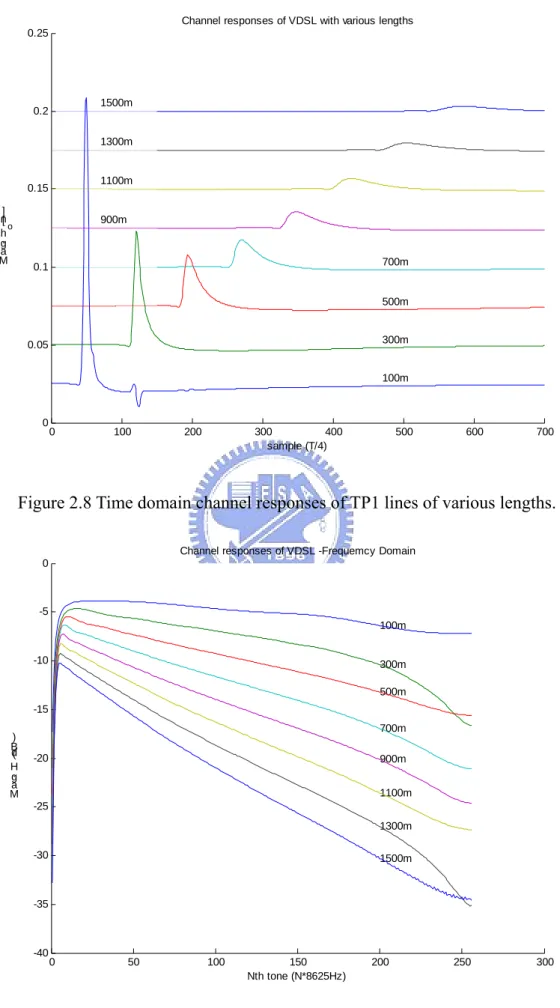
(34) generate the time- domain transfer function of xDSL implemented according to the theory mentioned above is developed, and some of the results used in VDSL are shown in the next section.. 2.4 Simulation Results of the Channel Characteristics In this section, some simulation results of the DSL channel characteristics will be illustrated. In the first test set, the VDSL test loops, VDSL0 to VDSL7 in Table 1.1, Table 1.2, and Fig. 1.4 in Chapter 1 are studied. The other test set is the TP1 (gauge #26) line with length from 100 m to 1500 m since the VDSL system limits its twisted-pair loop length up to 1500 m. This set of test loops is simulated to observe the relationship between channel characteristics and its length. In Fig. 2.6 and 2.7, the channel responses of VDSL0 to VDSL7 of short reach in Table 1.2 (about 300 to 450 m) are illustrated in both time-domain and frequency-domain. While the channel responses of the second test set are shown in Fig. 2.8 and Fig. 2.9. From the simulation results, it can be seen that the time-domain channel response of VDSL4, which has two bridged-taps, contains several peaks, with a broader main peak. In addition, its frequency-domain channel response contains some notches. The SNR values at those notches are reduced and the number of bits carried are also decreased. In general, the longer the loop, the broader the response will be. In addition, the delay becomes greater while the loop length gets longer.. 20.

(35) Channel responses of VDSL test loops in time domain--medium 0.9 VDSL7. 0.8. VDSL6. 0.7. VDSL5. 0.6. VDSL4. 0.5 ] n[ o h g. a M. VDSL3. 0.4. VDSL2. 0.3. VDSL1. 0.2. VDSL0. 0.1. 0. -0.1. 0. 20. 40. 60. 80. 100 sample (T/4). 120. 140. 160. 180. 200. Figure 2.6 Time domain channel responses of VDSL0 to VDSL7. Channel responses of VDSL--Frequency Domain 0 VDSL0 -10 VDSL5. -20. VDSL4 VDSL6. ) B d( H f o g. a M. -30 VDSL7 -40. -50. -60. -70. 0. 50. 100. 150 Nth tone (N x 8625Hz). 200. 250. 300. Figure 2.7 Frequency domain channel responses of VDSL0 to VDSL7. 21.

(36) Channel responses of VDSL with various lengths 0.25. 1500m. 0.2. 1300m. 1100m. 0.15 ] n[ o h g. a M. 900m. 700m. 0.1. 500m. 300m. 0.05. 100m. 0. 0. 100. 200. 300 400 sample (T/4). 500. 600. 700. Figure 2.8 Time domain channel responses of TP1 lines of various lengths. Channel responses of VDSL -Frequemcy Domain 0. -5 100m -10. 300m 500m. -15 ) B d( H g. a M. 700m -20. 900m 1100m. -25 1300m -30. 1500m. -35. -40. 0. 50. 100. 150 Nth tone (N*8625Hz). 200. 250. 300. Figure 2.9 Frequency domain channel responses of TP1 lines of various lengths. 22.

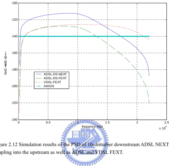
(37) 2.5 Interference and Noise Models In the above sections, the channel responses of the twisted-pair lines are derived. However, in the real DSL operating environment, there are other effects, such as crosstalks, noises, etc. that will lower the performance of the DSL system. Besides the natural limitation of thermal noise, there are three other types of interference or noise that affect the performance of DSL system, i.e., crosstalk [17][18][19][20][21][22][23], impulse noise [17][24][25][26], and background noise [1].. 2.5.1 Crosstalk Telephone subscriber loops are organized in bundle groups of 10, 25, or 50 pairs, and several binder groups share a common physical shield in a cable. Due to capacitive and inductive coupling, there is crosstalk between the twisted-pair lines even though pairs are well insulated at DC. For DSL system, in which the signal bandwidth is much broader than that of voice frequency, the crosstalk becomes a dominant limitation to the whole transmission throughput. Crosstalk coupling loss models have been developed for far end crosstalk (FEXT) [19] and near end crosstalk (NEXT) [18][20][21] with the consideration of different number of disturbers. These crosstalk coupling loss models are based on twisted-pair lines within the same cable of significant length, usually longer than 300 m. The effect of crosstalk could be different if only a portion of twisted-pair lines are within the same cable. In this subsection, the formula of power spectrum density (PSD) of ADSL downstream are introduced and their induced FEXT and NEXT to the system are also discussed and simulated. 23.

(38) 2. PSDADSL-Disturber. ⎡ ⎛ π f ⎞⎤ ⎢sin ⎜ ⎟⎥ 2 ⎣ ⎝ fo ⎠ ⎦ …..(2.22) = K ADSL × × × | LPF ( f ) |2 × | HPF ( f ) |2 , 0 ≤ f < ∞ 2 fo ⎛π f ⎞ ⎜ ⎟ ⎝ fo ⎠. , where f0=2.208 × 106Hz, KADSL= 0.1104 Watts. This equation gives the single sided PSD, where KADSL is the total transmitted power in Watts for the downstream ADSL transmitter before shaping filters, and is set such that the ADSL PSD will not exceed the maximum allowed PSD. f0 is the sampling frequency in Hz.. f hα 36 LPF ( f ) = α , f h = 1.104 × 10 6 Hz , α = = 11.96 ……………(2.23) α 10 log(2) f + fh 2. LPF is a low pass filter with a 3 dB point at 1104 kHz and 36 dB/octave rolloff.. 2. HPF ( f ) =. f α + f lα , f l = 4000 Hz , f h = 25875 Hz , α = f α + f hα. 57.5 f 10 log h fl. = 7.09 ……...….(2.24). HPF is a high pass filter with 3 dB points at 4 kHz and 25.875 kHz and 57.5-dB attenuation in the voice band, separating ADSL from POTS. With this set of parameters the PSDADSL-Disturber is the PSD of a downstream transmitter that uses all the sub-carriers.. A. FEXT Coupling Configurations. FEXT [1][2][19] is defined as the crosstalk effect between a receiving path and a transmitting path of DSL transceiver at opposite ends of two different subscriber loops within the same twisted-pair cable, as shown in Fig. 2.10.. 24.

(39) Pair i Signal source. Disturbed, far end FEXT Disturbing, far end. Pair j. Figure 2.10 Illustration of FEXT.. The FEXT loss model is given by [2]. 2. 2. H FEXT ( f ) = H channel ( f ) × k × l × f 2 ……………………………………….(2.25) where Hchannel (f) is the channel transfer function, k is the coupling constants, l is the −20 0.6 for n<50, 1% coupling path length and f is the frequency. k is 8.0 ×10 × (n / 49). worst-case disturbers with the coupling path length l in feet. If the meter of length is used, −20 0.6 then the coupling constant k is changed to 2.44 ×10 × (n / 49) for n<50.. The FEXT noise PSD is therefore given by. 2. PSD ADSL − FEXT = PSD ADSL − Disturber × H FEXT ( f ) ……………………...………..(2.26) In Fig. 2.12, the magnitude of these FEXT noises are shown in frequency domain.. B. NEXT Coupling Configurations. NEXT [1][2][18][19] is defined as the crosstalk effect between a receiving path and a transmitting path of DSL transceivers at the same end of two different subscriber loops with in the same twisted-pair cable, as shown in Fig. 2.11.. 25.

(40) Signal source. Pair i. Disturbed, near end. Pair j. Disturbing, near end. NEXT. Figure 2.11 Illustration of NEXT.. The PSD of the ADSL NEXT coupling into the upstream is defined as [2]. (. PSD ADSL − NEXT = PSD ADSL − Disturber × x n × f 3 / 2 where. ). for 0 ≤ f < ∞, n < 50 ………..(2.27). xn = 8.818 ×10−14 × (n / 49)0.6 or equivalently, xn = 0.8536 ×10−14 × n0.6 . The. integration of the induced NEXT over the band from 0 to 1.104 MHz for n=49 is –25.4 dBm.. Fig. 2.12 shows the simulation results of the PSD of 10-disturber downstream ADSL NEXT into the upstream as well as ADSL and VDSL FEXT with 300 m loop length.. 26.

(41) -100. -120. -140. ) Z H/ m B d( D S P. -160. -180 ADSL-DS-NEXT ADSL-DS-FEXT VDSL-FEXT AWGN. -200. -220. -240. 0. 0.5. 1. 1.5 frequency (Hz). 2. 2.5 6. x 10. Figure 2.12 Simulation results of the PSD of 10-disturber downstream ADSL NEXT coupling into the upstream as well as ADSL and VDSL FEXT.. 2.5.2 Impulse Noise The origin of impulse noise is usually difficult to locate. It could come directly through some connections to the telephone subscriber loop or come from the influence of an electromagnetic field. Impulse noise is characterized as a random pulse waveform whose amplitude is much higher compared with the Gaussian-like background noise. Impulse noise is a major impairment for DSL system, especially due to the heavy DSL subscriber loop loss. While crosstalk and background noises impose a limit on transmission throughput over the twisted-pair telephone subscriber loop, the error caused by impulse 27.

(42) noise can be corrected with forward error correction codes. The required error correction coding overhead could reduce a small portion of the transmission throughput.. 2.5.3 Background Noise The loop plant noise level or the receiver front-end noise level becomes a limiting factor for the performance of a DSL system. The analysis of transmission performance over the twisted-pair subscriber loop has been based on the assumption of a received signal over an AWGN channel. The probability density of the background noise is very close to a Gaussian distribution. The histograms of the background noise are very similar to Gaussian density, except that they have short tails. Therefore, the Gaussian noise assumption is still valid. Based on the results of noise survey, the background noise level for the twisted-pair telephone loop plant has been assumed to be -140 dBm/Hz. It is assumed that the loop plant background noise level is higher than the thermal noise of a receiver front-end electronic circuit whose noise power density is around -174 dBm/Hz. In this chapter, the characteristics of twisted-pair line and some related interfaces and noises are studied to model their responses in both time-domain and frequency-domain, these responses are used thereafter to calculate the system performance.. 28.

(43) Chapter 3 Bit Loading and Optimal Throughput of DMT-based VDSL System. In this chapter1, the bit-loading [1][27] and throughput of a DMT-based VDSL system is studied to investigate its system performance. In the first section, the formulae of bit-loading calculations at each tone are given. In those formulae, the factors that affect the bit-loading of each tone can be well defined. Finally, the throughput of this system is computed. In the second section, two methods to increase the throughput of DMT-based VDSL systems, extending the FFT size or increasing the symbol rate, are discussed. The computer simulation results of optimal throughput vs. various sampling rate under different types of noise environments, such as AWGN noises, crosstalk, bridged-taps[28][29], etc., are then discussed.. 1. Part of the content in this chapter has been published in:. S. T. Lin and C. H. Wei, “Optimal Channel Capacity Analysis for DMT VDSL System of Various Symbol Rates,” Proc. IEEE Globecom’01, San Antonio, U.S.A., pp.389-393, Nov. 2001 29.

(44) 3.1 Bit Loading Calculations The procedures of calculating the system bit-loading and its throughput are to compute the sub-channel SNRs first, then the number of bits per sub-channel, and the total system throughput. The DMT-based system includes a set of independent sub-channels. And the overall capacity is the summation of each sub-channel. A subscript index, ‘i’, is used for recognizing the quantities of the ith sub-channel, such as Ci, SNRi, etc. The number of bits per symbol carried by the ith tone (sub-channel) can be calculated by [1][27]. P 2⎞ ⎛ SNRi ⎞ ⎛ bi = log 2 ⎜ 1 + H ( d , f ) ⎟ ……………………………….…(3.1) = log 2 ⎜ 1 + ⎟ 2 Γ ⎠ ⎝ Γσ ⎠ ⎝. 2 The variables P and σ represent the transmission and noise power, respectively.. H(d,f) is the channel transfer function, which was calculated in Chapter 2. The variable, Γ , is called SNR gap, which is dependent on the error rate, system margin γ m (6 dB), and coding gain γ c (3 dB), as defined in (3.2) with error rate of 10-7[1][27].. Γ = 9.8 − γ c + γ m  dB…...…………………………………………………….…………..(3.2). The channel capacity of a loop can be calculated by applying its channel modeling into the above equations and obtained by summarizing the bits carried by each tone, as shown below.. 30.

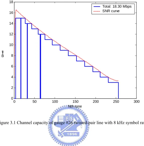
(45) C total =. N /2. N /2. ∑ b = ∑ (1 + i =1. i. i =1. SNRi ) ……………………………..……………………………..(3.3) Γ. From the previous derivation, the throughput of the DMT-based DSL system depends on the length of loop and the bandwidth used, as shown in the above equations. If the same FFT size (N=512) of the DMT system is maintained, the bandwidth of each sub-channel is proportional to its symbol rate. However, it becomes saturated after the symbol rate being increased to a certain value, as shown in reference [10]. It can also be observed from Fig. 2.7 and Fig. 2.9 that the magnitude of the channel response H(f) decreases in high frequency range especially for long loop. To observe the relationship between the channel response and its capacity, the scaled channel response magnitude in frequency domain vs. the corresponding bit-loading is shown in Fig. 3.1. We use gauge #26 twisted-pair line with 1200 m as an example, the dotted line is the magnitude of the channel response “H(f)”. The solid line as a down-stair curve represents the bit-loading of each tone, its value depends on the signal-to-noise ratio (SNR), which is the corresponding magnitude of channel response represented as the dotted line. The channel capacity can be calculated by multiplying the total bit-loading of each tone with the symbol rate. All the test loops introduced in the first chapter are simulated. In Fig. 3.1, the result of 1200 m TP1 loop is illustrated as an example. As shown in Fig. 3.1, the SNR curve cause the numbers of bits loaded in each sub-channels decrease in decent order.. 31.

(46) 18 Total: 18.30 Mbps SNR curve. 16 14 12 10 st i B. 8 6 4 2 0. 0. 50. 100. 150 Nth tone. 200. 250. 300. Figure 3.1 Channel capacity of gauge #26 twisted-pair line with 8 kHz symbol rate.. Since the magnitude of the channel response decreases at high frequency, the bits carried are lowered in those corresponding sub-cannels. Those tones with bit-loading smaller than 2 are not activated; therefore, the channel capacity has its limitation even though the symbol rate can be increased much higher. Currently, due to the increased population of fiber on the telecommunication network, the last mile of twisted-pair line can be gradually reduced to below 1.5 km, especially in the urban areas. The available frequency spectrum of these short copper wires for transmission becomes much broader and its channel capacity grows dramatically. For example, VDSL system can provide up to 52 Mbits/s over short telephone line to meet the broadband access-network requirements. It can be regarded as an evolution of the ADSL system. Several VDSL system architectures have been proposed [4][5][6][7]. These systems use the 32.

(47) frequency band from a few hundred kHz to beyond 10 MHz over some loops. In [7], we propose an asymmetric VDSL system, which is upgraded from a DMT-based ADSL system by multiplying the symbol rate. Its architecture and symbol format are the same as the original ADSL system except that both clock rate and frequency bandwidth are increased in the same ratio. Recently, the new standard for ADSL2 [13] has been announced, which also doubles the traditional ADSL bandwidth and FFT size to upgrade the throughput. No matter which method is selected, to improve the throughput of the whole system, the sampling rate should be increased to a certain ratio, which is proportional to the frequency bandwidth extension. In this chapter, the optimal channel capacity of this proposed system is analyzed over VDSL test loops at various sampling rates. This optimal channel capacity has its upper-bounded limitation due to the characteristics of the twisted-pair channel. In addition, some interference or noise types such as crosstalks and other background noises, are taken into consideration and analyzed also in this section. In this dissertation, a new factor called averaged sub-channel power spectral density (PSD) flatness is defined and calculated over VDSL test loops with various symbol rates. This factor is computed to make sure that the DMT technology can be applied at higher symbol rate if the length of twisted-pair line is shorter, such as VDSL system. Sub-channel PSD flatness factor in this dissertation is defined as the magnitude difference (in dB) of two consequent sub-channels in frequency domain. This factor indicates the variation of PSD in each sub-channel. It should be approximately flat in the region that no transmission distortion is evident, a basic assumption of DMT system. The averaged PSD sub-channel flatness is obtained by taking the average of all used sub-channel PSD flatness. In traditional ADSL system, the averaged sub-channel PSD flatness difference between adjacent sub-channels varies from 0.23 to 0.35 dB for the eight loops in T1.413. This factor depends on the length and topology of a tested loop as well as the bandwidth of a 33.

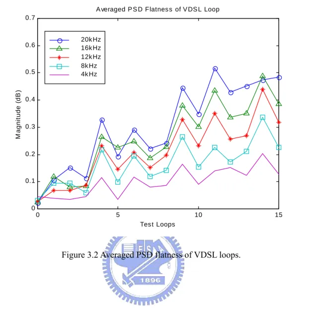
(48) sub-channel. In our proposed VDSL system, both the symbol rate and the bandwidth of each sub-channel are increased, thus the magnitude difference of two consequent sub-channels is increased also. If the difference varies too much, some of the sub-channel may not be used, and the DMT system performance degrades. The VDSL test loops set 1, as shown in Table 1.2 and Fig. 1.4, can be grouped into three types: short, medium, and long loops. The short group includes VDSL1~4 of length x equal to 300 m and VDSL5, and they are represented as test loop 1 to 5 in Fig. 3.2. The medium group includes VDSL 1~4 of length 1000 m and VDSL6, while the long one includes VDSL1~4 of length 1500 m and VDSL7, and they are represented as test loop 6 to 10, and 11 to 15 in Fig. 3.2. VDSL0 is used as a reference for the limitation of performance since its length is only 2m, very close to a null loop. The symbol rate varies from 4 kHz to 20 kHz, and so is the bandwidth of a sub-channel. The magnitudes of averaged PSD flatness vs. VDSL test loops with different symbol rate are displayed in Fig. 3.2.. 34.

(49) A veraged P S D Flatness of V DS L Loop. 0.7 20kHz 16kHz 12kHz 8kHz 4kHz. 0.6. M agnitude (dB ). 0.5. 0.4. 0.3. 0.2. 0.1. 0. 0. 5. 10 Test Loops. Figure 3.2 Averaged PSD flatness of VDSL loops.. 35. 15.

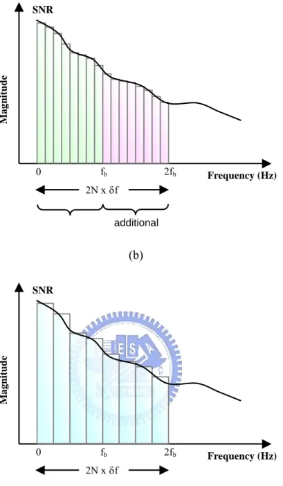
(50) 3.2 Channel Capacity vs. Symbol Rate or FFT Size In the previous discussion, one method to expand the used bandwidth is increasing the symbol rate with fixed FFT size. The other method is fixing the symbol rate but increasing the FFT size, which will increase the bandwidth at the same ratio. Therefore the total channel capacities will be close if the same bandwidth is used. Fig. 3.3 shows the relationship of FFT size and symbol rate vs. frequency bandwidth usage. Fig. 3.4 shows the simulation results of the AWGN cases with different symbol rates or FFT sizes. The dashed lines are results for FFT size extension and the solid lines are symbol rate upgrading. The variable N is the number of sub-channels for data-carrying, and the FFT size is 2N to maintain the output signal to be real instead of complex number [1][30][31].. Magnitude. SNR. unused. 0. fb. 2fb. N x δf. (a). 36. Frequency (Hz).

(51) Magnitude. SNR. 0. fb. 2fb. Frequency (Hz). 2fb. Frequency (Hz). 2N x δf additional. (b). Magnitude. SNR. 0. fb 2N x δf. Figure 3.3 FFT size and symbol rate vs. frequency bandwidth usage. (a) original (b) double FFT size (c) double symbol rate. From the simulation results, it can be seen that if the same bandwidth is used, the total throughputs of DMT- based systems are similar no matter by expanding the FFT size or by increasing the sub-channel bandwidth. For hardware based FFT implementation, if the FFT size is increased, the system complexity will increase significantly for both the FFT and IFFT blocks. 37.

(52) 140 8 kHz N=512 16 kHz N=1024 32 kHz N=2048. Bandwidth x 8. 120. 100 ) s/ st i b M ( t u p h g u or h T. 80 Bandwidth x 4. 60. 40 Bandwidth x 2 20. 0. 0. 500 1000 Test Loop Length (m). 1500. Figure 3.4 Channel capacities of VDSL system with various bandwidths (4.4, 8.8 and 17.6 MHz). For the current ADSL system, the symbol rate is only 4 kHz, and it is not difficult to increase the symbol rate by the current VLSI technology. For DSP-based FFT implementation, variable FFT block can be easily realized without additional effort only if the total computations can be completed in 232 µs [32]. Currently, the new ITU-T standard chooses the various FFT size solutions [32][33][34]. No matter which method is selected, the sampling rate should be increased by the same ratio as the bandwidth extension. For example, for the original ADSL DMT-based system with bandwidth of 1.104 MHz, the sampling rate should be 2.208 MHz to complete sampling the 512 FFT outputs plus additional 40 cyclic prefix data for a 4 kHz symbol. If the bandwidth is doubled, either by increasing the symbol rate to 8 kHz or doubling the FFT size to 1024, the sampling rate should be 4.416 MHz. The other sampling rate upgrade, such as four times or more, also expand the same bandwidth ratio. In next section, the optimal sampling rate for DMT-based 38.

(53) system under various loops and noise conditions are studied.. 3.3 Computer Simulations To verify the analysis of the relationship between channel capacity and sampling rate, some computer simulations are performed. By using the simulation results, the parameters and facts that degrade the channel capacity, such as background noise and crosstalk, are analyzed.. 3.3.1 Maximum Channel Capacity vs. Sampling Rate in AWGN Channel First, the maximum channel capacity vs. symbol rate under AWGN and system margin of various loop lengths are illustrated in Fig. 3.5 In this figure, it can also be seen that the channel capacity becomes saturated while the symbol rate is increasing to a certain value. We define the optimal sampling rate as the first point whose througput becomes more than 99% of the final maximum throughput.. 39.

(54) 250 100m 200 200m. 150 s/ st i b M. 300m 400m. 100 500m 600m 700m. 50. 0. 0. 5. 10. 15. 20 25 30 Sampling rate (MHz). 35. 40. 45. Figure 3.5 Maximum throughput of a DMT-based VDSL system under various sampling rates.. In Fig. 3.6, the theoretical maximum channel capacity vs. real system throughput with constraints are shown. The green dotted line is the theoretical value, while the blue solid lines represent the channel under system constraints. It can be seen that the degradations after considering the system constrains are in certain ratios to the ideal channel capacity. In other words, shorter loop length or higher symbol (sampling) rate results in larger loss. The optimal sampling rate also depends on the loop length. For example, if the loop length is 400 m, the sampling rate above 22 MHz would not improve the system performance much. However, for that of 700 m, the optimal sampling rate lowers to less than 11 MHz.. 40.

(55) 400 AWGN Theoretical. 350 100m 300 250 100m s/ st i b M. 200. 400m. 150. 700m 400m. 100 700m. 50 0. 0. 5. 10. 15. 20 25 30 Sampling rate (MHz). 35. 40. 45. Figure 3.6 Performance comparison of AWGN with system margin to theoretical one.. The optimal sampling rate here is defined as the frequency at which the curve is turning to the saturation state. It can be seen that before the saturation state occurs, the channel capacity increases with the sampling rate linearly. In current DMT-based ADSL system, the sampling rate is 2.208 MHz only. If it is raised to 11.04 MHz, the channel capacity can be increased from 15 Mbits/s to nearly 50 Mbits/s at loop length of 700 m. If the loop length becomes shorter, the improvement is even higher. The curves of the simulation results are lower than those in reference [1] since the SNR gap, which depends on some system parameters, such as bit error rate, coding gain, and system margin, is considered. However, the trend is the same that the channel capacity becomes saturated at high frequency, as shown in Fig. 3.6.. 41.

(56) 3.3.2 AWGN vs. VDSL Noise In VDSL standard, two types of color noise mask are included[4]. These two noise masks located at certain frequency part (below 1.1 MHz), therefore, the maximum throughput is smaller than the AWGN case with a system margin of certain amount. The simulation results for noise type A and type B are shown in Fig. 3.7 and 3.8, respectively. It can be observed that the degradation increases with the loop length. The reason is that the channel response magnitude of a longer loop is smaller but the noise density is the same, and therefore the degradation ratio increases.. 250 AWGN AGNA 100m. 200. 150 s/ st i b M. 400m 100. 50. 0. 700m. 0. 5. 10. 15. 20 25 30 Sampling rate (MHz). 35. 40. Figure 3.7 Performance comparison of noise type A with AWGN.. 42. 45.

(57) 250 AWGN AGNB 100m. 200. 150 s/ st i b M. 100. 400m. 50 700m. 0. 0. 5. 10. 15. 20 25 30 Sampling rate (MHz). 35. 40. 45. Figure 3.8 Performance comparison of noise type B with AWGN.. 3.3.3 AWGN vs. Various Crosstalk In this subsection, different crosstalk noise are simulated, such as HDSL and ADSL NEXT and VDSL FEXT, etc[35]. In general, NEXT noise is much larger than FEXT, therefore, only the NEXT of other DSL system will be dominant. Fig. 3.8 shows the HDSL NEXT case, the degradation is less than 5% because its bandwidth of power spectrum is concentrated below 400 kHz. For the 512-FFT and symbol rate of 10 kHz VDSL system, its bandwidth is 5 MHz. Therefore, its effect is not so significant. The second one is the ADSL downstream NEXT case, its power spectrum bandwidth is up to 2.2 MHz and has more effect on the system performance, as shown in Fig. 3.10.. 43.

(58) 250 AWGN HDSL-NEXT 100m 200. 150 s/ st i b M. 400m. 100. 50. 0. 700m. 0. 5. 10. 15. 20 25 30 Sampling rate (MHz). 35. 40. 45. Figure 3.9 Performance comparison of HDSL NEXT crosstalk with AWGN. 250 AWGN ADSL-DS-NEXT 100m 200. 150 s/ st i b M. 400m. 100. 50 700m. 0. 0. 5. 10. 15. 20 25 30 Sampling rate (MHz). 35. 40. 45. Figure 3.10 Performance comparison of ADSL NEXT crosstalk with AWGN.. 44.

(59) 250 AWGN VDSL-FEXT 200. 100m 150 s/ st i b M. 100. 400m. 50. 700m. 0. 0. 5. 10. 15. 20 25 30 Sampling rate (MHz). 35. 40. 45. Figure 3.11 Performance comparison of VDSL FEXT crosstalk with AWGN.. In DMT-based VDSL system, if the synchronous system is used, the NEXT problem can be discarded. Therefore, only the FEXT should be considered. It is clear that this FEXT depends on the loop length. The shorter the loop is, the larger the degradation will be, as shown in Fig. 3.11. This result is reasonable because the crosstalk coupling from the far end will decay more through the long loop length.. 3.3.4 AWGN vs. Bridged-taps In general, the bridged-taps can cause notches for VDSL length loops. If some bridged-taps of various lengths are added into the middle of a tested loop, the shortest bridged tap causes the deepest null [1][5]. In our test case, we use the bridged-tap type as shown in [3], and the simulation results are shown in Fig. 3.12.. 45.