氫原子在不同偏振光的Pump和Probe雷射照射下之效應

國立交通大學

物理研究所

碩士論文

氫原子在不同偏振光的 Pump 和 Probe 雷射照射下之效應

Polarization Effect of Pump-Probe Process on Hydrogen Atom

研 究 生：吳明軒

指導教授：江進福 教授

氫原子在不同偏振光的Pump和Probe雷射照射下之效應

研 究 生：吳明軒

Student：Ming-Hsuan Wu

指導教授：江進福

Advisor：Tsin-Fu Jiang

國立交通大學

物理研究所

碩士論文

A Thesis Submitted to Institute of Physics College of Science National Chiao Tung University in partial Fulfillment of the

Requirements for the Degree of Master in

Physics June 2010

Hsinchu, Taiwan, Republic of China

中華民國九十九年七月

氫原子在不同偏振光的 Pump 和 Probe 雷射照射下之效應

學生：吳明軒 指導教授：江進福

國立交通大學物理研究所碩士班

摘要

氫原子在雷射 pump 和 probe 照射下，利用由

N. N. Choi 和 T. F. Jiang 等

人所建立的 pump-probe 模型，計算當氫原子在 pump 雷射照射後，接著照

射一 probe 雷射來獲取干涉過程之資訊。並改變 probe 雷射之方向，計算

其不同偏振下的效應。

Polarization Effect of Pump-Probe Process on Hydrogen Atom

Student：Ming-Hsuan

Wu Advisor：Dr. Tsin-Fu Jiang

Institute of Physics

National Chiao Tung University

ABSTRACT

In pump-probe process, the probe laser was applied to retrieve the

information of electron’s dynamics on atoms or molecules after the pump laser

process finished. In this thesis, we used the pump-probe model constructed by N.

N. Choi and T. F. Jiang et al., to investigate the interference effect on the

hydrogen atom. Besides, we used linear and elliptical polarization on probe laser

to study how polarization effect affected on the hydrogen atom in pump-probe

process.

誌謝

感謝指導教授江老師耐心得指導，每次的 meenting、課程上以及討論

都讓我獲益良多，激發很多在論文上的想法以及學習研究的方法，也讓我

明瞭理論模型在物理學上的重要性。也非常感謝博士後研究員的李漢傑博

士和鄭世達學長，在我對理論知識不足的情況下，總是犧牲自己的研究時

間耐心地教導我、替我尋找有用的資料，補足我對論文題目的了解。在我

對 LINUX 作業系統以撰寫程式上有迷惑時，感謝李允民博士和鄭玉書同學

的幫忙和協助。也感謝曾給予建議協助的師長們，以及在夜晚寂靜地研究

室陪伴我敲打電腦的學長張繼允和奈米所學弟謝孟哲，還有在剛踏入交大

校園裡帶我認識物理所的徐煥鈞學長，感謝。

在研究的過程中，支持著每一步往前進的動力，除了對物理感到好奇的

這份拉力，家人總是在身後默默給予支持。感謝老媽、老樺、大哥和女友

的照顧、支持、電話的問候和寫作論文上的幫助，你們是我前進的主要動

力，也是我這一生最重要的人，我愛你們。

要感謝的人還很多，在新竹的大學同學，以前大學教授和大學室友等

等，但唯一最好的回報，就是不會辜負你們對我的期望，繼續努力。

目錄

中文提要…...………... …...………...……Ⅰ 英文提要…...………... …...………...…Ⅱ 誌謝…...………... …...………...Ⅲ 目錄…...………... …...………...Ⅳ 符號說明…...………... …...………...…Ⅴ 圖目錄…...………... …...………...……Ⅵ Chap 1. Introduction………...……...1

Chap 2. Pump-probe model…...………...4

Chap 3. Considering one excited states in pump probe model………...…...7

3.1 Two-level system..………...………...………10

3.2 1st order time dependent perturbation theory………...….…...15

3.3 Numerical result.………...22

Chap 4. Considering two excited states in pump probe model…...…...24

4.1 Three-level system.………...………...….…..27

4.2 Numerical result…….………..……..31

Chap 5. Linear and elliptical polarization effect.……….……….…….34

5.1 Linear polarization.………...……….34

5.2 Ellipitical polarization...………...………...49

Chap 6. Conclusion……….……….………..60

Reference……….……….61

符號說明

2

|

|Mif

：The angle-resolved photoelectron probability density

t

d

：The time delay

ε

k

：Photoelectron energy

,

k k

θ ϕ

：The polar and azimuth angle of photoelectron emissive direction

,

l l

θ ϕ

：The polar and azimuth angle of Probe laser pulse’s direction under

dipole approximation

P

：The total probability of photoelectron ionization

k

dP

d

ε

：The energy-resolved photoelectron probability density

List of Figure

1.1 The SAP and APT in time and energy domain……….………..2

1.2 The typical high-harmonics spectrum……….……….………...2

2.1 The APT and IR pulse in time domain in pump-probe process………..4

3.1 The mechanics for considering one excited state in pump-probe model………7

3.2 Two-level system……….……….………....10

3.3 Comparing the numerical result of RK4 method to analytical solution…………...12

3.4 Comparing the numerical result of RK4 method to exact solution………...13

3.5 The population of two-level system………..14

3.6 Checking the continuum state of CPC’s program with asymptotic form………….16

3,7 Photoelectron energy spectrum _{| |}2 if M for considering one excited state…….…22

3.8 The _{| |}2 if M depends on εk and td for considering one excited………23

4.1 The mechanics for considering two excited states in pump-probe model…………24

4.2 Three-level system……….……….………27

4.3 Comparing the numerical result to the exact solution…. ……….……….29

4.4 The population of three-level system……….………...30

4.5 Photoelectron energy spectrum _{| |}2 if M for considering two excited states……...31

4.6 The energy-resolved probability density depends on time delay ………...32

4.7 The total probability depends on td……….………..32

4.8 _{| |}2

if

M depends on εk and td for considering two excited states in pump-probe model……….……….……….……..33

5.1 _{| |}2

if

M depends on εk and td for differentθl……….………..36

5.2 3D diagram of _{| |}2

if

M depends on θ_k and ϕ_k for linear polarization………37

5.3 The _{| |}2

if

M depends on θ_k for linear polarization……….………..39

5.4 3D diagram of _{| |}2

if

M depends on different θ_l….. ……….………40

5.5 The interference part of Eqs. (5.3)……….………42

5.6 The diagram for the asymmetry parameter……….……….……….43

5.7 The _{| |}2

if

M and asymmetry parameter depends on td ……….44

5.8 The _{| |}2

if

M depends on depends on θ_k for different CEP ………..…45

5.9 Reconstruct the _{| |}2

if

M dependent on θ_k for linear polarization…….…………47

5.10 The probability of ionization depends on θl……….………48

5.11 The _{| |}2

if

5.12 The _{| |}2

if

M depends on θ_k for circular polarization…. ……….……….51

5.13 3D diagram of _{| |}2

if

M depends on θ_k and ϕ_k for α=1………....52

5.14 3D diagram of _{| |}2

if

M depends on θ_k and ϕ_k for α=2………53

5.15 3D diagram of _{| |}2

if

M depends on θ_k and ϕ_k for different α………..54

5.16 The interference part of Eqs. (5.15)………..55

5.17 The _{| |}2

if

M depends on θ_k for different α………...56

5.18 The total probability of ionization depends on α………..…56

5.19 The _{| |}2

if

M depends on px and pz for different θ_l……….…..58

5.20 The _{| |}2

if

Chapter 1

Introduction

In recent years, the attosecond science is very popular to measure the electron dynamics on its nature time scale, the time of that an electron make a cycle on atom, which is about 24 attoseconds. In pump-probe experiements, try to apply a pump laser with time delay between the probe laser which interfering on the wave packets with the pump laser and has the goal to unravel the dynamics of atoms or molecules. Such experiments have the advantage that the time delay can be controlled with high precision at the level of attoseconds. There are two type of attosecond pulse can be produced in the laboratory. One is the single attosecond pulse (SAP), wider spread in frequency for short pulse duration, and the other one is attosecond pulse trains (APT) , which in the extreme ultraviolet can be produced in the process of high-order harmonic generation (HHG) by exposing rare gas atoms to intense femtosecond infrared (IR) laser pulses. To see the difference between SAP and APT in time and energy domain in Fig. 1.1. The width spread in frequency can be calculated by Δω=4ln2/Δτ, where the Δω is the pulse’s full width of half maximum (FWHM) in frequency domain and the Δτ stands for the pulse duration of FWHM, so the Δω ≈1.83/Δτ , Δτ in fs unit. Thus today only a handful of laboratories are capable of performing APT+IR or SAP+IR experiments, where the IR is the femtosecond infrared (IR) laser pulses. N. N. Choi and the T. F. Jiang, etc. construct a simple theory[1], a pump-probe model , analytically and successfully to explane the pump-probe experiments. Here , we use the APT+IR process as they do.

The APT are synthesized from the high harmonics generated by HHG in plateau region, as showed in Fig. 1.2

The form of APT pulse can be written down as

odd

n

t

n

E

t

E

n n

=

+

=

∑

= =

),

sin(

)

(

29 11 0

ω

ϕ

(1.1)

Figure. 1.1 The SAP and APT in (a) time domain and (b) energy domain. The width of FWHM for blue, green and red pulse is 6ev, 0.9ev, and 0.183 ev. (P. Ranitovic et al., 2010[2])

(a) (b)

where the E is the APT pulse envelope, and the the carrier envelope phase (CEP) ₀ ϕ is fixed.

In this thesis, we simulate the APT pulse on the hydrogen atom to dissus the pump-probe process, and then briefly introduce the pump-probe model by the T. F. Jiang, etc. in chapter 2. In chapter 3, we introduce only considering one excited state system, Ψ on hydrogen ₂₁₀ atom, and show the numerical result. Futermore, In chapter 4 consider two excited states,

310

Ψ and Ψ , in the pump-probe model which totally three wave packets interfere with ₄₁₀ each other, and then show the numerical result. In chapter 5, consider the linear polarization effect by aligning the probe laser to different direction between pump laser to retrieve the information in pump-probe process. Finall, the last chapter, chapter 6, is the conclusions about this thesis.

chapter 2.

Pump-probe model

In pump probe model, there are two pulse laser, pump and probe laser, applied to the target, and here we use hydrogen as the target. The first laser coming into the system called first path for the interference uses APT (Attosecond Pulse Trains) pulse as pump laser, and then the second laser called second path for the interference uses IR pulse to be the probe laser. APT pulse can drive the electron of the hydrogen to jump probably to continuum state and excited state, if the APT pulse’s for some high-harmonics frequency (to see Eqs. (1.1) )are nearly resonant for some excited states. Then, a time delay after the APT pulse ending, the IR pulse comes into the system and has weaker energy then APT pulse to contribute the probability for the electron from the excited state to the continuum state. Finally, the two paths will interfere with each other in the energy spectrum.

In the beginning of pump-probe process, define t=0 to be at the center of the APT pulse. The time difference between the APT pulse’s center and IR pulse’s center is defined as the time delay τ. For clarity, the Hamiltonian of such a dynamic system can be written in the

Figure. (2.1) The diagram for pump APT pulse and probe IR pulse in time domain in pump-probe process.

dipole approximation as

)

(

ˆ

)

(

0

+

+

ε

⋅

−

τ

=

H

zE

t

r

E

t

H

_x

r

_L (2.1)

where, the APT pulse is aligned to parallel with z axis, and for being interested in the effect about the different laser direction between APT pulse and the IR pulse, we applied the IR pulse direction at εr⋅rˆ.

To consider only the situation in that the pump and probe laser do not overlap, so we can write down the total evolution operator (propagator) for the pump and probe laser as

)

2

,

2

(

)

2

,

2

(

0 x x x t iH L L L total

U

e

U

U

=

τ

+

τ

τ

−

τ

⋅

− d

⋅

τ

−

τ

(2.2) where, the td is defined to the time different between the APT pulse ending and the IR pulse starting, and the _e−iH0td is the propagator of Hamiltonian under no any external field.

Represent the atomic evolution operator _e−iH0td in terms of the excited (bounded state) and

continuum eigenstate , |n>, and eigenenergy En of H0

∑

>

<

=

− − n t iE t iH

n

e

n

e

0d

|

nd

|

(2.3) Therefore, the total evolution operator Utotal can be rewriten to

)

2

,

2

(

|

|

)

2

,

2

(

x x x t iE L L L n total

U

n

e

n

U

U

=

∑

τ

+

τ

τ

−

τ

⋅

>

− nd

<

⋅

τ

−

τ

(2.4) Write down the transition probability amplitude as a function of time-delay for transit from initial bound state |i> to an final ionized state | f >

>

−

<

⋅

⋅

>

−

+

<

=

>=

=<

− →

∑

f

U

n

e

n

U

i

M

i

U

f

M

x x x t iE L L L n if total f i d n

)

|

2

,

2

(

|

|

)

2

,

2

(

|

|

|

τ

τ

τ

τ

τ

τ

(2.5)

paths represented by the intermediate state |n>, and the transition amplitude is contributed from the intermediate state |n> to the final ionized state | f >. The APT pulse can pump the electron probably to some excited states of hydrogen atom and ionized state, so we choose the intermediate state as bounded state and unbounded state. In chapter 3, we consider continuum state and only one bounded state to be intermediate states. In chapter 4, we add one more bounded state, two bounded states, and continuum state to be intermediate states.

Chapter 3.

Considering one excited state in pump-probe model

For considering one excited state in pump-probe model, we choose first excited state of hydrogen atom |2p> as bounded state, and another one is continuum state |k′> as unbounded state. The electron in ground state is ionized by the first laser, APT pulse that we simulating only two high-harmonic orders frequency, one makes the probability to excite to the unbounded state, the second one to ionize to continuum state | k′> , and finally is driven to the other continuum state |k > by the second laser, IR pulse. There are two paths interfering with each other at same energy spectrum. To describe the dynamics system, as showed in Fig. 3.1. 2p 1s ω ω1 2p Continuum state Eenergy [ev] -13.6 -3.4 ω2 10.2 ev pump (APT) probe (IR)

+

→

Figure. 3.1 The mechanics for considering one excited state in pump-probe model. The ω1 = 10.1 ev, ω2 = 15.1 ev, ω= 5 ev

In the Fig. 3.1, the beginning of the electron in initial ground state |1s> is probably ionized by the APT pulse to the first excited state |2p> and continuum state |k′>, and then driven to the continuum state |k > by the IR pulse in weak frequency to the same energy spectrum. We let the initial, intermediate and final state as

>

′

>

>=

>

>=

>

>=

k

and

p

n

k

f

s

i

|

2

|

|

|

|

1

|

|

(3.1)

here (and throughout the thesis) |k > dose not denote a plane wave but a scattering wave which is an eigenstate of H0 with incoming boundary conditions. Therefore, for considering one excited state in pump-probe model, we can write down the transition probability amplitude as

∑

′ ′ ′ − − _′

+

=

k s k k k t i s p p k t iE if

e

M

M

e

M

M

M

pd k d 1 , , 1 , 2 2 , 2 ε (3.2) where the M_2p,1s, and M_k,′1s are probability amplitudes for transition induced by the APT pulse, and the M_k,2pand M_k,k′ are the probability amplitudes for transition induced by the probe IR laser pulse, and the E2p and εk are the eigenenergy of H0 for |2p> state and the

> ′ k

| state.

For the intermediate state |k′> transition to the continuum state |k >, the free electron does not change the momentum and the energy by the IR laser pulse but accumulates the phase which is called Volkov phase during the free electron propagating time. To use the Volkov phase approximation

∫

− ′

=

−

′

−

2

+

2 2 ,

(

(

))

]

2

exp[

)

(

L L

k

A

t

dt

i

k

k

M

_kk τ τ

δ

r

r

_(3.3)

where Ar(t) is the vector potential of the probe IR laser pulse. Finally, the transition

s k k i t i s p p k t iE if

e

M

M

e

e

M

M

pd k d L k 1 , ) ( 1 , 2 2 , 2 −ε − τ ⋅ε +α⋅ +β − _′

+

=

rr (3.4) where

∫

−+

−

=

2 2

)

(

L L

A

t

dt

τ τ τ τ

τ

α

r

r

_and

_∫

+ −

−

=

2 2 2

₍

₎

L L

A

t

dt

τ τ τ τ

τ

β

_(3.5)

To change the variables, we can find the α and β are independent on the time delay τ.

∫

−

=

2 2

)

(

L L

A

t

dt

τ τ

α

r

r

_and

_∫

−

=

2 2 2

₍

₎

L L

A

t

dt

τ τ

β

_(3.6)

For clarity to see the magnitude and phase in the transition probability amplitude, we define that

)

exp(

1

|

|

)

exp(

1

|

|

2

)

exp(

2

|

|

, , 1 , , , 1 , 2 , , 2 , s k s k x s k s p s p x s p p k p k L p k

i

a

s

U

k

M

i

a

s

U

p

M

i

b

p

U

k

M

ϕ

ϕ

φ

⋅

>=

=<

⋅

>=

=<

⋅

>=

=<

(3.7)

Finally, the ionization probability density is expressed as

[

]

)

(

)

(

)

(

cos

|

)

(

|

, , , 2 , , , , 2 , 2 , 2 2 p k s p L k s k d p k s p p k s k s p p k s k d if

k

t

E

a

b

a

a

b

a

t

M

φ

ϕ

β

α

τ

ε

ϕ

ε

+

−

+

⋅

+

−

=

Φ

−

−

Φ

+

+

=

r

r

(3.8)

Eqs. (3.8) gives some information about the mechanism in pump-probe model. The first term gives the probability for producing an electron with momentum k by APT pulse. The second term is the probability for the electron exciting to the |2p>state by the APT, and then ionizing to the same continuum state |k > with same final momentum k. The last term is due to the interference of the two different paths, where the time delay dependence is explicitly expressed clearly. The phase in cosinusoidal function including the phase of the excitation and ionization amplitude is contributed by the pump APT pulse and probe IR pulse, and dose not depend on the time delay td.

3.1 Two-level system

Consider the interaction of a radiation electric field E(t) of energy ω with a two-level hydrogen atom system, |1s>and |2p > .Let |1s> and |2p> represent the hydrogen ground state (the lower level) , and excited state with quantum number n=2 and l=1 (the upper level). we can describe the total wave functionin the formof

>

+

>

>=

Ψ

(

t

)

C

_s

(

t

)

|

1

s

C

_p

(

t

)

|

2

p

|

_{1 2} (3.9)

where )C_1s(t and C_2p(t) are the probability amplitudes of finding the electron in states >

s 1

| and. |2p>In the interaction picture, we can let the time-dependent coefficient

t iw s s a e t c t

C₁ ( )= ₁ ( ) − , and the Schro&&dinger equation can chage to

>

+

>

>=

Ψ

− −

p

e

t

c

s

t

e

t

c

t

)

_s

(

)

i st

(

)

|

1

_p

(

)

i pt

|

2

(

|

1 2 2 1 ω ω h h (3.10) where hω1s and hω2p are the eigenenergy of |1s>( ≈ -13.6 ev) and |2p>( ≈ -10.2 ev).

The corresponding Hamiltonian of the Schro&&dinger equation is

H

H

H

=

₀

+

′

(3.11)

where the unperturbed part Hamiltonian H is ₀

|

2

2

|

|

1

1

|

₂ 1 0

s

s

p

p

H

=

_h

ω

_s

><

+

_h

ω

_p

><

(3.12) Figure 3.2. △ω=10.2 ev, ω=10.1 ev

and the perturbed part H ′ is

)

cos(

]

)

(

2

ln

2

exp[

ˆ

ˆ

)

(

2 X X m

t

t

E

z

z

t

E

H

′

=

⋅

=

⋅

⋅

−

_τ

⋅

ω

+

φ

(3.13)

The unperturbed part H ′ Eqs. (3.13) ,where Em is the maximum amplitude of electric field E(t), and τX is the duration time of E(t), and φX is the carrier envelope phase (CEP) of the pump APT pulse E(t).

The equation of motion for the amplitude coefficient c₁s(t) and c2p(t) may be written

as 1 2 2 1

( )

1 | | 2

( )

2

( )

2 | |1

( )

2

i t m s p i t m p s

E

ic

t

e

s z

p

c

t

E

ic

t

e

p z

s

c

t

− Δ Δ

=

⋅

<

>

=

⋅

<

>

&

&

(3.14)

In deriving the Eqs. (3.14), we have ignored the emission photon term, and only considered the absorbtion photon term propotional to exp[±i(ω−(Δω)] on the right hand side in rotating wave approximation (RWA). Here, we use the 4th _{order Runge Kutta method (RK4)} to solve the Eqs. (3.14).

Fianlly, we want to check my program, so use two special cases to check my program code. First, the case one is frequency of electric field equals resonant frequency ω. We derive the analytical solutions for the special calse when ω equals the resonance frequency Δω. Let the coefficient to i r p i r s

ib

b

c

ia

a

c

+

=

+

=

2 1 (3.15)

"

"

0

"

"

0

)]}

(

1

[

2

sin{

)

(

)]}

(

1

[

2

cos{

)

(

−

>

−

≥

+

>

−

≤

Ω

=

Ω

=

t

t

t

a

erf

a

t

b

t

a

erf

a

t

a

i r

τ

τ

π

τ

τ

π

m

m

(3.16)

To use Eqs. (3.16) to compare my numerical result of RK4 method

Secondly, the case two is for the electric field being no pulse’s shape, likeE(t)=Emcos(ωt) and the solution is (see [3] )

{

[

]

}

{

[

]

}

⎪ ⎪ ⎩ ⎪⎪ ⎨ ⎧ Ω Ω Ω + Ω Ω Δ + Ω = Ω Ω Ω + Ω Ω Δ − Ω = ⇒ Δ − Δ 2 / 1 2 2 2 / 2 1 1 ) 2 sin( ) 0 ( ) 2 sin( ) 2 cos( ) 0 ( ) ( ) 2 sin( ) 0 ( ) 2 sin( ) 2 cos( ) 0 ( ) ( t i s R p p t i p R s s e t C i t i t C t C e t C i t i t C t C (3.17)

Figure. 3.3 The lines is by the RK4 method, and the points (+) are by the analytical solution. Em=0.1 (a.u.), FWHM = 5 (fs). The result of RK4 well fits in with the analytical solution.

Figure. 3.4 Em=0.1 (a.u.), Δ=ω21×95%. The upper figure is population of 2-level system and the line (−) is by the analytical solution, and points (×) are by the RK4 method. The lower figure is the error of the amplitude in 2-level system. The thin line is errors for the amplitude of real part, and the thick line is of imagine part.

Finally, the probability for |1s> excitating to |2p> calculated by numerically is about 17.82%.

Figure. 3.5 The thin line is the population of the |1s> state, and the other one is of the |2p> state. Finally, the probability of finding the electron at

> p 2

| is about 17.82% . The peak intensity and FWHM of pump APT pulse laser is respectively 2.3×1013 _W/cm2 _{and 8.5 fs.}

3.2 1

st

order time dependent perturbation theory

When the applied electric field is not very strong, we can calculate the ionization probability by using the 1st time dependent perturbation theory. The amplitude by 1st time dependent perturbation theory is

( ) 0

( )

k n

|

|

t _i n k

i

C

_→r

t

= −

∫

e

ε ε−

⋅ <

k H

r

′

n

>

dt

h

)

(

)

(

)

(

|

( ) 0 r lm k lm l i l l l l m

Y

Y

r

kr

F

e

i

k

>=

− l

⋅

⋅

∗

Ω

Ω

= =−

∑ ∑

σ

r

(3.18) where |k > is the continuum (unbounded) state with eigenenergy εk and momentum k, the

> n

| is the bounded state with eigenenergy En, the Ω is the angle for photoelectron and the k l

σ is the phase shift due to coulomb potential. In the pump probe model, we use the 1st time dependent perturbation theory to calculate the probability density for electron ionizing respectively from |1s > and |2p> to the unbounded state |k >.

Here, we use the CPC’s (computer physics communication) program [4] to construct the continuum wave equation Fl(kr). For checking the continuum wave equation, try to compare the continuum wave equation to the electron asymptotic wave equation at far distance between the neutron

) 2 ln 2 sin( 2 1 ) ( l kr l kr l kr k r r kr F π _{γ σ} π − − + ⎯ ⎯ → ⎯ →∞ _(3.19) where k 1 − =

γ for hydrogen atom. Fig. 3.6 is the result for the continuum wave function of CPC’s program comparing to asymptotic form.

Figure. 3.6 The upper figure is about radius from 0 to 30 (a.u.) at photon energy εk= 0.05 (a.u.). The errors of the lower figure is bigger then upper one at the short distance between the neutron, but when the radial distance is enough to neglect Coulomb potential of hydrogen atom, the continuum wave function |k > can be well identify with asymptotic wave function together.

There is still one thing that we should care about the Eqs. (3.18) starting at t = 0. In pump probe model , the pump pulse comes into the system at t = −τX /2, so we have to modify the amplitude of 1st _{time dependent perturbation. To redrive the Eqs. (3.18) will contribute the}

phase shift about ( ) 2

X n k i

e

τ ε ε − ⋅

, as showed in Eqs. (3.23). The wave function is the superposition of eigenstate | n>

∑

>

>=

Ψ

− + n t i n

t

e

n

C

t

x n

|

)

(

)

(

|

( 2) τ ε (3.20)

and the time dependent

Schr

o

&&

dinger

equation is

]

|

|

)

(

[

]

|

)

(

)

(

|

)

(

[

)

(

|

]

ˆ

[

)

(

|

) 2 ( ) 2 ( ) 2 ( ) 2 ( 0

>

′

+

>

=

>

−

+

>

⇒

>

Ψ

′

+

>=

Ψ

+ − + − + − + −

∑

∑

n

H

e

n

e

t

C

n

e

t

C

i

n

e

dt

t

dC

i

t

H

H

t

dt

d

i

n t i n t i n n t i n n n t i n x n x n x n x n

ε

ε

ε

τ ε τ ε τ ε τ ε

h

h

(3.21)

Expand

C

_n

(t

)

in perturbation series

L

+

+

=

(

)

(

)

)

(

t

C

(0)

t

C

(1)

t

C

n n n (3.22)

To intergrate the above Eqs. (3.21) will contribute a phase shift to probability amplitude

∫

∫

− ′ − − − + ′ − →

′

>

′

<

−

=

′

>

′

<

−

=

t T t i i t T t i k n

t

d

n

H

k

e

e

i

t

d

n

H

k

e

i

t

C

n k x n k x n k 2 ) )( ( ) 2 )( ( 2 ) 2 )( ( ) 1 (

|

|

|

|

)

(

ε ε τ ε ε τ ε ε

h

h

(3.23)

2 ) ( x n k i

e

τ ε ε − ⋅

. The form of APT pulse for some high-harmonic order frequency which can ionizes the electron to continuum state is

2

ˆ

ˆ

( )

exp[ 2ln 2(

) ] cos(

)

pump m X x

t

H

′

=

E t

⋅ = ⋅

z

z E

⋅

−

_τ

⋅

ω φ

t

+

(3.24)

In pump probe model, we have to calculate C(1)1s→k(t) and C(1)2p→k(t). For the hydrogen

atom , the ground state |1s > is

⎭

⎬

⎫

⎩

⎨

⎧

⎭

⎬

⎫

⎩

⎨

⎧

=

>=

−

π

4

1

2

)

1

(

1

|

0 / 2 / 3 0 00 10 a r

e

a

Y

R

s

(3.25)

Here we use the atomic unit, so the |1s> is

{ }

⎭

⎬

⎫

⎩

⎨

⎧

>=

−

π

4

1

2

1

|

r

e

s

_(3.26)

The transition amplitude from |1s > to |k >

1 2 1 1 2 ( )( ) _{( )( )} (1) ₂ 1 2 2 ( )( ) _{( )( ) 2ln 2( )} 2 2 2 ( )( ) 1 2

( )

|

|1

2

| |1

cos(

)

[

(

)]

1

| |1

2

4

k n k s k s k n k s x x x i _{i t} x s k pump x x x t i i t _x m x x x i _i k s m

C

ie

e

k H

s

dt

ie

E

k z

s

e

e

t

dt

E

ie

E

k z

s

e

e

a

a

τ τ ε ε _{ε ε} τ τ τ ε ε _{ε ε} τ τ τ ε ε _ϕ

τ

ω φ

ω ε

π

− _{− ′} → − − _{− ′ −} − − ₋

′

′

= −

<

>

′

= −

⋅ <

>

⋅

+

⎧

_{− −}

₋

= −

⋅ <

>

∫

∫

⎫

⎪

⎪

⎨

⎬

⎪

⎪

⎩

⎭

(3.27) where the <k|z|1s> is the dipole matrix element which can be calculated by the numerical method, a is 2ln2 ₂

X

τ for the electric Gaussian pulse, and here we fix the φX =0. The

∫

∑

_∫

_∫

∗ ∗ ∗

⋅

Ω

−

=

⋅

⋅

Ω

⋅

⋅

Ω

−

=

>

>=<

<

10 2 10 , 00 10 3

)

(

)

(

3

)

(

cos

)

(

)

(

)

(

1

|

cos

|

1

|

|

1

_Y

_dr

_r

_F

_kr

_R

e

i

Y

Y

d

R

r

kr

F

r

dr

Y

e

i

s

r

k

s

z

k

l k i m l lm r l k lm i l _l σ σ

_θ

θ

(3.28)

so the transition amplitude finally becomes

) ( ) exp( ₁₀ 1 ) 1 ( k x x k s A i Y C → = ϕ ⋅ Ω (3.29) where X s k x l s k m x x E R kr F r dr a a E e E A φ σ τ ε ϕ π ε ω − + − = ⋅ ⎭ ⎬ ⎫ ⎩ ⎨ ⎧ − − − ⋅ − =

∫

∗ 1 1 10 2 2 1 ) 2 )( ( ) ) ( ( 4 )] ( [ 3 1 (3.30)

For the second path from |2p> to |k >, the probe IR laser pulse is used to

[

]

2 0

ˆ

ˆ

ˆ

ˆ

( )

exp[ 2 ln 2(

) ] cos

(

)

probe L L

t

H

′

=

E t

ε

⋅ = ⋅ ⋅

r

ε

r E

⋅

−

−

τ

_τ

⋅

ω

t

− +

τ

ϕ

where the E is the maximum amplitude, ₀

ε

ˆ

⋅

rˆ

is the direction,

τ

L is the duration time

and the CEP of IR lasse pulse

ϕ

L= -π/2. Secondly, to calculate the transition amplitude from

> p 2 | state to the |k > 2 2 2 ( )( ) _{( )( )} (1) ₂ 2 2 2 ( )( ) ₂ 2 0

( )

|

| 2

2

[

(

)]

1

ˆ ˆ

|

| 2

2

4

L L k n k p L L k p L i _{i t} L p k probe i _{k p} i

C

ie

e

k H

p

dt

E

ie

E

k

r

p

e

e

a

a

τ τ ε ε _{ε ε} τ τ ε ε _ϕ

τ

ω ε

_π

ε

− _{− ′} → − − ₋

′

′

= −

<

>

⎧

− −

−

⎫

⎪

⎪

= −

⋅ <

⋅

_{> ⎨}

_⎬

′

′

⎪

⎪

⎩

⎭

∫

(3.31)

Here, to control the probe IR laser pulse’s direction, we expand the ε) ⋅rr to

{

[

]

}

)

,

(

)

,

(

)

,

(

)

,

(

)

,

(

)

,

(

3

4

ˆ

1 , 1 1 , 1 0 , 1 0 , 1 1 , 1 1 , 1

ϕ

θ

ϕ

θ

ϕ

θ

ϕ

θ

ϕ

θ

ϕ

θ

π

ε

Y

Y

Y

Y

Y

Y

r

r

l l l l l l ∗ ∗ − − ∗

+

+

=

⋅ r

(3.32)

where the θl is the polar angle and ϕl azimuth angle of the direction of probe laser.

Futnermore, the radial part in the Eqs. (3.31) becomes

∫

∫

∫

∫

∗ ∗ ∗ ∗ − ⋅ Ω ⋅ ⋅ − ⋅ Ω ⋅ ⋅ + ⋅ Ω ⋅ ⋅ − ⋅ Ω > ⋅ < ⋅ ⋅ − >= ⋅ < 21 0 2 0 , 0 21 2 2 1 , 2 21 2 2 0 , 2 21 2 2 1 , 2 21 2 ) ( ) ( ) sin( 3 1 ) ( ) ( ) cos( 10 1 ) ( ) ( ) cos( 15 4 ) ( ) ( ) sin( 10 1 2 | ˆ ˆ | 0 2 2 2 R kr F r dr Y e R kr F r dr Y e R kr F r dr Y e R kr F r dr Y R F e p r k k i l k i l k i l k i l σ σ σ σ θ θ θ θ ε (3.33)

Here we fix the ϕl = 0. Finally, deduce the transition amplitude for the second path to

{

}

{

}

) ( cos 4 3 ) ( ) ( ) ( ) ( ) ( ) ( ) , ( 0 , 1 0 , 0 3 0 , 2 2 1 , 2 1 , 1 1 , 2 1 , 1 1 2 1 1 k i l k i k i k l k l i l l if Y be Y e a Y e a Y Y Y Y e a M b Ω + Ω + Ω + Ω Ω + Ω Ω = ∗ − − ∗ ϕ ϕ ϕ ϕ θ π ϕ θ (3.34) where

{

}

{

}

{

}

{

E

}

r F R dr E b dr R F r M E E a dr R F r M E E a dr R F r M E E a x x s k pump m s p L L p k probe s p L L p k probe s p L L p k probe 10 1 2 2 2 2 1 21 0 2 1 , 2 2 2 2 2 0 3 21 2 2 1 , 2 2 2 2 2 0 2 21 2 2 1 , 2 2 2 2 2 0 1 2 ln 2 2 ln 8 )] ( [ exp 2 3 2 | | 2 ln 2 2 ln 8 )] ( [ exp 2 5 4 3 | | 2 ln 2 2 ln 8 )] ( [ exp 2 15 4 | | 2 ln 2 2 ln 8 )] ( [ exp 2 ∗ ∗ ∗ ∗

∫

∫

∫

∫

⋅ − − − = ⋅ − − = ⋅ − − = ⋅ − − = πτ τ ε ω π πτ τ ε ω π πτ τ ε ω π πτ τ ε ω (3.35)

) ( 2 ) ( 2 2 ) ( 2 2 ) ( 1 1 2 0 2 , 2 2 2 2 , 1 β α ε τ ε σ φ τ ε ϕ π ϕ τ ε σ φ ϕ π ϕ τ ε σ φ ϕ + ⋅ + + − + − − = − − − + + − = − − − + + − = k t E E E t E E t k L k d X X s k b L L p k p d s p L L p k p d s p r r (3.36)

It is a little complication to derive the equation. If you have patience, there are some information in Eqs. (3.34). For different direction between probe IR pulse and APT pulse, there are Y_2,−₁(Ωk) and Y2,1(Ω contribute on the transition amplitude and break the k)

symmetry on azimuth angle. The localization of photon is different for the linea polarization effect, because the Y_2,−1(Ω_k) and Y_2,1(Ω contribute on the transition amplitude. _k)

To integrate the transition angle-resolved probability density for whole photoelectron angle can get energy spectrum P _ε

(

) (

)

2 2 0 , 1 2 3 2 2 2 1 , 1 2 1 , 1 2 1 2

|

)

(

|

|

)

(

|

|

)

(

|

|

|

)

(

b

Y

a

a

Y

Y

a

d

M

d

dP

P

P

l l l k if k

+

Ω

+

+

Ω

+

Ω

=

Ω

=

=

=

−

∫

ε

ε

ε ε (3.37)

From Eqs. (3.37), find that the P is not dependent on the time delay t_ε d, so the total ionization probability P is too.

2

|

|

k if k

P

=

∫ ∫

d

ε

M

d

Ω

3.3 Numerical result

Figure. 3.7 Photoelectron energy spectrum _{| ( )|}2

t

Mif (line-points) obtained by computing the

Eqs. (3.8) in pump-probe model (two-path interference model) at the specific momentum direction θk = 0.314159, the time delay td = 7fs and the direction of IR laser pulse aligning to parallel to z axis. The thick line and thin line are

respectively the 2

1 , |

|M_{k s} and |M_k,2p |2|M_2p,1s |2. The peak intensity of pump and

probe laser is 2.3×1013 _{and 2.0×10}13 _W/cm2_{, and the FWHM of pump and probe} laser is 8.5 and 9 fs.

From the Eqs. (3.8), when the photoelectron angle θk and linear polarization direction being fixed, we assumed the variables Φ are constant in Eqs. (3.8) when the time delay td changes, and the we can find when the

n t E p d k − ⋅ = π⋅ ε ) 2 ( ₂

where n is a positive or negative integer, the fringe will be a hyperbolic structure in the transition probability density. You also can see the structure in experimental data by [5].

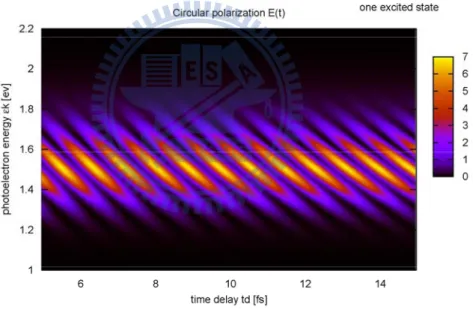
Figure. 3.8 The transition probability density _{| |}2

if

M depdents on

Chapter 4.

Considering two excited states in pump-probe model

For adding one more unbounded state, we choose the third and fourth excited state of hydrogen atom as two unbounded state, and simulate four high-harmonics orders in APT pulse. There are two unbounded state and a continuum state as intermediate state. Derive the transition probability amplitude as

s k k i t i s p p k t iE s p p k t iE if

e

M

M

e

M

M

e

e

M

M

pd pd k d L k 1 , ) ( 1 , 4 4 , 1 , 3 3 , 4 3 − −ε − τ ⋅ε +α⋅ +β −

₊

₊

_′

=

rr (4.1) To use the Fig. 4.1 to describe the mechanism for considering two excited states in pump-probe model 1s ω ω1 3p Continuum state Eenergy [ev] -13.6 -0.85 ω3 12.089 ev pump (APT) probe (IR)

+

→

4p ω2 ω4 ω 12.75 ev 0.66 ev -1.51

From the Fig. 4.1, APT contains four pulses: two pulses respectively contribute the probability for pumping an electron respectively to the |3p> and |4p>, and other pulses give the probability for ionizing an electron to the continuum state. After time delay td, the probe laser pulse coming into the system is called the second path, and contributes the probability for ionizing the electron from |3p > and |4p> respectively to continuum state and then interfere with the wave packets by first path which is by the APT pulse.

Like considering one excited state in pump-probe model, to see clarity the magnitudes and phases in the transition probability amplitude, we define that

⎪⎩

⎪

⎨

⎧

=

=

⎪

⎩

⎪

⎨

⎧

=

=

=

)

exp(

)

exp(

)

exp(

)

exp(

)

exp(

4 4 1 , 4 3 3 1 , 3 1 1 1 , 4 4 4 , 3 3 3 , p p s p p p s p s s s k p p p k p p p k

i

a

M

i

a

M

i

c

M

i

c

M

i

c

M

ϕ

ϕ

φ

φ

φ

(4.2)

Finally, the ionization probability density for two excited state in pump probe model is expressed clearly as

[

]

[

]

[

s p p L k k p d

]

s p p d p k k L p p s s p p d p p p p p p p p p p p p p p s

t

E

k

c

c

a

t

E

k

c

c

a

t

E

E

c

c

a

a

c

a

c

a

c

M

if

)

(

)

(

)

(

cos

2

)

(

)

(

)

(

cos

2

)

(

)

(

)

(

cos

2

|

|

4 4 4 1 1 4 4 3 3 3 1 1 3 3 4 3 4 4 3 3 4 3 4 3 2 4 2 4 2 3 2 3 2 1 2

−

−

+

⋅

+

−

−

−

+

−

−

+

⋅

+

−

−

−

+

−

−

+

−

+

+

+

+

=

ε

β

α

ε

τ

φ

ϕ

φ

ε

β

α

ε

τ

φ

ϕ

φ

φ

ϕ

φ

ϕ

r

r

r

r

(4.3) In RHS (right hand side) of Eqs. (4.3) , the first term is contributed by the first path which gives the probability of an electron ionizing to the continuum states by pump APT pulse, and the second and third term are contributed by the second path that produces the

from |3p> and |4p> respectively to the continuum state with the same momentum as the first path by the probe IR pulse. The first and the second path interfering with each other in the same photoelectron momentum k gives rise to the others term which are all dependent on the time delay td. We redrive the Eqs. (4.3) to the other form dependent on photoelectron angle θ_k

{

}

{

)

(

)

(

)

(

)

(

)

(

|

|

)

(

)

(

)

(

)

(

|

|

0 , 1 1 0 , 0 4 0 , 2 4 1 , 2 4 1 , 2 4 1 , 4 0 , 0 3 0 , 2 3 1 , 2 3 1 , 2 3 1 , 3 1 2 1 1 1 2 1 1 1 k i s k i p k i p k i p k i p s p k i p k i p k i p k i p s p if

Y

e

E

Y

e

D

Y

e

C

Y

e

B

Y

e

A

M

Y

e

D

Y

e

C

Y

e

B

Y

e

A

M

M

s

Ω

+

Ω

+

Ω

+

Ω

+

Ω

+

Ω

+

Ω

+

Ω

+

Ω

=

− − − β η η η η δ δ δ δ (4.4) where the coefficients are showed in Appendix A.

To integrate the transition angle-resolved probability density over photoelectron angle can find that the phase of the energy-resolved probability density P depdentent on the time _ε delay td is about (E4p −E3p)td, so the P will change with time delay tε d and the frequency is ) ( 2 3 4p E p E −

π _{≈ 6.26 fs , as showed in Eqs. (4.5) and Fig. 4.6.}

(

)

)

cos(

|

||

|

2

)

cos(

|

||

|

2

|

|

)

(

2 2 1 , 4 1 , 3 4 3 1 1 1 , 4 1 , 3 4 3 4 3 4 3 2 1 2 4 2 4 2 4 2 4 2 3 2 3 2 3 2 3 2

δ

η

δ

η

ε

ε

ε ε

−

×

+

−

×

+

+

+

+

+

+

+

+

+

+

+

=

Ω

=

=

=

∫

s p s p p p s p s p p p p p p p s p p p p p p p p k if k

M

M

D

D

M

M

C

C

B

B

A

A

E

D

C

B

A

D

C

B

A

d

M

d

dP

P

P

(4.5)

On the other hand, the probability P maybe has the same frequency with energy spectrum ε

4.1 Three-level system

For considering one more excitation state, the wave function become the superposition of hydrogen atom’s eigenstate |1s>, |3p> and |4p>

>

+

>

+

>

>=

Ψ

− − −

p

e

t

c

p

e

t

c

s

t

e

t

c

t

)

_s

(

)

i st

(

)

|

1

_p

(

)

i pt

|

3

_p

(

)

i pt

|

4

(

|

1 3 4 4 3 1 ω ω ω h h h (4.7) where h ω1s , h ω3p and h ω4p are respectively the eigenenergy of |1s>, |3p> and

> p 4

| for hydrogen atom, and the C_1s(t) , )C_3p(t and C_4p(t) are the probability amplitude of finding the electron in states |1s> , |3p> and |4p>

The external electric field contains four pulse in pump APT pulse, but only two pulse is respectively nearly resonant to the frequency for |1s> to |3p> and |1s> to |4p>. Put the Eqs. (4.7) into the time-dependent Schro&&dinger equation, so we can write down the three ordinary differential equations as

[

( 1 1) ( 2 2)

]

1 4 3 ( 2 2) 3 1 ( 1 1) 4 1

( )

1 | | 4

( )

1 | | 3

( )

2

( )

3 | |1

( )

2

( )

4 | |1

( )

2

i t i t m s p p i t m p s i t m p s

E

ic

t

e

s z

p

c

t

e

s z

p

c

t

E

ic

t

e

p z

s

c

t

E

ic

t

e

p z

s

c

t

ω ω ω ω ω ω ω ω −Δ −Δ − −Δ − −Δ

=

⋅

<

>

+

<

>

=

⋅

<

>

=

⋅

<

>

&

&

&

Figure. 4.2 △ω1=12.75 ev, △ω2=12.089 ev,

(4.5) where Em is peak value of the pump APT pulse, and <1s|z|4p> and <1s|z|3p> are the dipole moment. To carry on checking my program, we use the electric field as

ˆ

ˆ

( )

_m

cos(

)

H

′ =

E t

⋅ = ⋅

z

z E

⋅

ω ϕ

t

+

(4.6)

to check my program and there are analytical solutions for resonant frequency[3].

2 2 2 1 2 2 1 2 4 1 3 1 4 | | 1 3 | | 1 ) 2 sin( ) 2 sin( ) 2 cos( R R R R R p R p s Em p z s Em p z s t c t c t c Ω + Ω = Ω ⋅ > =< Ω ⋅ > =< Ω ⎪ ⎪ ⎪ ⎩ ⎪ ⎪ ⎪ ⎨ ⎧ Ω Ω Ω = Ω Ω Ω = Ω = ∗ ∗ (4.7)

Use the analytical solutions on resonant frequency to compare my numerical result for checking my RK4 program.

Figure. 4.3 Computing the RK4 method to compare the analytical solutions on resonant frequency, and the maximum of error is about 3.5_×10−7_{. The}

parameter respectively is E0=0.018 (a.u.), ω1=△ω1=12.75 (ev) and ω 2=△ω2=12.089 (ev)

Finally, computing the population of 3-level system for considering the Gaussian pulse shape in APT pulse is about 17.16% for |3p> state and 18.87% for |4p > state.

Figure. 4.4 The 3-level system in hydrogen atom. The thick line is the probability for finding electron at the |4p> state and the thin line is the probability for finding the electron at the |3p> state. The Peak intensity and FWHM of pump laser is 1.5×1013 _W/cm2 _{and 9 fs.}

4.2 Numerical result

Figure. 4.5 Photoelectron angle-resolved energy spectrum _{| ( )|}2

t

Mif (line-points) for

considering two excited state in pump-probe model (two-path interference model) obtained by computing the Eqs. (4.3) at the specific momentum direction θk = 3 and the time delay td = 6fs. The thin line and thick line are

respectively the 2 1 , 3 2 3 , | | | |Mk p M p s and 2 1 , 4 2 4 , | | |

|Mk p M p s , and the points

(×) is the probability density for 2 1 , |

|Mk s . The peak intensity of pump

and probe laser is 1.5×1013 _W/cm2 _{, and the FWHM of pump and probe} laser is respectively 9 and 5 fs.

Figure. 4.6 The transition energy-resolved probability density

k

d dP

ε dependents on the time

delay td. The different value between the maximum and minimum is very small because the interference term coming from the M_k,3p and M_k,4pmultiplying together, but the wave packet of M_k,3p and M_k,4p in energy domain is not the same, and one of them will be too small at a particular photoelectron energy εk.

Hence, the interference does not change so much. 6.26 fs

Figure. 4.7 The total ionization probability for considering two excited state in pump-probe model. The frequency of the probability P that repeats again is the same P_ε.

Figure. 4.8 The transition probability density _{| |}2

if

M for considering two

excited state in pump-probe model depdents on photoelectron energy εk and the time delay td at the θk = 3.

Chapter 5.

Linear and elliptical polarization effect

5.1 Linear polarization effects

For clarity, we consider only one excited state in pump-probe model to discuss the polarization effect. Rederive Eqs. (3.34) to

1 2 1 2

( , )

i

sin

i

cos

i b if l l l l

M

θ ϕ

=

A e

α

θ

+

A e

α

θ

+

Be

ϕ (5.1) where

{

}

) ( ) ( ) ( 4 3 ) cos( cos sin 4 45 0 , 1 0 , 0 3 0 , 2 2 2 1 1 1 1 2 1 2 k k i k i i l k k k bY B Y e a Y e a e A a A Ω = Ω + Ω = = − = ϕ ϕ α π ϕ α ϕ ϕ θ θ π (5.2)

In Eqs. (5.1), if θl = 0, the first term on the RHS equals zero and the term of interference

only comes from the 2nd _{term multiplying to the 3}rd _{term which coming from the first path.} However, if θl ≠ 0, the additional second term will comtribute to the interference effect.

Expand the Eqs. (5.1) to angular-resolved probability density as

2 2 2 2 2 2 1 2 1 2 2 1 1 1 2 2

|

( , ) |

sin

cos

cos(

)sin(2 )

2

cos(

)sin

2

cos(

) cos

if l l l l l b l b l

M

A

A

B

A A

A B

A B

θ ϕ

θ

θ

α α

θ

ϕ α

θ

ϕ α

θ

=

+

+

+

−

+

−

+

−

(5.3)

From Eqs. (5.3), additional terms contributing to the interference effect under the probe IR pulse without the alignment to parallel with the pump APT pulse are the

) 2 sin( ) cos( _{2 1} 2 1A l