一個無線區域網路EDCA上支援媒體串流之無接縫交遞機制

國立交通大學

資訊科學與工程研究所

碩士論文

一個無線區域網路 EDCA 上支援媒體串流

之無接縫交遞機制

A Seamless Handoff Scheme Supporting Media

Streaming on EDCA Over Wireless LAN

研 究 生 : 劉頂立

指導教授 : 陳耀宗

一個無線區域網路 EDCA 上支援媒體串流

之無接縫交遞機制

A Seamless Handoff Scheme Supporting Media

Streaming on EDCA Over Wireless LAN

研 究 生 : 劉頂立

Student : Ting-li Liu

指導教授 : 陳耀宗

Advisor : Yaw-Chung Chen

國 立 交 通 大 學

資 訊 工 程 學 系

碩 士 論 文

A Thesis

Submitted to Institute of Computer Science and Engineering College of Computer Science

National Chiao Tung University in partial Fulfillment of the Requirements

for the Degree of Master

in

Computer Science

August 2006

Hsinchu, Taiwan, Republic of China

一個無線區域網路 EDCA 上支援媒體串流

之無接縫交遞機制

研究生: 劉頂立

指導教授 : 陳耀宗

國立交通大學資訊科學與工程研究所

摘 要

A Seamless Handoff Scheme Supporting Media

Streaming on EDCA Over Wireless LAN

Student : Ting-li Liu

Advisor : Yaw-Chung Chen

Institute of Computer Science and Engineering

National Chiao Tung University

Abstract

Seamless or fast handoff schemes to support mobility of IEEE 802.11 Wireless LANs have been well developed based on the assumption that a set of next-AP/AR candidates are available prior to a handoff. A neighbor graph is one of the major strategies used to provide such information among the related studies. However, neighbor graphs have not been widely applied yet due to its inherent drawbacks. In this thesis, a so-called “discrete scan” scheme is proposed to substitute the function of a neighbor graph without drawbacks. Moreover, several mechanisms based on discrete scan are presented to help a mobile node select a desired next AP to handoff to. The analytical model and simulation are elaborated to show performance of the approaches. Discrete scan may bring concerns on its impact to received QoS of the mobile node. However, the simulation results show that disruptions caused by discrete scan can be controlled within an acceptable value for a media streaming device working under EDCA over wireless LAN.

Acknowledgement

I would like to express my sincerity to the Prof. Yaw-Chung Chen for guiding

this thesis and giving me some practical suggestions. Besides, I appreciate very much

for help and advice from all members in multimedia communications laboratory,

Table of Contents

摘要 ……….. i

Abstract ……… ii

Acknowledgement ………... iii

List of Figures ……….. vi

List of Tables ………vi

Chapter 1 Introduction………1

Chapter 2 Related works ……… 7

2.1 Review of Layer-2 And Layer-3 Handoffs ………. 8

2.1.1 IEEE 802.11 Handoffs ……… 8

2.1.2 Mobile IP Handoffs ……… 9

2.2 Fast Handoff Schemes Based on Next AP/FA Prediction……… 12

2.2.1 AP Probe Latency ………. 12

2.2.2 Association Latency……….. 12

2.2.3 802.1x Authentication Latency………. 13

2.2.4 Layer-3 Handoff Latency……….. 13

2.2.5 Cross-Layer Design ……….. 13

2.3 Summary of Related Works………... 14

Chapter 3 Proposed Approaches………. 15

3.1 Discrete Scan Scheme……… 15

3.2 Collection of Next-AP candidates ………... 18

3.3 Mechanisms to Select a Next AP………. 21

3.3.1 Mechanisms to Select the Nearest AP……….. 21

3.3.2 Setting of a Sniffing Period ………. 25

3.3.4 Select Best Next AP Instead of the Nearest AP……… 35

3.4 Impact on Service QoS……….. 36

Chapter 4 Performance Evaluation ……… 42

4.1 Simulation Environment……… 42

4.2 Station Count Mechanism in EDCA Environment……… 44

4.2.1 Setting of a Sniffing Period in EDCA Environment………. 44

4.2.2 Performance of Station Count Mechanism in EDCA Environment…….. 47

4.3 Impact on Service QoS in EDCA Environment……… 51

Chapter 5 Conclusion and Future Works ……….. 53

List of Figures

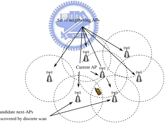
Figure 1.1 Set of neighboring APs and set of next-AP candidates by discrete scan... 6

Figure 2.1 Overall latency in a layer-2 and layer-3 handoff... 11

Figure 3.1 Scheme for wireless NIC in pre-handoff periods ... 17

Figure 3.2 Three kinds of evidences to discover an AP ... 18

Figure 3.3 Example sniffing scheme in the environment of 3 channels ... 20

Figure 3.4 the higher station distribution ratio indicates the nearer AP ... 22

Figure 3.5 The station counts in two BSSs... 24

Figure 3.6 Definition of Ts and Tc, slot time of transmission with success and collision ... 27

Figure 3.7 Transient number of stations (r) v.s. number of stations (n) for different Tsniff values ... 29

Figure 3.8 Scenario for performance estimation ... 32

Figure 3.9 Hit ratios v.s. distances in balanced number of stations... 33

Figure 3.10 Variation of hit ratios with imbalance of number of stations ... 34

Figure 3.11 Total disruptions induced with a discrete scan... 38

Figure 3.12 Probability to transmit a frame in 10 ms v.s. number of stations in a BSS ... 41

Figure 4.1 Simulation configuration... 43

Figure 4.2 Number of transient stations v.s. number of stations in EDCA of 70% TCP and 30% VoIP nodes... 45

Figure 4.3 Number of transient stations v.s. number of stations in EDCA with 100% TCP nodes... 46

Figure 4.4 Hit ratios v.s. distances in balanced number of stations in EDCA WLAN of 30% VoIP nodes and 70% TCP nodes. ... 47

Figure 4.5 Hit ratios v.s. distances in balanced number of stationsin EDCA WLAN of 100% TCP traffic ... 48

Figure 4.6 Hit ratios v.s. imbalanced number of stations in EDCA of 30% VoIP nodes and 70% TCP nodes... 49

Figure 4.7 Hit ratios v.s. imbalance of number of stations in EDCA of 100% TCP traffic... 50

Figure 4.8 Probability to send a frame in 10 ms v.s. number of stations in 11 Mbps EDCA wireless LAN... 52

List of Tables

Chapter 1 Introduction

In recent years, wireless LANs have been widely deployed for public mobile Internet services. Public wireless LANs can provide high-speed Internet connectivity using portable devices such as laptop computers and personal digital assistants (PDA). An emerging application to wireless LAN system could be Voice over IP (VoIP), which requires networks to support real-time transmission such as bounded latency and jitter. One of the key issues for VoIP application to support real time servise is providing the Quality of Service (QoS) that meets the user expectations. This is recognized as the single biggest challenge in providing high-quality voice on wired IP-based networks. In wireless networks, one of the major issues affecting QoS is to minimize the service disruption during handoffs of the mobile nodes.

It is recognized that an intra-subnet handoff across access points (APs) in an administrative domain, so-called layer-2 handoff, normally brings a service disruption of several hundreds of mini-seconds (ms), and an inter-subnet handoff across different domains, so-called layer-3 handoff, would be disrupted in periods of several seconds. However, to meet the requirement of real-time services, the maximum latency would be limited to less than 100 ms. Therefore, lots of investigation devoted to minimizing the handoff latency, which is defined as the period while a mobile node is unable to receive application traffic due to the handoff.

Among the researches focusing on minimization handoff latency, schemes based on prediction of next AP for a layer-2 handoff, or next access router (AR) for a layer-3 handoff are proposed in lots of literatures. Neighbor graphs, which are defined as a specific data structure that stores information of set of neighboring APs or/and ARs with respect to current AP or/and AR, are one of major approaches to predict

next APs or/and ARs to handoff to. With aids of neighbor graphs, mobile nodes in a layer-2 handoff will probe the channels in which at the least one of the neighboring APs exists. Moreover, mobile nodes can terminate probing the channel immediately after the last neighboring AP has responded rather than wait until maximum channel time. Therefore, the probe phase in layer-2 handoffs can be significantly shortened with the help of neighbor graphs [1].

The reassociation latency in layer-2 handoffs can be reduced an order by the scheme that the current AP caches secure information of mobile nodes to all of the APs in neighbor graphs prior to occurrence of layer-2 handoffs [2]. The 802.1x reauthentication to new AP would also bring significant latency to layer-2 handoffs. By means of proactive key distribution to all of the APs in neighbor graphs are reported to effectively eliminate the 802.1x reauthentication latency from 800 ms up to 10 ms [3].

The layer-3 latency can be effectively reduced to a level of layer-2 handoffs with aids of neighbor graphs. The neighbor-casting scheme sets up temporary links from current AR to all ARs in neighbor graphs in order to maintain the connection to the mobile node via the relay of current AP to next AP in a layer-3 handoff. Therefore, the latency induced by a layer-3 handoff is eventually reduced to the same level as disruptions caused by the layer-2 handoff [4].

The neighbor graphs include information of all possible APs/ARs that a mobile may handoff to from the current AP/AR. The size of a neighbor graph (i.e., number of APs/ARs in a neighbor graph) may be large enough to cause severe overhead to wired networks. Size of a neighbor graph reflects the number of potential APs to be probed for a mobile node to complete the probe phase in a layer-2 fast handoff. In both context caching and neighbor-casting schemes, the context of the mobile node and the arriving packets for the mobile node during a layer-3 handoff have to be duplicated as

many copies as the number of APs/ARs in neighbor graphs. Therefore, the size of a neighbor graph stands for the overhead to wired bandwidth in a fast handoff scheme. In proactive key distribution scheme, the pairwise master keys (PMK) are generated and distributed to all APs in neighbor graphs. The size of a neighbor graph thus responds to the overhead and the security risk caused by abuse of key distribution.

To reduce the size of a neighbor graph, some schemes such as selective neighbor caching [5] and frequent handoff region (FHR) [6] are proposed. Moreover, global positioning system (GPS) is proposed to update the topology information of a mobile node dynamically for the sake of predicting the next AP among APs, in a neighbor graph before a handoff is initiated. Based on the assumption that next AP and next AR are known prior to the occurrence of a handoff with aids of a neighbor graph and real time topology information, a cross-layer fast handoff scheme is proposed to minimize overall latency for a layer-2 and layer-3 handoff to less than 50 ms in the experiment results [7].

It is generally recommended to configure a neighbor graph with a distributed manner such that each AP/AR stores and maintains its own neighbor graph. The neighbor graph can be automatically learned by the individual AP/AR with the reassociation frames and registration packets from various mobile nodes. Distributed neighbor graphs require the supports from neighboring APs/ARs as well as the mobile nodes roaming through the coverage of APs/ARs.

In fact, not all of the mobile nodes have to invoke for seamless handoffs. For example, a laptop with a wireless network interface card (NIC) may be considered as a mobile node since it may be carried from the coverage area of an AP/AR to another. With its volume and weight, the user may seldom play real time application (such as VoIP) while the laptop is being carried across different wireless LAN. Therefore, seamless handoffs may be not a mandatory function for a laptop with wireless NIC

unless the notebook is especially designed for used in a vehicle. A hand carried device such as personal digital assistants (PDA) may run only in non-real-time applications, such as web browser or specific remote database queries. A hand held device for non-real-time applications may neither need feature of seamless handoffs since disruptions of few hundreds mini-seconds is generally tolerable to users. A typical example that really invokes for seamless handoffs is recognized as media streaming, such as a WiFi VoIP, with both attributes of hand held devices and real-time application. Since only particular clients request for seamless handoffs, neighbor graph scheme may induce unnecessary overhead by non-seamless-handoff nodes because neighbor graph scheme is implemented in AP that provides universal service to all of its clients. For example, a stationary station may work as a client of an AR with neighbor graph function. By ignoring the non-seamless-handoff attribute, an AR may buffer and forward the packets to all its neighboring ARs in case a sudden termination from the client is misinterpreted as an event of handoff, so that misinterpretation as well as bandwidth waste may occur.

Millions of IEEE 802.11 APs/ARs as well as mobile nodes have been deployed without supports to neighbor graphs. One of the reasons for the popularity of IEEE 802.11 wireless LAN is due to the features of simple configuration and low cost. To support neighbor graph mechanism, unfortunately, increases complexity and cost to re-configure an IEEE 802.11 wireless LAN. Moreover, a new protocol will be required to enable cooperation among APs/ARs and mobile nodes though some of mobile nodes do not require seamless handoffs from wireless circumstance.

The factors described above somehow explain the difficulty for neighbor graph mechanism to be implemented in existed wireless networks, though researches have proven with experiments that seamless inter-subnet handoffs can be eventually achieved with integral fast handoff schemes benefit by neighbor graph mechanism.

In this thesis, the so-called “discrete scan”, a simple and effective scheme to collect the set of potential next APs in a layer-2 handoff is proposed. A mobile node with discrete scan scheme executes the process of passive scan a certain time ahead of handoff initiation. To avoid disruptions lasting longer than 50 ms, process of passive scan is divided into smaller pieces of sniffing periods; therefore, the probe delay in layer-2 handoff is decomposed into pieces of disruption that users are unable to sense. Discrete scan is designed to implement in a media streaming application such as WiFi VoIP that typically desires function of seamless handoffs. Benefit by features of dedicated hardware and relative low working bit rate (usually less than 100 Kbps bidirectional) compared with its network interface card (NIC) (11Mbps), discrete scan scheme can take place of neighbor graphs without collaboration from APs as well as other mobile nodes.

The characteristic that a mobile node spends its own effort to predict the next AP to fasten its handoff may allow the seamless handoff schemes to utilize to discrete scan. Without any support from AP, the mobile nodes using discrete scan can perform a fast handoff by elimination of probe latency from a layer-2 handoff. The confusion for an AP to provide a seamless handoff service to a node without such demand can be avoided because discrete scan will be only implemented in the nodes that may invoke seamless handoffs.

Compared with neighbor graphs, the set size of candidate next-APs collected by discrete scan scheme is much smaller than that by neighbor graphs. As shown in Figure 1.1, discrete scan scheme discovers only a subset of neighboring APs of which signals can reach to the mobile node. Taking advantage of examined information from frames received in discrete scan, such as received signal strength (RSS), MAC address and network allocation vector (NAV), several mechanisms to assist the mobile node to select the nearest or/and the best AP among the candidates is

introduced in this thesis.

With discrete scan as well as its auluxiary mechansims, the mobile node is able to select the most appropriate AP to handoff to before handoff is initiated. Thus, latency induced by probe phase in a layer-2 handoff is significantly reduced to a ProbeRequest from the mobile node and a ProbeResponse from the selected AP, without modification to the existed infrastructure of IEEE 802.11 wireless LANs. Since the latency spent in probe phase is recognized as more than 90% of overall layer-2 handoff latency, discrete scan with its auluxiary mechansims expect to reduce 90% of latency in a layer-2 handoff. With such significant improvement but without modification required to the current system, the realization of discrete scan scheme for a mobile node is reasonably much easier than that of neighbor graph scheme.

Set of neighboring APs

Current AP

Candidate next-APs

discovered by discrete scan

Figure 1.1 Set of neighboring APs and set of next-AP candidates in discrete scan.

Discrete scan is supposed to support seamless layer-3 handoffs with the fast handoff schemes proposed for neighbor graphs. Substituting for the functions of a

neighbor graph and its extensions, discrete scan with auxiliary mechanisms proposed in this thesis helps a mobile node determine the next AP in advance of the trigger of a handoff. The only insufficiency for discrete scan scheme to take place of a neighbor graph lays on the lack of the ability to discover next AR because discrete scan is absolutely designed for layer-2 operation. However, a lookup table built-in the current AP, that outputs next AR with input of the next AP, will simply address the problem.

One of major concerns on discrete scan scheme is its impact on the service QoS received in the periods of discrete scan, because discrete scan decomposes the latency of probe phase in a layer-2 handoff into pieces. Benefit by the high transmission priority of VoIP traffic in wireless EDCA environment, the simulation results in this thesis show that QoS degradation due to discrete scan is controlled within a tolerable value for a real-time application.

The rest of this thesis is organized as follows. Chapter 2 introduces the background of latency in layer-2 and layer-3 handoffs. The relative works involved in neighbor graphs are introduced briefly in this chapter as well. In Chapter 3, we elaborate discrete scan scheme and the mechanisms to select next AP. Besides, in Chapter 3, the performance and impact on service QoS are evaluated by numerical results based on analytical model of DCF wireless LAN environment, and those in EDCA environment are demonstrated with simulation results in Chapter 4. Finally, the conclusion and future works are presented in Chapter 5.

Chapter 2 Related works

In this chapter, we first briefly review the processes of a layer-2 handoff and a layer-3 handoff as those extracted from [7]. IEEE 802.11 wireless LAN and mobile IP (MIP) standard are interpreted as typical samples for a layer-2 handoff as well as a layer-3 handoff.

Next to review on handoff process, the breakdown latency for a layer-2 and a layer-3 handoff is presented as those proposed in [7]. References in this section show that each division for handoff latency can be significantly reduced based on the aids of neighbor graphs that provide current AP/AR and the mobile node a set of neighboring APs/ARs that contains the next AP/AR in a handoff.

Finally we conclude that the capability to predict next APs/ARs in advance of a handoff is the key point to fulfill a fast handoff. A new scheme for a mobile node to predict or select the next AP/FA in a handoff is proposed in this thesis to replace the function of a neighbor graph. The proposed scheme in this thesis will be able to work with the strategies designed for working with a neighbor graph. A series of fast handoff studies based on the existence of a neighbor graph are addressed in section 2.2.

2.1 Review of Layer-2 And Layer-3 Handoffs

2.1.1 IEEE 802.11 Handoffs

A layer-2 handoff consists of three phases: probe, authentication, and reassociation. In the probe phase, a mobile node discovers next-AP candidates

through either an active or a passive scan. In an active scan, a mobile node broadcasts through a selected channel a ProbeRequest message with a particular Service Set Identifier (SSID). If the SSID matches an AP’s configuration, then the AP responds with a ProbeResponse to the mobile node, and the mobile node can therefore be made aware of the presence of the AP. If the mobile node instead uses a passive scan, then it does not issue any message but listens to Beacon messages broadcast periodically by APs on channels of interest.

With AP information obtained from the ProbeResponse or Beacon message, the mobile node selects a new AP to camp on based on the measure of received signal strengths. Following the probe phase, the mobile node performs 802.11 authentication (open system or WEP), and then reassociation phases with the newly selected AP. In the authentication phase, the mobile node exchanges 802.11 authentication messages with the AP. In the reassociation phase, the mobile node sends a ReassociationRequest to the AP and receives a ReassociationResponse replied by the AP. The receipt of the last message terminates the 802.11 handoff process.

As a port-based network access protocol, IEEE 802.1x provides authentication and key management under various 802 LAN infrastructures, and is now extensively adopted in 802.11 WLANs to resolve the limitations of WEP. An 802.1x-enabled AP acts as an authenticator controlling the mobile node’s access to the Internet. The authenticator communicates with an authentication server that makes authorization decision on the access requests sent by a mobile node (called a supplicant in 802.1x terms). Either the mobile node or the authenticator may initiate an 802.1x authentication immediately after the reassociation phase is completed. If the authentication is successful, then the authentication server sends a pair-wise master key (PMK) to the authenticator, which then initiates an 802.11i four-way handshake procedure to synchronize the PMK with the mobile node and to generate pair-wise

temporal keys (PTKs). The 802.1x control port of the authenticator is then unblocked for the mobile node, and the mobile node can then send and receive messages protected by the PTKs.

2.1.2 Mobile IP Handoffs

Mobile IP (MIP) is an Internet standards track protocol that enhances the existing IP protocol to accommodate host mobility. In MIP, a special host called a mobility agent (MA) maintains registration information for mobile nodes. When a mobile node moves away from its home network, the MA located in the mobile node’s home network, called the mobile node’s home agent (HA), tunnels packets for the mobile node. A mobile node away from its home network can retain its connection to the Internet aided by the HA and the FA.

MIP facilitates care-of address (CoA) to identify a mobile node in the visited network. As a mobile node registers a CoA with the mobile node’s HA, then the FA intercepts all tunneled packets destined for the mobile node, and delivers then to the mobile node. When a mobile node detects that the current FA (cFA) is no longer accessible, it initiates a layer-3 handoff from the cFA to the next FA (nFA). A layer-3 handoff consists of two phases: the mobile node must first discover the nFA and then register with the mobile node’s HA through the nFA, as described below:

a. Agent Discovery: This concerns how a mobile node becomes aware of the presence of an nFA. Every MA can be uniquely identified by its AgentAdvertisement message. A mobile node may either passively listen to AgentAdvertisement messages broadcasted periodically by the nFA, or actively issue an AgentSolicitation message to request an advertisement.

b. Registration: This informs the HA of a mobile node’s CoA. The mobile node issues a RegistrationRequest message to the nFA, from which the message is then forwarded to the HA. The HA sends a RegistrationReply to the mobile node to confirm the registration with relay of the nFA.

The process through which a mobile node detects that a cFA is no longer accessible is called move detection. MIP specifies two move-detection principles: the advertisement expiration and the network prefix change. Each AgentAdvertisement in MIP carries an advertisement lifetime. If the lifetime of the most recently received advertisement expires, then the mobile node may assume that the cFA is unreachable, which generally leads to long move detection delays, as MIP suggests that the advertisement lifetime should be long enough to tolerate three consecutive losses of advertisements. Alternatively, if the mobile node receives an AgentAdvertisement with a network prefix different from that of the mobile node’s current CoA, then the mobile node may deduce that cFA is unreachable, leading to a long move-detection delay as the mobile node can receive nFA’s advertisement only after a layer-2 handoff.

2.2 Fast Handoff Schemes Based on Next AP/FA Prediction

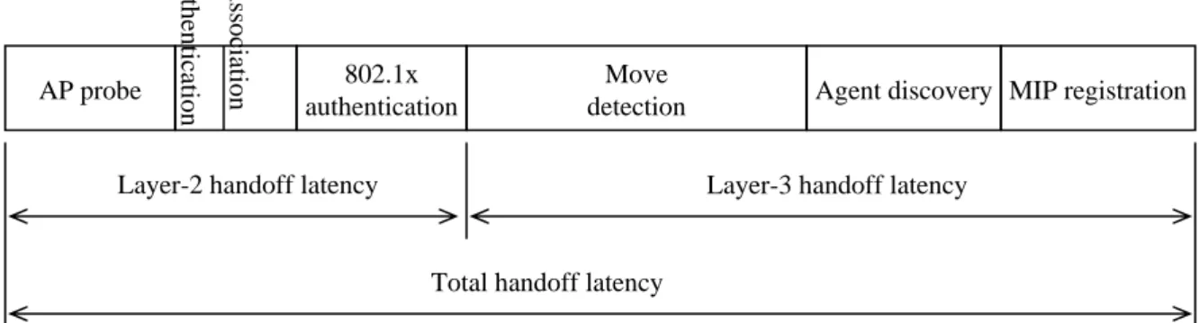
AP probe 802.1x

authentication Agent discovery Move

detection MIP registration Layer-2 handoff latency

Total handoff latency

Layer-3 handoff latency

Ass o ciation th en tication Au

Figure 2.1 illustrates total latency incurred in layer-2 and layer-3 handoffs. Many studies have attempted to reduce the delay in different activity sections to shorten handoff latency, as described in following subsections.

2.2.1 AP Probe Latency

In [1], Mishra et al. have noted with experiments that AP probe phase latency significantly contributes to the layer-2 handoff latency, and recommended using neighbor graphs to eliminate the delay in AP probe. The mobile node only needs to probe the neighboring APs with respect to the current AP. An AP is a neighbor of another AP only if a handoff from the latter to the former has occurred recently. Neighbor graphs thus dynamically capture temporal handoff-to relationships.

2.2.2 Association Latency

Mishra et al. [2] have also facilitated neighbor graphs to lower the reassociation latency by proactively caching security information to neighboring APs, where security information is needed to establish secure communication channels between APs. The experiment results show reassociation latency could be reduced from 15.37 ms to 1.69 ms if the mobile node’s context has been cached to the next AP prior to a handoff. To reduce the costly signaling overhead brought by proactive neighbor casting, Sangheon Pack [5] recommended only the neighboring APs with relative high probabilities that a mobile node may handoff to be selected as next-AP candidates.

2.2.3 802.1x Authentication Latency

Exploiting a neighbor graph as well as proactive key distribution to candidate set of next APs with which a mobile node may reassociate, the 802.1x reauthentication latency incurring in layer-2 handoffs is reduced down to 50 ms with comparison to 800 ms for a full 802.1x authentication [3].

2.2.4 Layer-3 Handoff Latency

Several schemes such as neighbor casting [4], centralized decision engines [9], and Frequent Handoff Region [6] have been proposed to collect sets of next-FA candidates. In the neighbor-casting scheme, the current FA sets tunnels to all of the next-FA candidates for the purpose to relay packets for a mobile node after it losses its connection to the mobile node caused by a layer-3 handoff. With such a mechanism that the cFA buffers-and-forwards packets to nFA for the mobile node, the latency brought with a layer-3 handoff is eliminated to the level as a layer-2 handoff [8].

2.2.5 Cross-Layer Design

It is proposed to take advantage of neighbor graphs and topology information offered by auxiliary equipment such as Global Position System (GPS) to derive an accurate prediction on next FA in a layer-3 handoff. Move detection and agent discovery delay in a layer-3 handoff are minimized by post handoff trigger scheme because next FA has been known before the handoff. Further, registration for the

predicted next FA to HA could be done before layer-3 handoff occurs, called pre-handoff trigger scheme. Therefore, the total latency for layer-3 handoffs is eliminated to its minimum with a cross-layer design fast handoff scheme in [7]. Experiment results in [7] show that cross-layer design with the supports of accurate prediction of the next AP reduces overall end-to-end layer-3 handoff latency up to 50 ms so that a seamless layer-3 handoff can be achieved.

2.3 Summary of Related Works

A series of fast handoff studies have been developed based on the hypothesis that the information of the next APs/FAs is collected or predicted to somewhat degree by a particular mechanism. The neighbor graph [1] [2] [3] [4] [7] is one of the major mechanisms utilized to provide information of a set of the next-AP/FA candidates. To further improve accuracy of prediction or reduce the number of next-AP candidates, some enhancement such as design engine [5] and frequent handoff region [6] are presented. The ultimate prediction mechanism that aims on the ability to detect exactly the next AP or/and AR prior to handoffs initiated was proposed to take advantage of a neighbor graph with aids of topology information updated by a GPS in the mobile node [7]. It concludes that the support to know the next AP/AR in an impending handoff is the key to minimize an overall latency, because a series of fast handoff schemes based on known next AP/AR have been presented with experiment results.

Chapter 3 Proposed Approaches

In this chapter, we propose a so-called “discrete scan” scheme and relative auxiliary mechanisms that collect a set of candidates for next-APs and eventually select the next AP for a mobile node before a forthcoming handoff. Moreover, various existed mechanisms may select next AP with different properties of the next-AP candidates, such as the nearest AP, the approached AP, the AP of highest available bandwidth, or their combination.

Compared with neighbor graphs, discrete scan scheme provides a set of next-AP candidates as a subset of neighboring APs. With the help of proposed auxiliary mechanisms, discrete scan selects an appropriate next AP for a mobile node to handoff to, taking the place of the function of a neighbor graphs with aids of topological information by GPS system proposed in [7].

As a cost, discrete scan scheme contributes an impact to service QoS received by the mobile node in a “pre-handoff” period that is defined as the duration from initiating the discrete scan scheme to the moment when a handoff is initiated. However, taking the advantages of high transmission priority and relative low bit rate for a VoIP connection in EDCA wireless LANs, the degradation may be limited to a degree that the users may tolerate or even may ignore. Estimation on the QoS degradation with analytical approach and simulation results presented in this and next chapter shows that the disruptions caused by discrete scan are bounded to 50 ms based on certain practical assumption.

The main idea of discrete scan is to allow a mobile node utilizing idle time of its wireless NIC to survey its wireless environment in the periods about to handoff. As described in Chapter 1, only hand carried sets in real-time application, typically as WiFi phones, in fact require seamless handoffs in IEEE 802.11 wireless environment. A hand held device normally implies a dedicated hardware that allows modification of firmware and even its hardware to meet particular requirements. Real-time applications usually work in relative low bit rates with respect to the available bandwidth of its wireless NIC. Taking a WiFi VoIP service as a example: the WiFi phones operate with bidirectional traffic both with 64Kbps constant bit rate (CBR) in an IEEE 802.11b wireless LAN which supports at the least 2 Mbps half duplex bandwidth. From the viewpoint of the wireless NIC of a WiFi phone, traffic transmission and receiving time takes about 64K*2 / 2M = 6.4% of total operation time. More time may be taken by transmission overhead such as physical layer overhead, MAC header, MAC layer control frames, waiting time for media contention, retransmission due to collisions, etc, however, NIC keeps in idle status for a significant portion of time.

In discrete scan, a mobile node, such as a WiFi phone set, will make use of the idle time in pre-handoff duration to sniff its wireless environment to collect a set of next-AP candidates for a forthcoming handoff. A pre-handoff period is initiated with an event that received signal strength (RSS) from current AP is detected to be lower than a preset threshold δ2 for a preset period. Obviously, threshold δ2 shall be set a

little bit larger than the threshold δ1, the threshold RSS to initiate a layer-2 handoff in

IEEE 802.11.

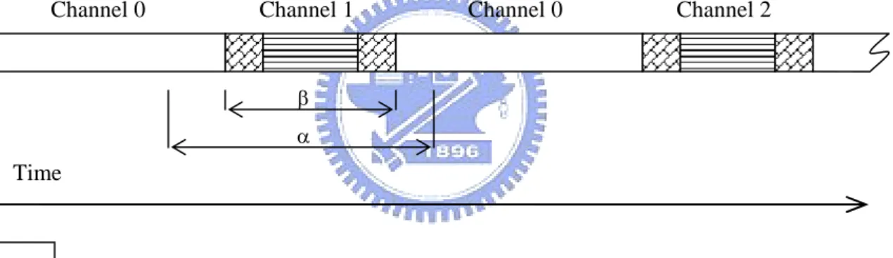
In the pre-handoff periods, the wireless NIC of a mobile node operates in a mode that switches channels with specific scheme. Figure 3.1 below illustrates the typical scheme for the wireless NIC in the pre-handoff periods. While working in pre-handoff

mode, the wireless NIC has to return to working channel to maintain VoIP connection alive with a certain level of QoS. The time between two working periods, that is, the time of sniffing period plus two switching periods, should not be longer than β ms so that the maximum latency allowed by a real time application, α ms, is maintained if the node will get at least two times of transmission within (α−β) ms, as shown in Figure 3.1. During working periods, bidirectional traffic transmits between current AP and the mobile node at least once to deliver the traffics generated in previous absence from working channel. By the end of working periods, the mobile node should issue an extra control frame of power save mode (PSM) to notice the current AP to suspend the packets for the mobile node.

Figure 3.1 Scheme for wireless NIC in pre-handoff periods

In principle, discrete scan amortizes the latency for probe phase in a layer-2 handoff with pieces of sniffing periods in a pre-handoff duration. Each sniffing period should be short enough in order to maintain the induced disruption within tolerable limits for a real time application. The setting of the length of sniffing periods will sometimes become a trade-off between efficiency of collecting next-AP candidates

Working periods: The periods for Tx/Rx in the working channel (channel 0) Channel 1

Switching periods: The time for wireless NIC to switch channel Sniffing periods: The periods for sniffing channels (channel 1~10)

Channel 2

Time

Channel 0 Channel 0

α β

and degradation of service QoS in a pre-handoff period.

3.2 Collection of Next-AP Candidates

To substitute for the function of neighbor graphs, discrete scan must be able to collect a set of next-AP candidates. One of the natures particular to a seamless handoff is that a mobile node must have entered the coverage area of its next AP before a layer-2 handoff is triggered. Therefore, a mobile node can discover the entire set of next-AP candidates by means of sniffing frames transmitted from APs in various channels. Note that the number of next-AP candidates discovered by discrete scan scheme is much less than the number of neighboring APs because only those neighboring APs located at the area that the mobile node can listen to can be found (refer to Figure 1.1).

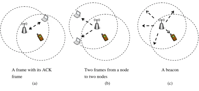
In Figure 3.2, there are three kinds of evidences to identify the discovery of a next-AP candidate, as described in the following:

Figure 3.2 Three kinds of evidences to discover an AP A frame with its ACK

frame

(a)

Two frames from a node to two nodes

(b)

A beacon (c)

a. A complete transmission with both of data frame and corresponding ACK frame is sniffed. In this case, it is inferred that a next-AP candidate and one of its clients locates within the area the mobile node can listen to. In case none of active stations locate in the coverage of the mobile node, the AP will not be found under this condition.

b. Two frames sent from a node (of the same MAC address) to different destinations are sniffed. By the nature of infrastructure wireless LAN, only the AP of a basic service set (BSS) can send frames to different destinations, so that the sender of two frames to distinct receivers will be identified as an AP. Since the frames from AP have been sniffed, the mobile node must be locating within the coverage of the AP, therefore, the AP is recognized as one of candidate next AP. If a BSS has less than two active stations in sniffing periods, the next-AP candidate will not be found under this condition.

c. A beacon is sniffed, same as a traditional scheme to identify an AP. Because a sniffing period is shorter than a beacon interval, there is no guarantee that all of next-AP candidates will be found in a sniffing period. However, utilizing the convention that all the beacon intervals are typically set as 100 ms, each beacon interval may be considered as multiple time slots with each slot equal to a sniffing period. A mobile node may discover all of its next-AP candidates in different channels through their beacons, in case it separately sniffs all the time slots for each channel.

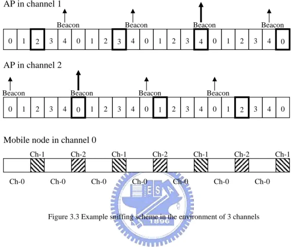
An example design for the sniffing scheme is illustrated in Figure 3.3. A sniffing period is designated by 20 ms for each interval of 60 ms. Assume that only three channels are deployed in the concerned area. A beacon interval is consisted of 5 slots, from slot 0 to slot 4, with each slot time 20 ms, and two channels that are different

from the working channel will be listened in a sequence of sniffed periods. The sniffed channels should be interleaved so that each channel is probed evenly.

0 1 2 3 4 Beacon

0 1 2 3 4 0 1 2 3 4 0 1 2 3 4 Beacon Beacon Beacon

0 1 2 3 4 Beacon

0 1 2 3 4 0 1 2 3 4 0 1 2 3 4 Beacon Beacon Beacon

0 0 Ch-0 Ch-0Ch-0 Ch-0 Ch-2 Ch-1 Ch-0 Ch-0 Ch-0 Ch-2 Ch-1 Ch-2 Ch-1 Ch-1 AP in channel 1

Mobile node in channel 0 AP in channel 2

Figure 3.3 Example sniffing scheme in the environment of 3 channels

The maximal time required for a mobile node to discover all APs through beacons should be taken into account to set the value of δ2, the threshold RSS to start

a pre-handoff period. As an example, 20 ms slot of each 60 ms interval is used for sniffing, that is, 1/3 of total run time is shared to sniff for the next-AP candidates in all channels except the working channel. Each scanned channel takes 5 sniffing periods, equal to 100 ms in total, to ensure to discover of all of the next-AP candidates active in the channel. Therefore, it takes (number of channels–1) * 3 * 100 ms to complete the discrete scan scheme on all of channels. With at the most 11 channels in IEEE 802.11b wireless LAN environment, thus, it takes (11-1) * 3 * 100 ms, equal to 3 sec, to complete a full passive scan. Therefore, a pre-handoff period is suggested to be 3 seconds ahead of a layer-2 handoff.

3.3 Mechanisms to Select a Next AP

3.3.1 Mechanisms to Select the Nearest AP

Discrete scan surpasses the neighbor graph in the ability to select a much suitable next AP for a mobile node before the handoff starts. Taking the advantage of the information extracted from MAC frame headers that a mobile node listens through its discrete scan scheme; a desired next AP can be determined by the mobile node along with extra supports from existed wireless LAN system. The feature to determine the next AP may take over the function of a neighbor graph with aids of GPS as proposed in [7].

The nearest AP is normally chosen as the next AP in a handoff because of property of the best signal strength. In a conventional handoff schemes, a mobile node determines the nearest AP by the RSS received from beacons or frames sent by APs during the probe phase of a layer-2 handoff. However, it is recognized that the strongest RSS may be not a prefect indicator of the nearest AP because of the effects by multi-paths interference of microwave communications. Nevertheless, the principle of choosing the next AP by indication of RSS is widely implemented in wireless NIC, since no better indicator is available so far.

Discrete scan, discovering next-AP candidates through frames or beacons sent by APs, may restrict the capability to select next AP by their RSS. Furthermore, several mechanisms of a new idea with aids of MAC layer information are proposed in this section to compensate the insufficiency of RSS scheme currently supported by physical layer.

A mobile node with discrete scan may derive information to indicate the next AP of the handoff by the MAC headers in the frames listened in its sniffing periods. By

reading MAC layer headers, a mechanism is designed to record the number of stations that can be listened by the mobile node in each channel. A mobile node learns a station with its MAC address in the frame header transmitted from the station.

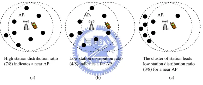
The first proposed mechanism for a mobile node to estimate its distances from candidate APs is named “station distribution ratio” that is defined as the ratio of the numbers of stations of in the coverage of the mobile node to all of the stations in a BSS. As illustrated in Figure 3.4(a) (b), the higher station distribution ratio is a BSS, the nearer is the AP to the mobile node.

Figure 3.4 the higher station distribution ratio indicates the nearer AP.

The key mechanism of station distribution ratio lies in how a mobile node distinguishes a station within its area from those out of its area in a BSS. By reviewing the Figure 3.2(a) once more, a mobile node can identify a station in its coverage area if the mobile node can receive both a data frame and the corresponding ACK frame in its discrete scan scheme. Similarly, if a mobile node receives only one of a data frame or the corresponding ACK frame, as illustrated in Figure 3.2 (b), the mobile node infers that the station in the BSS locates out of its coverage.

Another good feature that discrete scan surpasses neighbor graphs is its slight

AP1

High station distribution ratio (7/8) indicates a near AP.

(a)

AP2

Low station distribution ratio (4/8) indicates a far AP.

(b)

AP1

The cluster of station leads low station distribution ratio (3/8) for a near AP

penalty if an incorrect AP is selected by the auxiliary mechanisms. A mobile node always locates at the overlapped coverage of all of the next-AP candidates discovered in the discrete scan scheme, therefore, an improper selection among the next-AP candidates will not lead to a failure of a handoff. On the contrary, a mobile node will lose connection if the GPS in a mobile node predicts a neighboring AP that can not reach to the mobile node as the next AP.

As illustrated in Figure 3.4(c), the cluster of stations in a BSS may lead the station distribution ratio mechanism to an improper selection of the next AP. However, the penalty for a mobile node to handoff to a farer AP may just cause another handoff to occur earlier.

There are some shortcomings of the station distribution ratio mechanism. The station distribution ratio mechanism will be active only after an AP is discovered because a mobile node infers a station out of its coverage by frames from AP instead of the station. Consequently, the station distribution ratio mechanism requires a certain amount of time to evaluate an AP after it is discovered. Besides, a mobile node needs more extra cache to memorize the MAC addresses of discovered stations to avoid counting a station twice.

To overcome the drawbacks described above, the station distribution ratio mechanism is simplified and submitted as the second mechanism for a mobile node to select the nearest AP among candidate APs. The mechanism is named as “station count” because it suggests a mobile node to select an AP with the largest number of stations counted by a mobile node in the last sniffing period prior to a handoff. A mobile node with station count mechanism updates the number of stations it found in a BSS in each short sniffing period (e.g., 20 ms) of a discrete scan scheme. Because the mobile node concerns only the stations that locate in its coverage area and transmit at least one frame in a short sniffing period, much less cache memory is

needed to keep MAC addresses of discovered stations, and a simple algorithm that collects the frames of various senders to a receiver is sufficient to identify an active station in the coverage. Furthermore, a mobile node starts to sense a BSS before it enters the coverage; therefore the evaluation of a BSS is available with discrete scan once its AP is discovered by the mobile node.

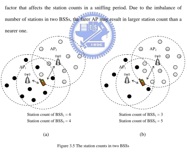
As illustrated in Figure 3.5(a), the nearer is the mobile node to an AP, the larger overlapped coverage the mobile node can listen, and consequently the mobile node can discover more active stations in a sniffing period. Unfortunately, the distance between a mobile node and an AP is not a unique factor that affects the station counts. As illustrated in Figure 3.5(b), the total number of stations in a BSS is another major factor that affects the station counts in a sniffing period. Due to the imbalance of number of stations in two BSSs, the farer AP may result in larger station count than a nearer one. (a) (b) AP2 Station count of BSS1 = 6 Station count of BSS2 = 4 AP1 AP2 AP1 Station count of BSS1 = 3 Station count of BSS2 = 5

Figure 3.5 The station counts in two BSSs (a) The larger station count maps to the closer AP.

The third factor that affects the station counts in a sniffing period is the length of a sniffing period. The longer sniffing time results in larger station count until the mobile node discovers all of the stations in its coverage. On the other hand, if the sniffing period is as short as a slot time in DCF wireless environment, the station count is reduced to the probability for one of the stations in the mobile node’s coverage to get a successful transmission in the given timeslot. Since all of the stations in a BSS share a media of limited bandwidth, a BSS of fewer stations has higher probability to transmit a frame in an arbitrary timeslot because of less collisions and smaller contention windows. Hence, a short sniffing period benefits a BSS containing fewer stations.

The length of sniffing periods of discrete scan is properly set to either balance or alleviate the affect of the station counts brought by imbalance of number of stations in various BSSs. There are two major concerns on setting the length of a sniffing period: first, a long sniffing period may eventually eliminate the affect brought by imbalanced number of stations. Second, a short sniffing time results in insufficient station counts to have creditable selection among the candidate APs.

In the next section, we will elaborate the way to determine an appropriate length of a sniffing period. The model proposed by G. Bianchi [10] is employed for the analysis of DCF wireless LAN environment. Furthermore, with ns-2 simulation results, those for EDCA wireless environment are demonstrated in Chapter 4.

3.3.2 Setting of a Sniffing Period

As described in previous section and illustrated in Figure 3.5(a) (b), two factors control the station count of a BSS, distances between the mobile node and the AP and

number of stations in the BSS. Intuitively, we have A A r s E( )≈ ⋅ '/ ₍₁₎

where, E(s) denotes the expected value for s, and s denotes the station count of a BSS in a sniffing period that is represented by Tsniff .

r is a new term called as “number of transient stations”, that

is defined as the number of stations which at least send one frame in given sniffing time (Tsniff) in a BSS.

A’ denotes the overlapped coverage of a BSS and the mobile

node, and A denotes the coverage area of BSS.

Let τdenote the probability that a station transmits in an arbitrary slot time, and

p denotes the probability that a transmitted packet encounters a collision. By [10], in a

BSS of DCF wireless environment, there are

) ) 2 ( 1 ( ) 1 )( 2 1 ( ) 2 1 ( 2 m p pW W p p − + + − − = τ (2) 1 ) 1 ( 1− − − = n p τ ₍₃₎

where, n is the number of stations in a BSS

W is the minimal contention window in DCF.

m is the integer such that 2mW presents the maximal contention window in DCF.

For a given n, τ and p are derived from (2) and (3). Thus, the average number of frames transmitted within one timeslot would be τ∗n.

Let Ptr denote the probability that at least one frame is sent in a considered

timeslot. There are n stations and each station transmits a frame with probability τ, therefore,

n tr

P =1−(1−τ) (4)

Let Ps denote the probability of a successful transmission in a considered

timeslot, i.e., the probability that exactly one station transmits on the channel, under the condition of the fact that at least one station transmits. It has,

n n tr n s n P n P ) 1 ( 1 ) 1 ( ) 1 ( 1 1 τ τ τ τ τ − − − = − = − − (5) Letσbe a slot time in the condition of idle media. Ts denotes the length of a slot

time in the condition of a successful transmission and Tc denotes the length of a slot

time in the condition of a transmission with collision, as defined in Figure 3.6. δ δ + + + + + + +

=PHYhdr MAChdr E P SIFS ACK DIFS

T_s [ ] (6) δ + + + +

=PHYhdr MAChdr E P DIFS

T_c [ *] (7)

where, δ stands for the propagation delay, E[P] is the average length of packet payload and E[P*] is the length of the longest packet payload involved in a collision.

PHY SIFS PAYLOAD MAC ACK Ts DIFS

PHY MAC PAYLOAD

Tc

DIFS

Figure 3.6 Definition of Ts and Tc, slot time of transmission with success and collision.

The average length of a slot time, denoted by Tav, can be readily obtained by

considering that, with probability (1-Ptr), the slot is null of transmission; with

probability Ptr Ps, the slot contains a successful transmission, and with probability

c s tr s s tr tr av P P PT P P T T =(1− )σ + + (1− ) (8)

Let m denote the total number of frames sent by n stations within Tsniff. It is

estimated in average as,

av sniff T

T n

m= τ* / (9)

Assume that n stations transmit m frames randomly. The number of transient stations, r, is the number of stations that send at the least one of m frames in Tsniff.

Thus, r is derived as follows:

( ) (

( ) ( )

)

∑

∑

where,S(m,n) denotes the Stirling number of the second kind, as,

( )

_∑

( )

( )

( )

)! ( ! ) , ( k n n k n P − = (12)

Note that m in (9) is not an integer but m in (10) and (11) is restricted to an integer. Interpolation will be used in the numerical approach below.

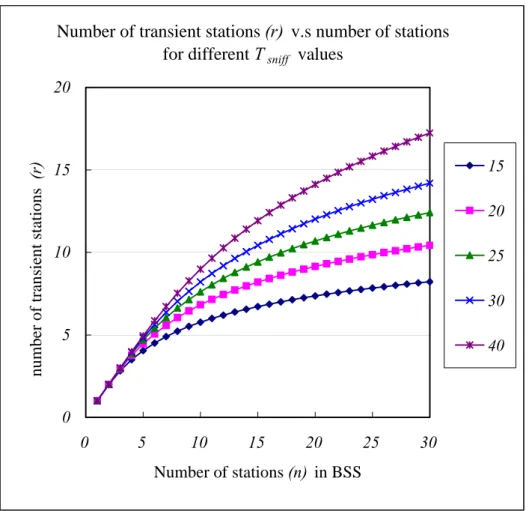
With equations (2)~(12) and parameters listed in Table 3.1 for an IEEE 802.11b wireless LAN, the relations of transient number of station(r) v.s. number of station(n) of various Tsniff values are demonstrated in Figure 3.7.

Parameters Values PLCP preamble & header 192.0 μs

MAC header 20.4 μs Slot time 20 μs

DIFS 50 μs

ACK 10.2 μs + PLCP preamble & header

CWmin 32

CWmax 1023

Maximal Packet payload 2312 bytes Channel bit rate 11 Mbps

Table 3.1 Parameters for IEEE 802.11b wireless LAN

Number of transient stations (r) v.s number of stations for different T_sniff values

0 5 10 15 20 0 5 10 15 20 25 30 Number of stations (n) in BSS number of transien t stations (r ) ₁₅ 20 25 30 40

Figure 3.7 Number of transient stations (r) v.s. number of stations (n) for different Tsniff values.

By reviewing equation (1), a station count (s) linearly depends on overlapped area (A’) and transient number of station(r) with respect to a Tsniff. Since it is desired

that a station count to indicates overlapped area (A’) rather than being disturbed by the imbalance of numbers of stations in different BSSs, an appropriate sniffing period

(Tsniff) should be set so that the number of transient stations (r) behaves insensitively

to variation of the number of stations (n).

Figure 3.7 shows the fact that a shorter sniffing period (Tsniff) responds to a

number of transient stations (r) less insensitive to variation of number of stations (n). However, as described in the previous section, a sniffing period should be long enough to make station counts big enough for a creditable selection. In this thesis, we recommend that in a BSS of fewer stations (such as n = 6), number of transient stations (r) should be 80 % of number of stations (n), i.e., r > 4.8 as n = 6. From the curves in Figure 3.7, a sniffing period Tsniff is eventually chosen as 20 ms because the

curve of Tsniff = 20 ms shows that its transient stations equal to 5 witht n = 6. As n =

24, the number of stations increases by 4 times, the number of transient stations (r) is approximately equal to 10, increased by only 2 times. The numerical result shows that the variation of number of stations in a BSS reflects only half of numbers of transient station by setting a sniffing period as 20 ms. Although there is no proper sniffing period to make number of transient stations independent of number of station, however, the effect brought by imbalance of number of stations has been significantly mitigated by 50%

3.3.3 Performance of Station Count Mechanism

E(s), the expected value of the station count with respect to a given Tsniff, is

approximately equal to r*A’/A as described in (1), while collisions within overlapped area, A’, is neglected. In this section, the collisions are taken into consideration for a

more accurate formula to estimate E(s).

The average number of stations lies in the overlapped coverage that is estimated by area proportion, so that n’ = n*A’/A. Let m’ denote the total frames sent by either one of n’ stations (no collision with any frame sent by one of n’ stations) in Tsniff, then

m’ is estimated in (13), where τ is given in (2) and m is given in (9)

n n m T T n m n av sniff n / ' ) 1 ( / ) 1 ( ' '= τ −τ '−1⋅ = ⋅ −τ '−1⋅ (13) Same as the process to estimate the number of transient stations, assuming that

n’ stations transmit m’ frames randomly and let μ denote the reformed station count, the number of stations that sends at least one of m’ frames in Tsniff. Thus, μ can be

derived using (14) below.

( ) (

( ) (

)

)

∑

∑

where, S(m,n) denotes the Stirling number of the second kind that is defined in (11), and P(n,k) denotes permutation number that is defined in (12)

Note that m’ in (13) may not be an integer and m’ in (14) is restricted to an integer. Interpolation is used for numerical approach below.

Let Si denote the random variable of station count in a sniffing period Tsniff for ith

channel. It is reasonably assumed that i Si features Poisson distribution.

ii μi,derived in (14), an estimation of reformed station count for ith channel,

should be the average of random variable Si, i.e., μi = E(si).

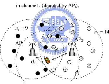
The scenario to display the performance of station count mechanism is illustrated in Figure 3.8. It assumes that a mobile node with discrete scan scheme roams in the overlapped coverage of two next-AP candidates. The current AP is not shown in

Figure 3.8, for its location will be irrelevant to performance of the station count mechanism. The mobile node selects one of two next-AP candidates, AP1 and AP2,

according to their station counts derived in the last two sniffing periods of the discrete scan. Let h denote the hit ratio, the probability that the mobile node selects the nearest AP with the indication of larger station count as its next AP. Therefore, the mathematical definition for h in the case of two candidates is given in (15).

) | ( 2 1 ) | (s₁ s₂ d₁ d₂ p s₁ s₂ d₁ d₂ p h= > < + = < (15)

where,p(…|…) denotes the conditioned probability.

si denotes the station count in Tsniff of ith channel.

di denotes the distance between the mobile node and the AP

in channel i (denoted by APi).

Figure 3.8 Scenario for performance estimation.

The average station count in each channel, μ1 and μ2, can be estimated by (14)

with given n1, n2, d1, d2, Tsniff as wells as parameters for DCF wireless environment

(listed in Table 3.1). Since S1 and S2 are in Poisson distribution of mean values E(s1)

= μ1 and E(s2) = μ2, the hit ratio h, defined in (15) is estimated by,

)] ( 2 1 ) ( [ ) ( 2 1 2 1 k p s k p s k s p h k = + < ⋅ = =

∑

] ) ! 2 ! ( ! [ 1 0 2 2 1 1 ) ( _{1 2}

∑

∑

Hit ratios are demonstrated for the conditions that the mobile node locates at the place

d1 = 0.5R and d2 varies from 0.5R to 1.2R, where R denotes the radius of coverage of

BSSs and the mobile node. Tsniff is set as 20 ms. In the first case, it demonstrates how

the distances between the mobile node and APs affect the hit ratio by setting the same number of stations in BSSs to ignore effects of the imbalance of numbers of stations in BSSs. In Figure 3.9, the curves are given for hit ratios (h) with respect to various distances from AP2 (d2) in cases of n1 = n2 = 6, 12, 18 and 24.

Hit ratios for balanced numbr of stations

d1=0.5R, d2=0.5R~1.2R 0.5 0.6 0.7 0.8 0.9 0.5 0.6 0.7 0.8 0.9 1 1.1 1.2 d2 / R Hit ratio n1=n2=6 n1=n2=12 n1=n2=18 n1=n2=24

Figure 3.9 Hit ratios v.s. distances in balanced number of stations.

Figure 3.9 shows that the hit ratios increase almost linearly with the increase of distance between the mobile node and the competing AP (d2), while the distance from

the mobile node to the selected AP (d1) is set fixed and the effect of imbalanced

number of stations are ignored, i.e., n1 = n2. From observation of Figure 3.9, it

independent to the hit ratios.

In the second case, we investigate the affect of imbalanced number of stations on the hit ratios. The mobile node keeps its location at the place d1 = 0.5R and d2 = 0.9R.

Four cases of variation of number of stations in BSS1, n1 = 6, 8, 10 and 12 are

individually input. For each case, the number of stations in BSS2, n2, varies from 0.6

to 2 times of n1 and the corresponding hit ratios are computed and presented in curves,

as shown in Figure 3.10.

Hit ratios v.s. imbalance of number of stations (n₂/n₁) handoff at d₁=0.5R, d₂=0.9R 0.5 0.6 0.7 0.8 0.9 0.6 0.8 1 1.2 1.4 1.6 1.8 2 n2/n1 Hit ratio n1=6 n1=8 n1=10 n1=12

Figure 3.10 Variation of hit ratios with imbalance of number of stations.

Observe the curves in Figure 3.9, the imbalance of number of stations do affect the hit ratios. In the neutral number of stations, i.e., n2 = n1, the hit ratios for all of the

four cases are about 0.68. With the increase of imbalance, i.e., increasing n2 / n1, the

hit ratios decrease with moderate slopes. As to the most imbalanced number of stations, i.e., case of n2 = 2n1, the hit ratios drop to about 0.55~0.6. The hit ratio

decreases by less than 20% due to the number of stations of competing BSS increases up to double. In addition, it is more sensitive to the disturbance of imbalance in

number of stations in case of fewer stations in the selected BSS (BBS1). In Figure

3.10, in the case that most of stations are in selected BSS (i.e., n1 = 12), the hit ratio

drops to about 10% (from 0.68 to 0.6) with the increase of imbalance (n2 / n1) from

1.0 to 2.0. On the other hand, the hit ratio drops to about 20% (from 0.68 to 0.55) in case that there are fewest stations in the selected BSS (n1 = 6).

3.3.4 Select Best Next AP Instead of the Nearest AP

The traditional handoff scheme that determines the next AP to handoff to by the RSS (receive signal strength) received from the responding AP in the probe phase of a layer-2 handoff. The strongest RSS is recognized as an indicator of the nearest AP, because shorter distance is subject to stronger signal strength. Same as RSS, the mechanisms presented in section 3.3.1 help a roaming node select the nearest AP by the link-layer information obtained in discrete scans. However, the nearest AP may not be the best next AP to handoff to. The available bandwidth that the next BSS can offer is one of the most concerned items especially for a mobile node in real time application, such as a WiFi VoIP connection. Besides, an AP that the mobile node is approaching to may be a better selection of the next AP than those from which the mobile node is moving away, even the latter ones are detected with stronger RSS.

Discrete scan schemes may be used to detect characteristics of a BSS by the collection of frames transmitted in a BSS in advance to a handoff. With information from sniffed frames, a mobile node may select the best next AP rather than the possible nearest AP with the indication of RSS in a traditional handoff scheme.

The available bandwidth and access delay of a BSS can be detected by the average NAV values in the frames collected in discrete scans. The relations between

the NAV values and available bandwidth as well as access delay in a BSS are inferred to be linearly dependent in [11] with both mathematical analysis and simulation. A mobile node with discrete scan will be able to estimate the available bandwidths and access delays of the next-BSS candidates by NAVs collected in its sniffing periods and determine the best next AP when a handoff is triggered.

Furthermore, the trends of station counts along certain sniffing periods for a BSS may be used to indicate whether the sniffing node is approaching to an AP or not. For the AP that a mobile node is approaching to, the station counts shall be in an increasing trend because the mobile node can listen to more stations when it is closing to the AP. To select an approaching AP rather than the nearest AP may alleviate the frequent handoffs in the hot spot where the cell of a BSS may be relatively small.

The attributes that assist a mobile node to determine its next AP in handoffs may be integrated as an objective function with appropriate weights assigned to all of the indicators. With combinational considerations on receive signal strength, distances, approaches, as well as available bandwidth, the objective function for a mobile node to evaluate ith BSS can be written as,

i i

i i

i w RSS w STA count w STA count w NAV

F = ₁( ) + ₂( _ ) + ₃(Δ _ ) + ₄( ) (17)

3.4 Impact on Service QoS

The most concerns on the discrete scan schemes may attribute to its impact on the service QoS in a pre-handoff period, since part of service time is taken out to sniff on other channels. During the sniffing periods, the service of working channel will be interrupted and this causes a certain level of access delay. Furthermore, because of absence from working channel, the frames that the current AP sends to the mobile

node during a sniffing period will be lost. However, as described in chapter 1, the applications that require seamless handoffs are mostly of relative low bit rate as compared with that a wireless NIC can offer. Therefore, with proper design, a mobile node may use a large portion of idle time of wireless NIC for discrete scan; thus, to minimize the impacts caused by discrete scan. In this section, a VoIP connection which runs with bidirectional 64 kbps constant bit rate in an IEEE 802.11b wireless LAN of 11Mbps are taken as an example for the discussion on the impact on service QoS brought by discrete scan scheme.

Besides a sniffing period of 20 ms, the channel switch time of a wireless NIC contributes to disruption of service from working channel as a major part. In this thesis, the channel switch time is assumed as 5 ms as in [1]. To complete a sniffing period in discrete scan scheme, it needs to do twice for switching channels, one for leaving from the working channel and the other for returning back. Therefore, it brings an absence period of at least 30 ms from the working channel to execute once of discrete scan.

A disruption of 50 ms may be the upper bound for a seamless handoff to tolerate. The principle of the discrete scan is to decompose time for the probe phase of a layer-2 handoff into a pre-handoff period, such that no more than 50 ms disruptions are induced during pre-handoff and handoff procedures.

Nowadays, the QoS issue for real time applications in IEEE 802.11 wireless LAN is still widely discussed. In most of infrastructure wireless LAN environment, downlink traffics from AP to all the stations is much heavier than the uplink traffic from a single station to the AP. However, the transmission opportunity of AP is same as that of a single station, thus the downlink flow shares the bandwidth with those uplink flows from all stations. In other words, the shared bandwidth of the downlink transmission from AP to arbitrary one of stations will be only 1/n of the bandwidth of

the uplink transmission to AP, where n denotes number of stations in a BSS. Because of the asymmetric nature between uplink and downlink transmission, a real time application with symmetric bidirectional transmission may suffer from severely degraded QoS of downlink flow when the number of stations in a BSS increases.

To address the QoS problems caused by asymmetric transmission opportunity for a specific station with symmetric bidirectional traffics, piggyback schemes [12] in IEEE 802.11 standard suppose to forward the downlink traffic as an attachment to a positive ACK frames from AP to stations. With piggyback schemes, the QoS issue of asymmetric transmission opportunity is therefore eliminated. The QoS provisioning to symmetric bidirectional service then is considered as the QoS to the uplink flow of the concerned station.

Total disruption < 50 ms STA in Power Save Mode STA in Normal Mode

awake + data PSM + data ACK + d ata ACK + d ata awake + data PSM + data ACK + d ata ACK + d ata Division B: Maximal 10 ms Division A: Maximal 10 ms 30 ms Sniffing node AP Time Working periods Switching periods Sniffing periods

Figure 3.11 Total disruptions induced by a discrete scan.

As illustrated in Figure 3.11, the total disruption caused by discrete scans should be computed from the transmission of the last frames before wireless NIC switches to a sniffing channel until the transmission of the first frame after wireless NIC returns