Structure and orientation of the moving vortex lattice in clean type-II superconductors
Dingping Li,1,3Andrey M. Malkin,2,3and Baruch Rosenstein3,41Department of Physics, Peking University, Beijing 100871, China
2Institute of Applied Physics, Russian Academy of Science, Nizhnii Novgorod 603600, Russia
3National Center for Theoretical Sciences and Electrophysics Department, National Chiao Tung University, Hsinchu 30050, Taiwan, Republic of China
4Department of Condensed Matter Physics, Weizmann Institute of Science, Rehovot 76100, Israel
(Received 13 February 2004; revised manuscript received 30 July 2004; published 30 December 2004)
The dynamics of the moving vortex lattice is considered in the framework of the time-dependent Ginzburg-Landau equation neglecting the effects of pinning. At high flux velocities the pinning dominated dynamics is expected to crossover into the interactions dominated dynamics for very clean materials recently studied experimentally. The stationary lattice structure and orientation depend on the flux flow velocity. For relatively velocities V⬍Vc=
冑
8B/⌽0/␥, where ␥ is the inverse diffusion constant in the time-dependent Ginzburg-Landau equation, and the vortex lattice has a different orientation than for V⬎Vc. The two orientations can be desribed as motion “in channels” and motion of “lines of vortices perpendicular to the direction of motion.” Although we start from the lowest Landau level approximation, corrections to conductivity and the vortex lattice energy dissipation from higher Landau levels are systematically calculated and compared to a recent experiment.DOI: 10.1103/PhysRevB.70.214529 PACS number(s): 74.40.⫹k, 74.25.Ha, 74.25.Dw
I. INTRODUCTION
The static Abrikosov flux lattice has been experimentally observed since the 1960s by a great variety of techniques and lateral correlations have been clearly observed recently up to tens of thousands of lattice spacings.1 The remarkable ad-vances in decoration, small-angle neutron scattering, and muon spin rotation techniques allowed a recently direct glimpse into the structure of the moving Abrikosov vortex systems.2–5It shows that at small flux flow velocities vortices move in channels as predicted in Ref. 7. When the flux flow velocity increases beyond the one corresponding to the criti-cal current, one observes a relatively well correlated hexago-nal lattice. The channels and the plastic flow at relatively low velocities are explained by the influence of pinning on the basis of theoretical arguments8 and confirmed by numerous simulations.8–12At high velocity of the moving lattice (cor-responding to the high electric field), the influence of disor-der is expected to diminish and a “moving Bragg glass” appears.8,13 Indeed Bragg peaks roughly at positions of the hexagonal lattice were observed5recently.
Since the theoretical prediction of the moving Bragg glass exhibiting the transverse peak effect,13much effort has been put into the simulation of the high driving force phase of the moving vortex system.10–12In particular it was found10 that as the driving force increases(or disorder decreases) the vor-tex lattice suddenly changes orientation for a period of time and then returns to a “regular” drift mode. The main empha-sis in these studies mentioned above is still the effects of pinning on the moving lattice.
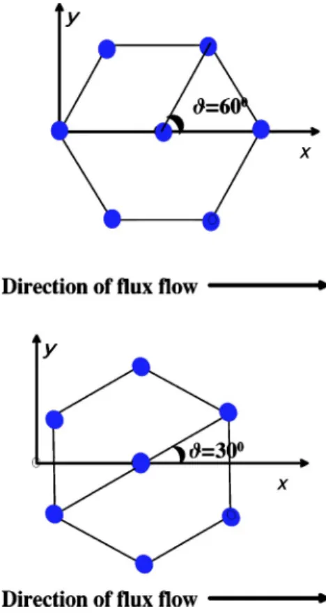
Experiments at a low (below 100 G) magnetic field and slow flux moving velocity(of orderm / s) showed that the orientation of the moving vortex lattice is tied to the direc-tion of modirec-tion, namely, when a nearly hexagonal lattice is observed, one always observes the orientation depicted in Fig. 1(a), never the “rotated” one of Fig. 1(b).4 Here the
effect of pinning cannot be ignored and plays an important role in the orientation of the vortex lattice. However, the most recent small-angle neutron scattering and muon spin
FIG. 1. Two possible orientations of the(approximately) hex-agonal vortex lattice.(a) The direction of the flux lines is the same as the nearest neighbors lattice orientation.(b) The direction of the flux lines is perpendicular to the nearest neighbors lattice orientation.
rotation experiment can probe the moving lattice at much higher velocities of order cm/s or even higher. The results about the orientation of the moving lattice obtained in Ref. 5 seem to be different from the case at a low magnetic field and slow flux moving velocity.
The effect of pinning is expected to be smaller at higher velocities. Alternatively one can ask what happens in very clean materials. A recent experiment in Pn- In seems to be-long to this category.5 As the pinning influence diminishes with increasing flux velocity, it is natural to ask what would happen in the limit of the highest possible flux velocity(of course, eventually the electric field destroys superconductiv-ity, so that the mathematical limit of the infinite driving force is unphysical) disregarding pinning altogether.
The question of the orientation of the vortex lattice usu-ally does not arise in the static case. Without an external electric field singling out a particular direction one has a complete degeneracy of possible orientations of the hexago-nal vortex lattice. This is not surprising for a sufficiently symmetric material (like NbSe2 frequently used in experi-ments belongs to this category): the rotational symmetry en-sures that the free energy is independent of the hexagonal lattice orientation. The rotational symmetry is broken by the motion of fluxons as was confirmed experimentally.4,6 Natu-rally one could ask whether the particular lattice orientation observed for example in Ref. 4 is necessarily tied to pinning or might appear in clean superconductors as well. Further-more, the lattice also can be deformed though the deforma-tion apparently is very small[see Figs. 1(c) and 1(d) in Ref. 4]. Is there a deformation even before pinning centers disor-der the lattice?
It would be difficult to address the question of the moving vortex lattice structure using phenomenological models like the elastic medium13(in which individual vortices are simply not “seen”) or approximating vortices in the London ap-proximation by interacting lines or points ri in two
dimen-sions (2D).12 To give an example of the problems in the London limit, let us consider equations of motion for vorti-ces. The driving force F is the Lorentz force and the dynam-ics is assumed overdamped:
dri
dt = −
兺
j⫽i U共ri− rj兲 + F, 共1兲where U共ri− rj兲 is the intervortex repulsive potential. The
solution of these equations in the absence of pinning is ob-vious: the “boosted” hexagonal lattice of any orientation ir-respective of the direction of F. Thus the orientation of the lattice depends solely on initial conditions, at least in the clean case. Therefore the approximations made in the above phenomenological approaches are too strong.
In this paper we use the time-dependent Ginzburg-Landau
(TDGL) model to study the vortex motion and structure. The
TDGL approach has been remarkably successful in describ-ing various thermodynamical and transport properties.14 Progress in obtaining the theoretical results from the model can be achieved only when certain additional assumptions are made. One of the often made additional assumption is that only the lowest Landau level(LLL) significantly
con-tributes to physical quantities of interest. The LLL approxi-mation is valid for H⬎Hc2共T兲/13 in the static limit.15
Al-though most of the experiments concerning a moving lattice were performed at a field far below the static Hc2共T兲, it has
been shown a long time ago16,17that in the presence of elec-tric field E the effective Hc2共T,E兲=Hc2共T兲−␥2V2⌽0/共8兲 where V = cE / B is the velocity of fluxons and␥is the inverse diffusion constant setting the time scale in the TDGL ap-proach. This field Hc2共T,E兲 could be much smaller at not
very small fluxon velocities(electric field suppresses super-conductivity even more effectively than the magnetic field). Therefore effectively one can move into the region of valid-ity of the LLL approximation at sufficiently large currents. Moreover, one expects that, even beyond the region of va-lidity of the LLL approximation, physics is qualitatively the same.
We solve TDGL equations for a moving vortex solid with-out disorder and find the vortex structure to which the mov-ing lattice relaxes irrespective of initial conditions.16–18 It turns out that the preferred lattice is rhombic. The distortion is velocity dependent. Remarkably the orientation is the same as in Fig. 1(a); namely, it agrees with experiments only at velocities exceeding the critical one(of order of cm/s for superconducting type II low Tcmetals). Below it the
orien-tation is rotated by 30°.
The paper is organized as follows. The model is de-scribed, symmetries analyzed, and the perturbative mean field solution developed in Sec. II. The general formalism is developed to treat the non-Hermitian part of the equation. The shape and the orientation of the vortex lattice and the reorientation transition are described in Sec. III. Then in Sec. IV we calculate corrections due to higher Landau levels and derive a general expression for conductivity. It is compared with a recent experiment. Section V is a summary.
II. MODEL AND ITS PERTURBATIVE FLUX FLOW SOLUTION
A. Time-dependent GL model
Our starting point is the TDGL equation,19
ប2␥ 2mab
冉
t+ ie* ប ⌽冊
= − ␦ ␦*F. 共2兲 The static GL free energy isF =
冕
d3x冉
ប 2 2mab冏
冉
ⵜជ +ie* បcAជ冊
冏
2 + ប 2 2mc 兩z兩2−␣共Tc− T兲 ⫻兩兩2+b⬘
2兩兩 4冊
, 共3兲where␣ and b
⬘
are phenomenological parameters,␥ is the inverse diffusion constant which controls the scale of dy-namical processes via dissipation. As usual the magnetic in-duction is Bជ=ⵜជÃAជ and electric field Eជ= −ⵜជ⌽−共/t兲Aជ. It should be supplemented by Ampere’s law17,18ⵜជ Ã Bជ=nEជ+ Jជs, 共4兲
where the first term is the contribution of the normal liquid in the framework of the two liquid model and the second term is the supercurrent J ជs= −iបe* 2m *
冉
ⵜជ + ie* បcAជ冊
+ c.c. 共5兲Tensorn is the normal state conductivity. We assume that
the coefficient of the covariant time derivative term␥in Eq.
(2) is real although a small imaginary (Hall) part is always
present.18The general case will be discussed in Sec. V. We make several approximations(identical to those made in Ref. 20 and major parts of Ref. 17) so that the problem becomes manageable. The physical conditions allowing those approximations are the following. Temperatures and magnetic fields are close “enough” to Hc2共T兲. Under this
assumption the order parameteris suppressed compared to its Meissner value. In this paper we will also assume strongly type II superconductivity=/Ⰷ1 [2=ប2/共2m
ab␣Tc兲, 2
= c2m * b
⬘
/ 4e*2␣Tc]. The magnetic field is veryhomoge-neous since the vortices overlap. The characteristic length describing the inhomogeneity of the electric field was iden-tified in Ref. 17:2=共4
n/␥兲2and since typicallyn⯝␥,
thus Ⰷ and the electric field is assumed homogeneous. Therefore the Maxwell type equations for the electromag-netic field are not considered. The time-independent vector potential will be taken in Landau gauge Aជ=共By,0,0兲 and describes a nonfluctuating magnetic field in the direction −zˆ. The scalar potential is also independent of time A0= Ey and describes the electric field oriented along the negative y axis. The vortices are therefore moving along the x direction. We neglect thermal fluctuations and disorder on the mesoscopic scale.
Throughout most of the paper we will use the following physical units. The unit of length is the coherence length, the unit of the magnetic field is Hc2=⌽0/ 22, =共c/e*兲
冑
mabb⬘
/ 4␣Tc, and the unit of energy(temperature) is Tc. In these units the magnetic field is denoted by b⬅B/Hc2. The asymmetry of masses between the z direction
and the x-y plane can be removed by rescaling coordi-nates and time: x→x /
冑
b, y→y /冑
b, z→z /冑
bmc/ mab,t→共␥2/ 2b兲t. The TDGL equations, after the order param-eter field is rescaled as well→
冑
2␣Tcb / b⬘
, are0 = L+兩兩2, 共6兲 L⬅ Dt− 1 2关Dx 2 +y2+z2兴 − a,
where a⬅共1−T/Tc/ 2b兲, v=共c␥E / 2B兲
冑
បc/e*B is scaledvortex velocity(in units of 2
冑
2B /⌽0/␥), and covariant de-rivatives are defined by Dx=/x − iy and Dt=/t + ivy.Sincez2commutes with L, the equations are invariant under the z translations, the z dependence of the solutions de-couples and is generally a plane wave. It is easy to see that the relevant solution does not break this symmetry and is therefore constant with respect to z. Consequently we con-sider the problem as a 2 + 1-dimensional one[note, however, that if the three-dimensional(3D) disorder or thermal
fluc-tuations are included one cannot ignore the z coordinate as the configuration of disorder can destroy the translational symmetry along the z direction].
B. Expansion of a nontrivial solution around dynamical phase transition point
The line in parameter space 共a,v兲, which separates the normal region in which the only solution is = 0 from the flux flow nontrivial solution region, has been found by Hu and Thompson.17We will construct a perturbative solution of the TDGL equations near the mixed state–normal phase tran-sition line analogous to the one in statics.21 The range of applicability and precision of the LLL approximation at large in statics was explored recently.15 The main difficulty in the dynamical case is that the linear part of the equation L is not Hermitian due to the dissipation term Dt.
A general idea of the expansion around a bifurcation point of a nonlinear equation is as follows. One looks for a set of eigenfunctions of the linear part of Eq.(6):
LNp=⌰NpNp. 共7兲 The operator L consists of two parts: the usual Hermitian Hamiltonian of a particle in magnetic field −12关Dx2+y2兴 and the anti-Hermitian covariant time derivative Dt. The
com-plete set of eigenfunctions with “quantum” numbers N and
px⬅p is
Np=
1
冑
2NN!⫻exp关i共px −t兲兴HN共y − p + iv兲 ⫻exp
冋
−1 2共y − p + iv兲 2册
, 共8兲 ⌰Np= − a + N + 1 2+ v2 2 − i共−vp兲,where HN are Hermitian polynomials. Unlike the usual case
of a Hermitian operator, eigenfunctions and eigenvalues of the Hermitian conjugate of the operator L†are different:
L†Np=⌰NpNp,
¯
Np=
1
冑
2NN!exp关− i共px −t兲兴HN共y − p + iv兲⫻exp
冋
−1 2共y − p + iv兲 2册
, 共9兲 ⌰¯ Np= − a + N + 1 2+ v2 2 + i共−vp兲.Note that¯ is not a complex conjugate of. The orthogo-nality relations in the dynamical case involve bothNpand
¯
冕
x,y,t ¯Np 共x,y,t兲N⬘p⬘⬘共x,y,t兲 =共2兲2␦NN⬘␦共p − p⬘
兲 ⫻␦共−⬘
兲, 共10兲 具¯Np共x,y,t兲Np共x,y,t兲典x,y,t= 1,
where the averaging over space and time is denoted by
具¯典x,y,t.
The bifurcation(in this case the dynamical transition) oc-curs when there exists a set of eigenfunctions of L
⬘
with zero eigenvalues⌰Np= 0: abif共v兲 = N +1 2+ v2 2 , 共11兲 =vp. 共12兲It is clear that solutions with N⬎0 are unstable as in the static case.19 Equation (11) with N=0 gives the phase tran-sition line of Ref. 17, while Eq.(12) selects the “zero mani-fold” in the space of functions. We define the “distance” from the transition line
ah共v兲 ⬅ a − abif共v兲 = a −1
2−
v2
2 . 共13兲
When ah共v兲⬎0, the nonlinear TDGL equation,
L+兩兩2⬅ Lsh− ah共v兲+兩兩2= 0, 共14兲
Lsh= L + ah共v兲,
is solved perturbatively in ahwith a nonanalytic prefactor, as in the static case:
⌽ = 关ah共v兲兴1/2关⌽0+ ah⌽1+ ¯ 兴. 共15兲
To order关ah兴1/2, the equation linearizes
Lsh⌽0= 0. 共16兲 Therefore⌽0belongs to the “zero manifold” and thereby can be expanded, ⌽0=
兺
p cpN=0,p,=vp⬅兺
p cpp, 共17兲with coefficients cp determined by the next order equation.
As a result, since all thep共x,y,t兲 depend only on the
com-bination px −t = p共x−vt兲 rather than separately on x and t,
vortices move in the direction perpendicular to both the elec-tric and the magnetic field with constant velocityv. To order
关ah兴3/2, one obtains
Lsh⌽1=⌽0−⌽0兩⌽0兩2.
Multiplying this equation by¯pand integrating over共x,y,t兲
using the orthogonality relation, Eq. (10), one obtains the following infinite set of nonlinear algebraic equations:
兺
p1,p2,r cp1cp2cr *具¯ pr * p1p2典x,y,t= cp. 共18兲We will study the solution of this set in the next section.
III. SHAPE AND ORIENTATION OF THE MOVING LATTICE
A. Symmetry and energetics considerations
It is well known in the static case that there is a solution of GL equations for any lattice symmetry. The same is true in the dynamical case as well, but the symmetries should take into account the motion of vortices. We define the covariant derivatives in a matrix 2 + 1-dimensional form(a summation over repeated indices assumed),
A= bx, D=− iA, 共19兲 and the Landau gauge
共20兲
is used in our paper. All indices run over space= 1共x兲, 2共y兲, and 3共t兲. The electromagnetic translation operators satisfying
关Td, D兴=0 are
Td= eid·P= exp
冋
− i冉
1
2dbd+ xbd
冊
册
eid·p, 共21兲
where generators are P= −i共− ibx兲 (note a transpose in
the matrix b). Operators p= −i are usual(not “electro-magnetic”) translation operators. The following commutation relations:
关P, P兴 = i共b− b兲, 共22兲
can be verified. Thus we will have 关id1· P , id2· P兴 = −id1␣d2共b␣− b␣兲. Using the Haussdorf formula one checks that the electromagnetic translation operators obey
eid1·Peid2·P= eid2·Peid1·Pe关id1·P, id2·P兴.(See Fig. 2.) If d
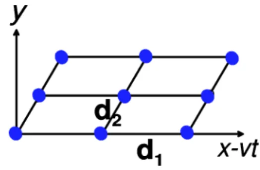
1 and d2 are the lattice vectors which preserve the symmetry of the system (when one translates the system by d1 or d2, the system will be unchanged), one shall require eid1·P = eid2·Pand it will lead to
FIG. 2. The flux lattice geometry: d共1兲, d共2兲are the translational symmetry vectors which determines the primitive cell of the flux lattice. The angle between these two vectors is.
eid1·Peid2·P= eid2·Peid1·Pe关id1·P, id2·P兴= e关id1·P, id2·P兴=. Therefore we should demand
关id1· P, id2· P兴 = i2⫻ integer.
This requirement is satisfied by the following basic transla-tion symmetry vectors:
d共1兲= a⌬
冉
1 2,0,− 1 2v冊
, d共2兲= a⌬冉
r 2,r⬘
,− r 2v冊
, 共23兲 d共0兲=共v,0,1兲.Here a⌬is the lattice spacing along the direction of motion, is arbitrary (a continuous translational symmetry). The flux quantization(one flux quantum per unit cell assumed) deter-mines r
⬘
: r⬘
a⌬2= 2. The d共1兲 translation symmetry leads to the discrete parameterp =2 a⌬l⬅ gl,
in Eq. (17), and the set of equations, Eq. (18), will take a form cn=
冑
1 2g 2兺
l1,l2 cl1+ncl2+ncl1+l2+n * ⫻exp再
−1 2关共gl1+ iv兲 2+共gl 2+ iv兲 2− v2兴冎
. 共24兲 It can be solved as in the static case by an Ansatzcl=
冑
g
冑
A共v兲e−irl共l+1兲, with the Abrikosov function
A共v兲 = g
冑
2l1,l2兺
⫻exp兵2irl1l2其 ⫻exp再
− 1 2关共gl1+ iv兲 2+共gl 2+ iv兲2−v2兴冎
. 共25兲 Consequently, ⌽0共x,y,z兲 = 1冑
A共v兲 共x,y兲, 共26兲 where 共x,y兲 ⬅冑
冑
g 兺
l exp兵il关g共x − vt兲 −r共l + 1兲兴其 ⫻exp冋
−1 2共y − gl − iv兲 2册
共27兲 is normalized by具兩兩2典x,y= 1.In the static case a solution which has minimal free en-ergy is physically realized. The free enen-ergy is proportional to −关ah共0兲兴2/关2A共0兲兴 which therefore should be minimized.
This means that one should minimize A共0兲. The minimal
A共0兲=1.16 is obtained for the hexagonal lattice. Similar
reasoning cannot be applied to the moving lattice solution of the TDGL equation since the friction force is nonconserva-tive. Under these circumstances Ketterson and Song22 calcu-lated the work made by the friction force:
S⬅ d
dtS = 2␥具兩Dt兩
2典
x,y. 共28兲
The preferred lattice structure in the steady state corresponds to a state with largest S˙. For the lattice solution of the TDGL equation one obtains to leading order in␣h,
S˙⬀g兩␣h共v兲兩 A共v兲
冓
冏
兺
l冉
t+ ivy冊
exp兵il关g共x − vt兲 −r共l + 1兲兴其exp冋
−1 2共y − gl − iv兲 2册
冏
2冔
x,y =v 2兩␣ h共v兲兩 2A共v兲 ev2. 共29兲We therefore shall minimizeAas function of r and a⌬. This
is consistent with the static case.
B. The stationary orientation of the flux lattice. The reorientation transition at high flux flow velocity
We found that the minimum of A共v兲 always appears
when r = 1 / 2, namely for rhombic lattices. Therefore from now on we consider these lattices only. As a function of an angle of the rhombic lattice tan= 4/ a⌬2 (see Fig. 1 for a definition of) it generally has two minima; see Fig. 3. In the static case the two minima are degenerate with = 60°, 30° corresponding to perpendicular orientations of the hex-agonal lattice, while for nonzero velocity the degeneracy is lifted. Note that originally16,17it was assumed that the lattice is hexagonal also in the dynamical case. Generally the shape is not strongly distorted for physically realizable velocities. For velocities smaller thanvc= 0.95 angleclose to 60°[the
orientation of Fig. 1(b)] is preferred over the one close to 30°
[the orientation of Fig. 1(a)]; see Fig. 3(c). The dependence
of the angleon velocity can be very well fitted in the whole rangev⬍0.5 by
= 30 − 0.4v − 24v2. 共30兲 The Abrikosov function also depends on velocity increasing according to
A共v兲 =A共0兲共1 + 1.25v2兲, 共31兲
whereA共0兲=1.1596 is the static value for a hexagonal
lat-tice. As the critical velocity is approached the two minima coincide; see Fig. 3(b). Beyond that point the preferred struc-ture is just the opposite; Fig. 3(a). The transition is first order and the coexistence region should exist.
We now make a few comments about the orientation of the lattice. The reader might have noticed that the orientation
of the lattice is not completely arbitrary since the direction of the vector d1 coincides with the direction of the vortex mo-tion. The most generalA共v兲 is given by Eq. (25) with
arbi-trary r. We minimized numerically the Abrikosovfunction and found that the solution with the largest dissipation is always of the more symmetric type r = 1 / 2. One can argue that despite the fact that the electric field breaks the continu-ous rotational symmetry, it still preserves a discrete transfor-mation y→−y, →*. The solution r = 1 / 2 preserves this discrete symmetry. This symmetry is unlikely to be sponta-neously broken. Indeed the symmetry was observed in the experiments(for example, in Ref. 4).
IV. NONLINEAR CONDUCTIVITY AND BREAKDOWN OF THE LLL SCALING IN TRANSPORT
In this section we first calculate the leading higher Landau level corrections to the solution of the TDGL equation, Eq.
(6). Then we use it to derive the correction to the LLL
scal-ing of conductivity.18,20,23
A. Higher orders in ahcorrection to the moving lattice
solution
Using the same symmetry arguments as for the leading order, the second term in Eq.(15) can be expanded as
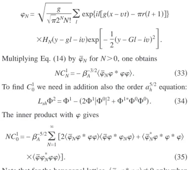
⌽1=
兺
N=0 CN1N, 共32兲 N=冑
g冑
2NN!兺
l exp兵il关g共x − vt兲 −r共l + 1兲兴其 ⫻HN共y − gl − iv兲exp冋
− 1 2共y − Gl − iv兲 2册
. Multiplying Eq.(14) by¯Nfor N⬎0, one obtainsNCN1 = −A−3/2具¯N*典. 共33兲 To find C01we need in addition also the order ah5/2equation:
Lsh⌽2=⌽1−共2⌽1兩⌽0兩2+⌽1ⴱ⌽0⌽0兲. 共34兲
The inner product withgives
NC0 1 = −A −5/2
兺
N=1 ⬁ 关2具¯N*典具¯*N典 + 具¯N * **典 ⫻具¯N*典兴. 共35兲Note that for the hexagonal lattice,具¯N*典⫽0 only when
N = 6j, where j is an integer. This is due to hexagonal
sym-metry of the vortex lattice.21 In statics 
N=具¯N*典
de-creases very fast with j: 6= −0.2787, 12= 0.0249.15 Be-cause of this the coefficient of the next to leading order is very small(also an additional factor of 6 in the denominator helps the convergency).
B. The LLL scaling in nonlinear conductivity
In the flux flow regime, in addition to the normal state conductivity, there is a large contribution from the Cooper pairs represented by the order parameter field. It was noted in Refs. 18, 20, and 23 that the LLL contribution to nonlinear conductivity, = − iបe * 2mE*
冉
ⵜជ + ie* បcAជ冊
, 共36兲is proportional to the superfluid density. The scaled dimen-sionless conductivity is defined asscaled⬅共42/ c2␥兲and
scaledin the LLL approximation is
LLL= i 2v具⌿LLL * y⌿LLL−⌿LLLy⌿LLL * 典 = 具兩⌿ LLL兩2典. 共37兲
The last equality is due to the general property of the LLL functions; see Eq. (8). It follows the naive expectation of a “Drude”-like formula19 with 兩⌿
LLL兩2 playing a role of
“charge carriers” density(meaning here Cooper pairs). To leading order in ahusing the results of Sec. II one gets
LLL= iah共v兲 2A共v兲v 具*y−y*典 = ah共v兲 A共v兲 ev2, 共38兲 where ah共v兲=共1−tGL− b −v2兲/共2b兲. At finite v there is an
ex-ponential factor coming from the nonorthogonality of eigen-functions of a non-Hermitian operator and, in addition, simi-lar dependence inA and quadratic in ah. In the limitv→0
one recovers the Ohmic expression(see Ref. 18) returning to standard units,
FIG. 3. The dependence of the Abrikosov parameter on ori-entation and shape of the vortex lattice moving with scaled
veloci-tiesv = 0.5,0.95, 1.1. The angle is defined as an angle between the
direction of motion and a crystallographic axis in the direction of the symmetry transformation d2. The minimum favors the smaller angle close to 30° corresponding to the structure of Fig. 1(a) for v⬍vc, while the other local minimum corresponding to Fig. 1(b)
LLL共1兲 =0
1 − tGL− b
2bA共0兲 , 0⬅
c2␥
42, 共39兲 while the leading nonlinear(cubic) correction is, using Eq.
(31), LLL共3兲 =0 tGL+ b − 5 8bA共0兲 v2, 共40兲 wherev =共c␥E / 2B兲
冑
បc/e*B.C. Leading correction to the LLL scaling
Generally to all orders in ah one can write ⌿
=兺NCN共ah兲N, =0 i 2v
兺
NM CN*共ah兲CM共ah兲具N * yM−MyN *典 ⬅0兺
NM CN*共ah兲CM共ah兲NM. 共41兲For N⬎M and N−M even integer,
NM= −
冑
2N−MM! N! 共− v 2兲共N−M兲/2冋
v2LN−M+1M−1 共− 2v2兲 +M + 1 2 LM+1 N−M−1共− 2v2兲册
ev2, 共42兲where L共y兲 are Laguerre polynomials. This contribution is always sub-OhmicNM⬃vN−M at small v. If N − M is odd,
the contribution vanishes. The diagonal contributions are simpler,
NN=关LN−1
1 共− 2v2兲 + L
N
1共− 2v2兲兴ev2, 共43兲
and have an Ohmic part,
NN= 2N + 1.
The first term, proportional to Landau orbital number N, is responsible for the breaking of the naive Drude-like expec-tation that conductivity is proportional to 兩⌿兩2.19 One ob-serves that higher Landau levels contribute to conductivity more than to 兩⌿兩2. One can interpret this as an “increased charge movers density.”
Thus the Ohmic conductivity has two contributions, 共1兲= 0
兺
N 共2N + 1兲兩CN共ah兲兩2=1+2, 共44兲 1=0具兩⌿兩2典, 2= 20兺
N=1 N兩CN共ah兲兩2, 共45兲the first proportional to the superfluid density, while the sec-ond, the HLL part, is not and is of order ah3only. Substituting expressions for C0 from the previous section, we obtain for the Ohmic conductivity to order ah2,
1=0
冋
ah A + 3ah 2 A 3兺
N=1 N 2 N册
, 共46兲where all the quantities are taken in the limitv→0. The sum rapidly converges in the static (or low velocity) case:
兺N共N
2
/ N兲=0.0131.
D. Comparison with experiment
In Fig. 4 we compare the results with recent experiments at high currents(electric fields) of Ref. 24 on Nb in which vortex velocities are as high as 105cm/ s. We used the same values of the Ginzburg-Landau parameter = 9.4 and the inverse diffusion constant ␥= 1.17 s / cm2 to fit all three curves corresponding to magnetic fields H = 80 mT, 100 mT, and 120 mT for a “cold” sample with Tc= 8.6 K. We
used the measured (inset in Fig. 2 of Ref. 24) Hc2
⬅Tc兩关dHc2共T兲/dT兴兩T=Tc= 4.4 T. The temperature was T
= 7.8 K close enough to Tc so that the ah
2
correction was always below 10%. The value of parameter ␥ is in good agreement the measured normal state resistivity of 9.9⍀ cm. The results agree well with the flux flow Ohmic conductivity data at relatively low currents(still well above the critical current) exhibiting the 1/H behavior presented in Fig. 2 of Ref. 24.
One observes that the full expression(solid lines) is closer to the experiment at very high electric fields. Several curves for the magnetic field are given. The smallest is clearly off the LLL approach range.
V. CONCLUSION
To summarize, we have considered the dynamics of the vortex lattice, neglecting the effects of pinning. We studied the time-dependent Ginzburg-Landau equation in the lowest Landau level approximation. For the validity region of the LLL approximation, as in the static case, we require ah
=共1/2B兲关Hc2共T兲−B−共c2␥2⌽0E2/ 4B2兲兴Ⰶ6, the factor 6 FIG. 4. Current-voltage curves at high flux flow velocities. The data of Ref. 24 on Nb films at T = 7.8 K(symbols represent different magnetic fields) are compared with theory combining the linear
coming from cancellations of the higher Landau level effects due to hexagonal symmetry(even the hexagonal symmetry is approximate in the moving lattice). We systematically calcu-lated higher Landau level corrections to conductivity and the vortex lattice energy dissipation. The stationary lattice struc-ture depends on the flux flow velocity. While for small ve-locities V⬍2vc冑2B /⌽0/␥, the vc= 0.95 vortex lattice is
oriented as in Fig. 1(b), while beyond this velocity orients as in Fig. 1(a). We emphasize that in our calculation the pinning effect was disregarded. Of course, as was firmly established in numerous theoretical and experimental investigations, pin-ning significantly can modify the picture for low velocities. Pinning generally “prefers” the configuration of Fig. 1(a) and this is a possible reason why the experimental observed ori-entation is depicted as in Fig. 1(a). However one can expect that for higher velocities and very clean samples the pinning dominated dynamics crosses over into the interactions domi-nated dynamics considered in the present work. The high velocity of order cm/s is unlikely to be seen in decoration
experiments. However other techniques like SANS and muon spin rotation5 and possibly Lorentz microscopy25 are able to detect the lattice structure even at such relatively high velocities. At very high velocities the results for nonlinear conductivity agree with recent experiments24.
ACKNOWLEDGMENTS
We are especially grateful to F. P. Lin for fitting the con-ductivity data. We are grateful to E. Andrei, A. Knigavko, T. J. Yang, A. Shaulov, Y. Yeshurun for a discussion, and E. M. Forgan for a discussion and sending results prior to publica-tion. The work of A.M. was supported by the graduate stu-dents program of NCTS. The work of B.R. was supported by the NSC of the R.O.C., NSC No. 932112M009024 and the hospitality of Peking University. The work of D.L. was sup-ported by the Ministry of Science and Technology of China
(Grant No. G1999064602) and the National Natural Science
Foundation of China(Grant No. 10274030).
1P. Kim, Z. Yao, C. A. Bolle, and C. M. Lieber, Phys. Rev. B 60, R12589(1999).
2U. Yaron et al., Phys. Rev. Lett. 73, 2748(1994).
3M. Marchevsky, J. Aarts, P. Kes, and M. Indenbom, Phys. Rev. Lett. 78, 531(1997).
4F. Pardo, F. de la Cruz, P. L. Gammel, E. Bucher, and D. J. Bishop, Nature(London) 396, 348 (1998).
5D. Charalambous, P. G. Kealey, E. M. Forgan, T. M. Riseman, M. W. Long, C. Goupil, R. Khasanov, D. Fort, P. J. C. King, S. L. Lee, and F. Ogrin, Phys. Rev. B 66, 054506(2002).
6E. Andrei(private communication).
7L. Balents, M. C. Marchetti, and L. Radzihovsky, Phys. Rev. B
57, 7705(1998).
8A. E. Koshelev and V. M. Vinokur, Phys. Rev. Lett. 73, 3580
(1994).
9K. Moon, R. T. Scalettar, and G. T. Zimanyi, Phys. Rev. Lett. 77, 2778(1996).
10C. J. Olson and C. Rechhardt, Phys. Rev. B 61, R3811(2000). 11H. Fangohr, S. J. Cox, and P. A. J. de Groot, Phys. Rev. B 64,
064505(2001).
12M. Chandran, R. T. Scalettar, and G. T. Zimanyi, Phys. Rev. B
67, 052507(2003).
13T. Giamarchi and P. Le Doussal, Phys. Rev. Lett. 76, 3408
(1996); Phys. Rev. B 57, 11356 (1998).
14E. H. Brandt, Rep. Prog. Phys. 58, 1465(1995). 15D. Li and B. Rosenstein, Phys. Rev. B 60, 9704(1999). 16C. Caroli and K. Maki, Phys. Rev. 164, 591(1967).
17R. S. Thompson and C.-R. Hu, Phys. Rev. Lett. 27, 1352(1971). 18R. J. Troy and A. T. Dorsey, Phys. Rev. B 47, 2715(1993). 19M. Tinkham, Introduction to Superconductivity (McGraw-Hill,
New York, 1996).
20T. Blum and M. A. Moore, Phys. Rev. B 56, 372(1997). 21G. Lasher, Phys. Rev. 140, A523(1965).
22J. B. Ketterson and S. N. Song, Superconductivity (Cambridge University Press, Cambridge, 1999), Chap. 21.
23A. Ikeda, T. Ohmi, and T. Tsuneto, J. Phys. Soc. Jpn. 59, 1740
(1990); 61, 254 (1992); A. Ikeda, ibid. 64, 1683 (1994); 64,
3925(1995).
24C. Villard, C. Peroz, and A. Sulpice, J. Low Temp. Phys. 131, 516(2003); C. Peroz et al., Physica C 369, 222 (2002). 25A. Tonomura, J. Low Temp. Phys. 131, 941(2003).