Counting Spanning Trees
∗Bang Ye Wu Kun-Mao Chao
1
Counting Spanning Trees
This book provides a comprehensive introduction to the modern study of spanning trees. A span-ning tree for a graph G is a subgraph of G that is a tree and contains all the vertices of G. There are many situations in which good spanning trees must be found. Whenever one wants to find a simple, cheap, yet efficient way to connect a set of terminals, be they computers, telephones, factories, or cities, a solution is normally one kind of spanning trees. Spanning trees prove important for several reasons:
1. They create a sparse subgraph that reflects a lot about the original graph. 2. They play an important role in designing efficient routing algorithms.
3. Some computationally hard problems, such as the Steiner tree problem and the traveling salesperson problem, can be solved approximately by using spanning trees.
4. They have wide applications in many areas, such as network design, bioinformatics, etc. Throughout this book, we use n to denote the number of vertices of the input graph, and m the number of edges of the input graph. Let us start with the problem of counting the number of spanning trees. Let Kn denote a complete graph with n vertices. How many spanning trees are there in the complete graph Kn? Before answering this question, consider the following simpler question. How many trees are there spanning all the vertices in Figure 1?
1 2
3 4
Figure 1: A four-vertex complete graph K4.
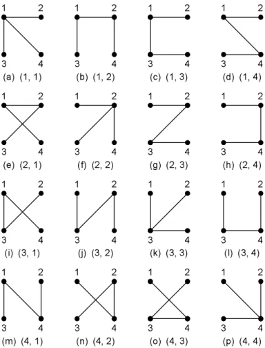
The answer is 16. Figure 2 gives all 16 spanning trees of the four-vertex complete graph in Figure 1. Each spanning tree is associated with a two-number sequence, called a Pr¨ufer sequence, which will be explained later.
Back in 1889, Cayley devised the well-known formula nn−2 for the number of spanning trees in the complete graph Kn [1]. There are numerous proofs of this elegant formula. The first explicit
∗An excerpt from the book “Spanning Trees and Optimization Problems,” by Bang Ye Wu and Kun-Mao Chao
(e) (2, 1)
1
2
3
4
(d) (1, 4)
1
2
3
4
(c) (1, 3)
1
2
3
4
(b) (1, 2)
1
2
3
4
(f) (2, 2)
1
2
3
4
(g) (2, 3)
1
2
3
4
(h) (2, 4)
1
2
3
4
(a) (1, 1)
1
2
3
4
(p) (4, 4)
1
2
3
4
(o) (4, 3)
1
2
3
4
(n) (4, 2)
1
2
3
4
(m) (4, 1)
1
2
3
4
(l) (3, 4)
1
2
3
4
(k) (3, 3)
1
2
3
4
(j) (3, 2)
1
2
3
4
(i) (3, 1)
1
2
3
4
Figure 2: All 16 spanning trees of K4.
combinatorial proof of Cayley’s formula is due to Pr¨ufer [2]. The idea of Pr¨ufer’s proof is to find a one-to-one correspondence (bijection) between the set of spanning trees of Kn, and the set of Pr¨ufer sequences of length n − 2, which is defined in Definition 1.
Definition 1: A Pr¨ufer sequence of length n − 2, for n ≥ 2, is any sequence of integers between 1 and n, with repetitions allowed.
Lemma 1: There are nn−2 Pr¨ufer sequences of length n − 2.
Proof: By definition, there are n ways to choose each element of a Pr¨ufer sequence of length
n − 2. Since there are n − 2 elements to be determined, in total we have nn−2 ways to choose the whole sequence.
Example 1: The set of Pr¨ufer sequences of length 2 is {(1, 1), (1, 2), (1, 3), (1, 4), (2, 1), (2, 2), (2, 3), (2, 4), (3, 1), (3, 2), (3, 3), (3, 4), (4, 1), (4, 2), (4, 3), (4, 4)}. In total, there are 44−2 = 16 Pr¨ufer sequences of length 2.
Given a labeled tree with vertices labeled by 1, 2, 3, . . . , n, the Pr¨ufer Encoding algorithm outputs a unique Pr¨ufer sequence of length n − 2. It initializes with an empty sequence. If the tree has more than two vertices, the algorithm finds the leaf with the lowest label, and appends to the
sequence the label of the neighbor of that leaf. Then the leaf with the lowest label is deleted from the tree. This operation is repeated n − 2 times until only two vertices remain in the tree. The algorithm ends up deleting n − 2 vertices. Therefore, the resulting sequence is of length n − 2.
Algorithm: Pr¨ufer Encoding
Input: A labeled tree with vertices labeled by 1, 2, 3, . . . , n. Output: A Pr¨ufer sequence.
Repeat n − 2 times
v ← the leaf with the lowest label
Put the label of v’s unique neighbor in the output sequence. Remove v from the tree.
Let us look at Figure 2 once again. In Figure 2(a), vertex 2 is the leaf with the lowest label, thus we add its unique neighbor vertex 1 to the sequence. After removing vertex 2 from the tree, vertex 3 becomes the leaf with the lowest label, and we again add its unique neighbor vertex 1 to the sequence. Therefore, the resulting Pr¨ufer sequence is (1, 1). In Figure 2(b), vertex 3 is the leaf with the lowest label, thus we add its unique neighbor vertex 1 to the sequence. After removing vertex 3 from the tree, vertex 1 becomes the leaf with the lowest label, and we add its unique neighbor vertex 2 to the sequence. Therefore, the resulting Pr¨ufer sequence is (1, 2).
Now consider a more complicated tree in Figure 3. What is its corresponding Pr¨ufer sequence?
8 1 2 3 4 5 6 7
Figure 3: An eight-vertex spanning tree.
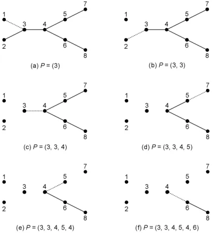
Figure 4 illustrates the encoding process step by step. In Figure 4(a), vertex 1 is the leaf with the lowest label, thus we add its unique neighbor vertex 3 to the sequence, resulting in the Pr¨ufer sequence under construction, denoted by P , equals to (3). Then we remove vertex 1 from the tree. In Figure 4(b), vertex 2 becomes the leaf with the lowest label; we again add its unique neighbor vertex 3 to the sequence. So we have P = (3, 3). After removing vertex 2 from the tree, vertex 3 is the leaf with the lowest label. Since vertex 4 is the unique label of vertex, we get
P = (3, 3, 4). Repeat this operation a few times until only two vertices remain in the tree. In this
example, vertices 6 and 8 are the two vertices left. It follows that the Pr¨ufer sequence for Figure 3 is (3, 3, 4, 5, 4, 6).
It can be verified that different spanning trees of Kndetermine different Pr¨ufer sequences. The Pr¨ufer Decoding algorithm provides the inverse algorithm, which finds the unique labeled tree
T with n vertices for a given Pr¨ufer sequence of n − 2 elements. Let the given Pr¨ufer sequence be
P = (p1, p2, . . . , pn−2). Observe that any vertex v of T occurs deg(v) − 1 times in (p1, p2, . . . , pn−2), where deg(v) is the degree of vertex v. Thus the vertices of degree one, i.e., the leaves, in T are those that do not appear in P . To reconstruct T from (p1, p2, . . . , pn−2), we proceed as follows. Let
V be the vertex label set {1, 2, . . . , n}. In the ith iteration of the for loop, P = (p
i, pi+1, . . . , pn−2). Let v be the smallest element of the set V that does not occur in P . We connect vertex v to vertex
8 1 2 3 4 5 6 7 8 1 2 3 4 5 6 7 8 1 2 3 4 5 6 7 8 1 2 3 4 5 6 7 8 1 2 3 4 5 6 7 (a) P = (3) (b) P = (3, 3) (c) P = (3, 3, 4) (d) P = (3, 3, 4, 5) (e) P = (3, 3, 4, 5, 4) 8 1 2 3 4 5 6 7 (f) P = (3, 3, 4, 5, 4, 6)
Figure 4: Generating a Pr¨ufer sequence from a spanning tree.
pi. Then we remove v from V , and pi from P . Repeat this process for n − 2 times until only two numbers are left in V . Finally, we connect the vertices corresponding to the remaining two numbers in V . It can be shown that different Pr¨ufer sequences deliver different spanning trees of Kn.
Algorithm: Pr¨ufer Decoding
Input: A Pr¨ufer sequence P = (p1, p2, . . . , pn−2).
Output: A labeled tree with vertices labeled by 1, 2, 3, . . . , n.
P ← the input Pr¨ufer sequence
n ← |P | + 2 V ← {1, 2, . . . , n}
Start with n isolated vertices labeled 1, 2, . . . , n. for i = 1 to n − 2 do
v ← the smallest element of the set V that does not occur in P
Connect vertex v to vertex pi Remove v from the set V
Remove the element pi from the sequence P /* Now P = (pi+1, pi+2, . . . , pn−2) */
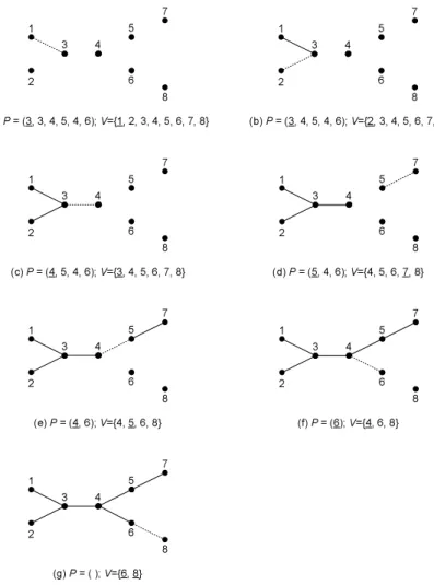
To see how the Pr¨ufer Decoding algorithm works, let us build the spanning tree corre-sponding to the Pr¨ufer sequence (3, 3, 4, 5, 4, 6). Figure 5 illustrates the decoding process step by step. Initially, P = (3, 3, 4, 5, 4, 6) and V = {1, 2, 3, 4, 5, 6, 7}. Vertex 1 is the smallest element of the set V that does not occur in P . Thus we connect vertex 1 to the first element of P , i.e., vertex 3 (see Figure 5(a)). Then we remove 3 from P , and 1 from V . Now P = (3, 4, 5, 4, 6) and
V = {2, 3, 4, 5, 6, 7, 8}. We connect vertex 2 to vertex 3. Repeat this operation again and again
until only two numbers are left in V (see Figure 5(g)).
8 1 2 3 4 5 6 7 (a) P = (3, 3, 4, 5, 4, 6); V={1, 2, 3, 4, 5, 6, 7, 8} 8 1 2 3 4 5 6 7 (b) P = (3, 4, 5, 4, 6); V={2, 3, 4, 5, 6, 7, 8} 8 1 2 3 4 5 6 7 (c) P = (4, 5, 4, 6); V={3, 4, 5, 6, 7, 8} 8 1 2 3 4 5 6 7 (d) P = (5, 4, 6); V={4, 5, 6, 7, 8} 8 1 2 3 4 5 6 7 (e) P = (4, 6); V={4, 5, 6, 8} 8 1 2 3 4 5 6 7 (f) P = (6); V={4, 6, 8} 8 1 2 3 4 5 6 7 (g) P = ( ); V={6, 8}
Figure 5: Recovering a spanning tree from a Pr¨ufer sequence.
We have established a one-to-one correspondence (bijection) between the set of spanning trees of Kn, and the set of Pr¨ufer sequences of length n − 2. We obtain the result in Theorem 2. Theorem 2: The number of spanning trees in Kn is nn−2.
It should be noted that nn−2is the number of distinct spanning trees of K
n, but not the number of nonisomorphic spanning trees of Kn. For example, there are 66−2= 1296 distinct spanning trees of K6, yet there are only six nonisomorphic spanning trees of K6.
In the following, we give a recursive formula for the number of spanning trees in a general graph. Let G − e denote the graph obtained by removing edge e from G. Let G\e denote the resulting graph after contracting e in G. In other words, G\e is the graph obtained by deleting e,
and merging its ends. Let τ (G) denote the number of spanning trees of G. The following recursive formula computes the number of spanning trees in a graph.
Theorem 3: τ (G) = τ (G − e) + τ (G\e)
Proof: The number of spanning trees of G that do not contain e is τ (G − e) since each of them is also a spanning tree of G − e, and vice versa. On the other hand, the number of spanning trees of
G that contain e is τ (G\e) because each of them corresponds to a spanning tree of G\e. Therefore, τ (G) = τ (G − e) + τ (G\e).
References
[1] A. Cayley. A theorem on trees. Quart. J. Math., 23:376–378, 1889.
[2] H. Pr¨ufer. Never beweis eines satzes ¨uber permutationen. Arch. Math. Phys. Sci., 27:742–744, 1918.