A Study on the Min-Max Power-Aware Manycast Routing Problem in Static Ad Hoc Networks
11
0
0
全文
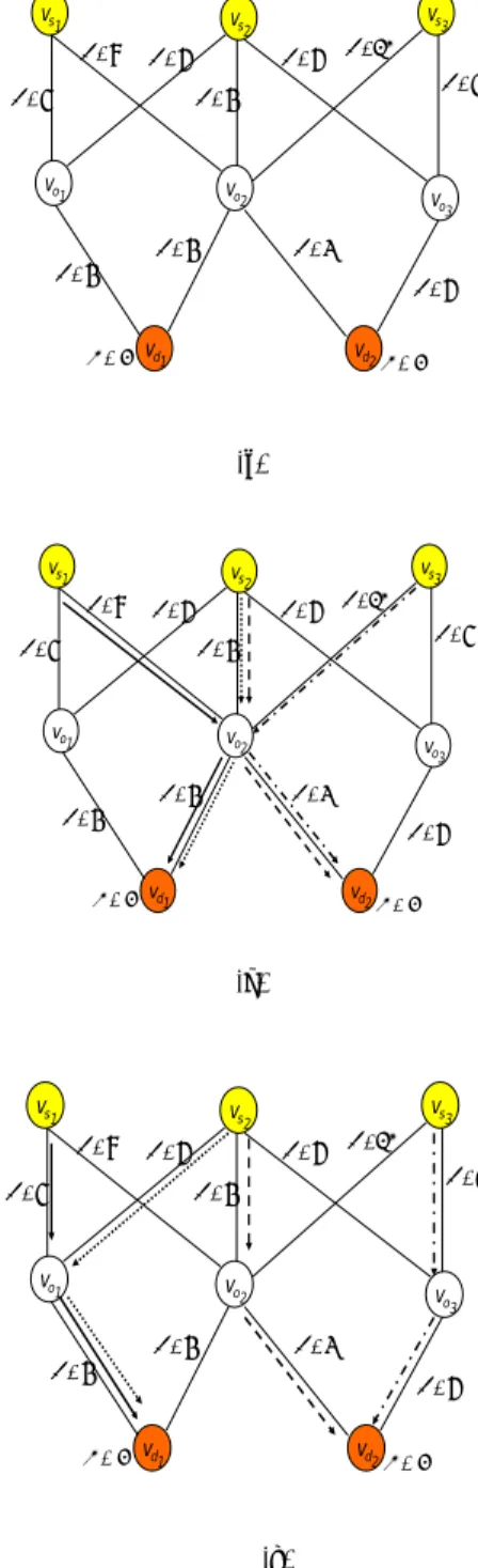
(2) lifetime of network may be shortened significantly. To illustrate the importance of power balance, let us consider the example shown in Figure 2. In Figure 2(a), let nodes vs1 , vs2 , and vs3 be the. imply a longer network lifetime, exemplified by path v1 → v2 → v3 → v4 . On the other hand, we discover that when the power consumptions of nodes even out, the associated network’s lifetime will be longer, as path v1 → v5 → v6 → v4 shows. In this paper, we will take the approach of leveling each node’s power consumptions as a starting point. In ad hoc networks, common communication models among hosts include unicast (one-to-one) transmission, anycast (one-to-any) transmission [1][6][10][11], multicast (one-to-many) transmission, and broadcast (one-to-all) transmission. Besides, manycast transmission has been comprehensively investigated and become an important communication model recently [3]. In fact, manycast transmission is a group communication model in which a number of servers (or called source nodes) provide the same type of services and resources. When a client (or called a destination node) wants to get services or resources, the manycast routing algorithm will arrange a set of suitable servers to it, i.e., one client will communication with multiple ( k ≥ 1 ) servers at the same time, where k is specified by each client. Notice that when k = 1 for each client, manycast transmission becomes anycast transmission. That is, anycast transmission is a special case of manycast transmission. At present, there exist a lot of network applications which adopt manycast transmission. For example, a distributed certificate authority for wired networks has been established by COCA (Cornell On-Line Certification Authority) [17]. Furthermore, such a system has been extended to wireless ad hoc networks by MOCA (Mobile Certificate Authorities) [16]. On three distributed examination key systems, authority is distributed across several servers using threshold cryptography. Therefore a client must contact several servers simultaneously for certification [3]. When designing manycast routing algorithms for ad hoc networks, we must take the main characteristic of ad hoc networks into consideration: the battery power of each host is very limited. If the routing requirements are arranged by those manycast routing algorithms only armed with shortest-path routing paths, individual power consumption may vary although the total transmission power consumption is smaller. As a result, the network may suffer very short lifetime. Instead, if we attempt to evenly distribute packet-relaying loads among nodes to prevent the overuse or abuse of battery power [8][9][12][14], we believe that the network’s lifetime will be extended significantly. For example, in the above distributed certificate authority system, when the requirements of most clients are satisfied by the same set of servers, the battery power of some nodes (including source nodes and intermediate nodes) may be consumed abnormally quickly, which implies the. source nodes and nodes vd1. and vd 2. be the. destination nodes, respectively. The number next to each link represents the power to be consumed when one connection is delivered through the link. Now, consider that each destination node will require two connections. If the routing paths are allocated as shown in Figure 2(b), obviously, the power of node vo2 will be overused and the network’s lifetime may become very short. On the other hand, if the routing paths are allocated carefully, as Figure 2(c) shows, the power consumption of each node will be more balanced. In this case, we are convinced of a longer network’s lifetime. In this paper we will thus define our goal of study: designing an efficient manycast routing algorithm to arrange manycast transmission requirements such that the power consumption of each node is as balanced as possible. We will call it the min-max power-aware manycast routing (MMPAMR) problem. To be more specific, given a set of destination nodes each of which requires a different amount of connections, find a set of routing paths between the given source nodes and the given destination nodes such that the power consumption of each node in the network is as even as possible. Undoubtedly, the resulted lifetime of network is extended. While it is easy to find a set of routing paths with the minimal total transmission power consumption to satisfy the connection requirement of each destination hosts, in this paper we will prove that the MMPAMR problem is NP-complete. To solve the difficult MMPAMR problem, based on Dijkstra’s algorithm, an efficient heuristic algorithm with low time complexity is developed. Computer simulations verify that the lifetimes of networks generated by our power-balanced manycast routing algorithm are longer than those generated by our another shortest-path-based manycast routing algorithm. The rest of the paper is organized as follows. In Section 2, a formal definition of our MMPAMR problem is given. In Section 3, our MMPAMR problem is proved to be NP-complete. In Section 4, efficient heuristic algorithms for the MMPAMR problem are proposed. In Section 5, the performances of our heuristic algorithms are evaluated through computer simulations. Lastly, Section 6 concludes the whole research.. 2. The Definition of our MMPAMR Problem In this section, we will introduce our some 2.
(3) assumptions, notations, and definitions. A formal definition of our problem in terms of these notations and definitions will also been stated. In the following, the term “node” is synonymous with the term “host” and the term “link” is synonymous with the term “communication channel”.. connections required by all the destination nodes. Based on these notations and definitions, now we can formally describe our min-max power-aware manycast routing (MMPAMR) problem as follows: given a weighted graph G=(V,E), a set of source hosts S = {vs1 , vs2 ,..., vsm } and a set of destination hosts. 2.1 Assumptions. D = {vd1 , vd2 ,..., vdn } , a connection requirement. The following states some important assumptions used in our research. (1) We assume that the ad hoc network’s topology would not change, i.e. no host gets move. The assumption has been adopted in [2][9][15]. (2) We only consider the transmission power and ignore the reception power. The assumption has been adopted in [5]. (3) We assume that the required transmission power to establish a communication channel between any two hosts x and y is the same. In other words, c(< v x , v y >) = c(< v y , v x >) , where c(< v x , v y >). function γ : D → I+ , a transmission power consumption function β : E → R , find a set of routing paths such that (1) the connection requirement function of each destination node is satisfied, (2) each source provides at most one connection to each destination, and (3) the maximum of node’s transmission power consumption in G is +. {. }. minimized , i.e., max α ( vi ) vi ∈G. is minimized.. respectively. The assumption has been adopted in [5]. (4) We assume that when one connection passes through a link, the transmission power consumption associated with the link can be an arbitrary value, i.e., can be independent of the Euclidean length of link. The assumption has adopted in [2][5].. As an example, let us consider Figure 2(a) again, where an ad hoc network is shown with three source nodes and two destination nodes. The number next to each node represents the number of connections required by the node. The number next to each link represents the power to be consumed when one connection is delivered through the link. Figure 3 shows a set of routing paths with the best power balance. In this case, the maximum of node’s transmission power consumption in the network max α ( vi ) is equal to α (vs2 ) = 4 + 4 = 8,. 2.2 Problem Formulation. which is the best solution.. and c(< v y , v x >) denote the minimal transmission power required by hosts x and y to establish communication channels < v x , v y > and < v y , v x > ,. vi ∈G. We represent an ad hoc network by a weighted graph G = (V, E), where V denotes the set of hosts (including source hosts, destination hosts, and intermediating hosts) and E denotes the set of communication channels connecting the hosts. Let D = {vd1 , vd2 ,..., v dn } be a set of destination hosts.. In this section, we will show that our MMPAMR problem is NP-complete. To prove our MMPAMR problem to be NP-complete, first let us restate it in its decision version as follows: given a weighted graph G=(V,E), a set of source hosts S = {vs1 , vs2 ,..., vsm } , a. of connections required by destination vdi . For E,. set of destination hosts D = {vd1 , vd 2 ,..., vdn } , a. we define a transmission power consumption function. connection requirement function γ : D → I + , a. +. : E → R that assigns a nonnegative weight to each link in the network. The value β (vi , v j ) associated with link (vi , v j ) ∈ E represents the transmission power that node. }. 3. The Complexity of our MMPAMR Problem. For D, we define a connection requirement function γ : D → I + . The value γ (vdi ) represents the number. β. {. transmission power consumption function. β. E→. :. +. R , a power-constrained constant c p , find a set of routing paths such that (1) the connection requirement function of each destination node is satisfied, (2) each source provides at most one connection to each destination, and (3) the maximum of node’s transmission power consumption in G is. vi will. consume when one connection is delivered through that link. For E, we define a connection flow function f : E → I + . The valu e f (vi , v j ) denotes the. {. }. number of connections passing through link (vi , v j ) .. less than or equal to c p , i.e., max α ( vi ). For V, we define a node power consumption function α :V → R + . Thus, α (vi ) = ∑ f (vi , v j ) × β (vi , v j ). c p .For simplicity, in what follows, we will not. vi ∈G. distinguish the decision version and the optimal version of the MMPAMR problem when no ambiguity arises. Next, let us introduce the 3-Dimensional. ( vi , v j )∈E. represents the total transmission power that node. ≤. vi. will consume during the deliveries of all the 3.
(4) M′ a g r e e i n a n y c o o r d i n a t e . I f wi′, x′j , yk′ ∈ M ′ , then we let vwi′ , vx′j , v yk′. Matching (3DM) problem [7]. Instance: A set M ⊆ W × X × Y , where W, X, and Y are disjoint sets having the same number q of elements. Question: Does M contain a matching, that is, a. (. one of these q paths. Therefore, for each link (vi , v j ) ∈ E , f (vi , v j ) ≤ 1 . Similarly, any node vi belongs to at most one of these q paths. So, for any vi ∈V , ∑ f ( vi , v j ) ≤ 1 . Thus, for any vi ∈V ,. W = X = Y = q , and M ⊆ W × X × Y be. ( vi , v j ) ∈ E. we have α(vi ) =. an arbitrary instance of 3DM. Let the elements of these sets be denoted by , X = x1, x2, , xq W= w1, w2, , wq. ,Y ={ y1, y2, , yq} and. M = {m1 , m2 ,. vi ∈G. ( vi , v j )∈E. 1× f (vi , v j ) ≤ 1 .. α (vi ) ≤ 1. for. vi . Furthermore, each link has a transmission power consumption of 1, each node vi each node. belongs to at most one path Pl. ∪ { v y1 , v y2 ,… , v yq }. If. α ( vi ) > c p = 1 ). Thus paths. (. wi , x j , yk ) ∈ M, then there exist one edge. Pt = ( vwt , v xt , v yt ) , then let i. edge < v x j , v yk > between nodes v x j and v yk .. j. k. (otherwise,. P1 , P2 ,. pairwise node-disjoint. If Pt ∈ P1 , P2 ,. < vwi , v x j > between nodes v wi and v x j , and one. , Pq. are. ). , Pq , where. (w , x , y )∈ M ′ ti. tj. tk. .. Clearly M ′ = q, M ′ ⊆ M, and no two elements of M ′ agree in any coordinate. Thus, M ′ is a matching. This completes our proof of NP-completeness. ▓ From the proof of Theorem 1, we can obtain the following results easily. Corollary 1. The MMPAMR problem is strongly NP-complete. That is, the problem remains NP-complete even if the transmission power consumption of each line is constrained to be below a given constant. Corollary 2. The MMPAMR problem is still NP-complete even when the transmission power consumptions of all the lines are the same. When a problem is proved to be NP-complete, the follow-up quest will be to search for various heuristic algorithms for the problem and evaluate them by computer simulations. In the next section, we will design efficient heuristic algorithms for the. Thus, the edge set E = { < vwi , v x j > : if. wi , x j , yk ) ∈ M }∪{ < v x j , v yk > : if yk ) ∈ M }. The number of connections. required by each destination node v yk is assumed to be. j. B e c a u s e max{α (vi )} ≤ 1 = c p ,. (an. (1 ≤ i ≤ q). Thus, V = { vw1 , vw2 ,… , vwq } ∪. ( wi , x j ,. i. be one of the possible solutions in G .. intermediate nodes v xi , a destination node v yi ). (. j. routing paths form a set of feasible routing paths for the corresponding MMPAMR problem in G . Next, suppose we have a solution for the MMPAMR problem in the weighted graph G. Let P1 , P2 , , Pq. MMPAMR problem as follows: For each element wi ( xi , yi ) of W, the corresponding weighted. (. i. vi ∈G. where k = M . We construct an instance of the. { vx1 , vx2 ,… , vxq }. ∑ β(v ,v )×f (v ,v ) = ∑. (vi ,vj )∈E. As a result, max{α (vi )} ≤ 1 = c p . Thus, these q. }. , mk } ,. graph G = (V, E) has a source node v wi. vwi′. q routing paths each of which is for a different pair of source and destination nodes. Since no two elements of M ′ agree in any coordinate, these routing paths are pairwise node-disjoint. Because they are pairwise node-disjoint, any link ( vi , v j ) belongs to at most. This problem was shown to be NP-complete by Karp [7]. Now, we will use it to prove the following theorem. Theorem 1. The MMPAMR problem is NP-complete. Proof. First, the MMPAMR problem can be easily seen to be in the class NP. We next transform the 3DM problem to the MMPAMR problem in polynomial time. Let the sets W, X, Y, with. {. ). and destination node v yk′ . Since M ′ = q , there are. M ′ ⊆ M such that M ′ = q and no two elements of M ′ agree in any coordinate?. }. (. be a routing path in G between source node. subset. {. ). γ ( v y ) = 1 . Each edge has a transmission power k. consumption of 1 when one connection traverses it. Finally, let c p =1. The constructed G is illustrated in Figure 4. It is easy to see that this transformation can be finished in polynomial time. We next show that there exists a set of feasible routing paths for the MMPAMR problem in G if and only if the set M contains a matching M ′ . First, suppose M contains a matching, that is, a subset. M ′ ⊆ M such that M ′ = q and no two elements of 4.
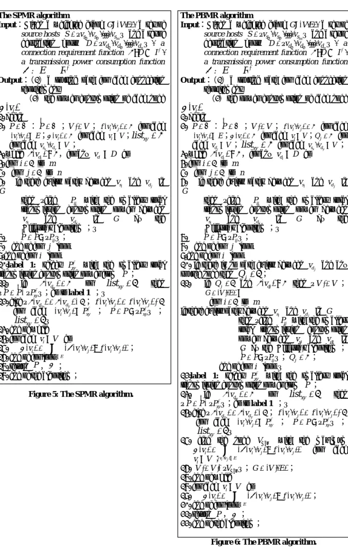
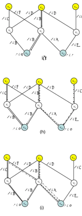
(5) MMPAMR problems.. represents that node vd y will be able not to establish. 4. Efficient Heuristic Algorithms for the MMPAMR Problem. any connection to node vsx in the following rounds). Line 4 to line 9 are used to find the shortest path for each pair of source and destination. Line 11 makes V ' to be recovered from V when there doesn’t exist any path to connect the destination vd j with. In this section, we will propose two heuristic algorithms for the MMPAMR problem. One is simpler and faster while the other is more efficient. The first one is based on a shortest path algorithm, and we call it the shortest path manycast routing algorithm (the SPMR algorithm, for short). The other is a routing algorithm with power-balanced, and we call it the power-balanced manycast routing algorithm (the PBMR algorithm, for short). The spirit of the SPMR algorithm is to use the Dijkstra’s algorithm to satisfy each connection requirement. Figure 5 is the description of the SPMR algorithm. The P in line 2 is to save the set of the. non-zero remaining connection requirements to any source. And then we will search the shortest paths for vd j to all the source nodes. Line 12 to line 14 search the routing path with the minimal power consumption ^. among the routing paths existing in set P to establish the connection, and set list xy =1 where. vsx is the source node and vd y is the destination node.. ^. routing path for all the connection requirements, P is to save the set of the shortest paths in each round, and list xy records the connection status ( list xy =1. Line 15 removes the node with maximal transmission power consumption in the network and produces a new graph G = (V ', E ) . The process will not stop until we obtain the routing paths for all the connection requirements. Line 18 to line 20 compute the transmission power consumption of each node. Line 21 outputs the set of routing paths P and the transmission power consumption of each node.. represents that node vd y will be not able to establish any connection to node vsx in the following rounds). Line 4 to line 9 are to find the shortest path for each pair of source and destination. Line 10 to line 12 search the routing path with the minimal power consumption among the routing paths existing in set. Example We will explain the operation of our PBMR algorithm by using Figure 7. In Figure 7(a), let nodes vs1 , vs2 , and vs3 be the source nodes and nodes vd1. ^. P to establish the connection, and set list xy =1 where vsx is the source node and vd y is the. and vd 2 be the destination nodes, respectively. The. destination node. The process will not stop until we generate the routing paths for all the connection requirements. Line 14 to line 16 compute the transmission power consumption of each node. Line 18 outputs the set of routing paths P and the transmission power consumption of each node. Our second heuristic algorithm, the PBMR algorithm, is to improve the SPMR algorithm. We discover that the power of some nodes will be overused when most routing paths bypass the same set of nodes. This will result in decreasing the lifetime of network. The basic idea of our PBMR algorithm is as follows: after one connection is established, we remove the node with maximal transmission power consumption in the network temporarily to prevent the overuse of this node. Figure 6 is the description of our PBMR algorithm. The P in line 2 is used to save the set of the. number next to each link represents the power to be consumed when one connection bypasses this link. Now, consider that each destination node will require two connections. First of all, we will find the shortest paths for each pair of source and destination, shown as Figure 7(b). In Figure 7(c), we select the routing path with minimal power consumption from the set of routing paths and set it as the first routing path for all the connection requirements. Next, we will remove the node with the maximal transmission power consumption in the network, which is node is v2 . We repeat this process until all the connection requirements are satisfied. In Figure 7(f), there is one connection requirement for vd1 yet and we can not find any routing path for vd1 . At this time, we will use the original graph G to find the shortest paths from all the source nodes to vd1 , and then repeat the. ^. routing path for all the connection requirements, P is used to save the set of the shortest paths in each round, Q j is used to indicate whether there are. process we mention before, shown in Figure 7(g). Figure 7(h) shows the result produced by our PBMR algorithm while Figure 7(i) shows the result produced by our SPMR algorithm. We can see that the node with maximal transmission power consumption obtained by our PBMR algorithm is vs2 , whose. paths connect the node vd j to any source node, V ' is the set of residual nodes after each round, and list xy is to record the connection status ( list xy =1 5.
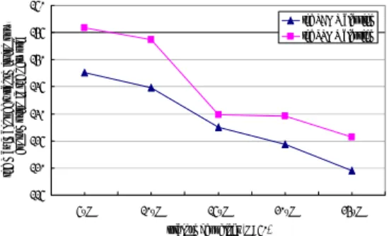
(6) α (vs ) is 8. On the other hand, the node with. set as follows: the network consists of 50 nodes which are located in a 100 × 100 m2 area randomly. The transmission power consumption of each link is assigned to a value between 10 and 40 randomly. The number of source nodes is set to 20 and the number of destination nodes is set to 10. The number of connections required by each destination node is assigned to a value between 1 and 10 randomly. In our second simulation environment, we will observe how the total number of links impacts on the performances of the two heuristic algorithms. From Figure 9(a) (where N denotes the total number of nodes in the network, and in this case N is 50), it can be easily found that the maximal node’s transmission power consumption of the two heuristic algorithms decrease with the raising of the total number of links. This is because the more the total number of links is, there are more chances for the manycast routing algorithms to select the proper routing paths each destination node. The maximal node’s transmission power consumption obtained by PBRM algorithm is also lower than the values obtained by the SPMR algorithm. Figure 9(b) shows our PBMR algorithm has longer lifetime than the SPMR algorithm. The environments in our third simulation are set as follows: the network consists of variant numbers of nodes which are located in a 100 × 100 m2 area randomly. The number of links is set to N × ( N − 1) / 4 (where N denotes the total number of nodes). The transmission power consumption of each link is assigned to a value between 10 and 40 randomly. The number of source nodes is set to 20 and the number of destination nodes is set to 10. The number of connections required by each destination node is assigned to a value between 1 and 10 randomly. In our third simulation environment, we will observe how the size of network impacts on the performances of our PBRM algorithm and the SPMR algorithm. Figure 10 gives the simulation results when the total number of nodes varies from 60 to 100. Figure 10(a) and Figure 10(b) tell us that the size of network doesn’t affect the performances of these two algorithms too much. The environments in our fourth simulation are set as follows: the network consists of variant numbers of nodes which are located in a 100 × 100 m2 area randomly. The total number of nodes varies from 20 to 100. The number of links is set to N × ( N − 1) / 4 (where N denotes the total number of nodes in network). The transmission power consumption of a links is assigned to a value between 10 and 40 randomly. The number of source nodes is set to 1 / 2 × N , and the number of destination nodes is set to 1 / 4 × N . The number of connections required by each destination node is assigned to a value between 1 and 10 randomly. In our forth simulation environment, we will observe how the. 1. maximal transmission power consumption obtained by the SPMR algorithm is vs1 , whose α (vs1 ) is 13. Therefore, we can see that our PBMR algorithm is more efficient than the SPMR algorithm. We will further justify the fact by the computer simulation in Section 5.. 5. Computer Simulations In this section, by means of computer simulations, we will examine the efficiency of the SPMR algorithm and the PBMR algorithm. We will observe the maximal node’s power consumption in the network and the network’s lifetime. The lifetime residual power of network is measured in terms of max{α (vi )} vi ∈V. (where we set the residual power of each node to be 10000), i.e., the connections have been successfully established from their sources to their destinations during the time period from the beginning of network’s operation to the time when the first node exhausts its residual power.. 5.1 Simulation Results In this subsection, we will present and discuss the simulation results of the SPMR algorithm and the PBMR algorithm in four different simulation environments. The environments in our first simulation are set as follows: the network consists of 100 nodes which are located in a 100 × 100 m2 area randomly. The number of links is set to N × ( N − 1) / 4 , where N is 100. The transmission power consumption of each link is assigned to a value between 10 and 40 randomly. The number of destination nodes is set to 10. The number of connections required by each destination node is assigned to a value between 1 and 10 randomly. In our first simulation environment, we will observe how the number of source nodes impacts on the performances of our PBMR algorithm and the SPMR algorithm. Figure 8 shows the simulation results, where we vary the number of source nodes from 10 to 50. From Figure 8(a), it can be found that the maximal node’s power transmission consumption in the network produced by our PBMR is much lower than those produced by the SPMR algorithms. We can also observe that the maximal node’s transmission power consumption decreases with the raising of the number of source nodes. This is because the more source nodes exist, there are more chances for manycast routing algorithms to select the proper source nodes to establish connections to each destination node. From Figure 8(b), we can see that our PBMR algorithm has longer lifetime than the SPMR algorithm before the first node shuts down (i.e. the first node exhausts its residual power). The environments in our second simulation are 6.
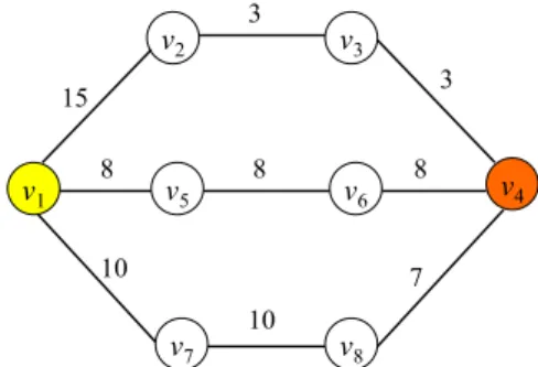
(7) [7] M. R. Garey and D. S. Johnson, Computers and Intractability: A Guide to the Theory of NP-Completeness, San Francisco: W. H. Freeman & Company, Publishers, 1979. [8] A. Michail and A. Ephremides, "Energy Efficient Routing for Connection-Oriented Traffic in Ad Hoc Wireless Networks," The 11th IEEE International Symposium on Personal, Indoor, and Mobile Radio Communications (PIMRC 2000), vol. 2, pp.762-766, September 2000. [9] A. Misra and S. Banerjee, "MRPC: Maximizing Network Lifetime for Reliable Routing in Wireless Environments," WCNC, pp. 800-806, March 2002. [10] V. D. Park and J. P. Macker, "Anycast Routing for Mobile Networking," Proceedings of the Military Communications International Symposium (MILCOM’99), November 1999. [11] H. Sarhan and C. Yu, "IP Anycast in Ad Hoc Networks," MCRL (Mobile Computing Research Lab.), ECE Dept., CSU, September 2002. [12] S. Singh, M. Woo, and C. S. Raghavendra, "Power-Aware Routing in Mobile Ad Hoc Networks," Proceedings of the MobiCom’98, October 1998. [13] C. Siva Ram Murthy and B.S. Manoj, Ad Hoc Wireless Networks: Architectures and Protocols, Prentice Hall, 2004. [14] C. K. Toh, "Maximum Battery Life Routing to Support Ubiquitous Mobile Computing in Wireless Ad Hoc Networks," IEEE Communications Magazine, vol. 39, pp.138-147, June 2001. [15] J. E. Wieselthier, G. D. Nguyen, and A. Ephremides, "On the Construction of Energy-Efficient Broadcast and Multicast Trees in Wireless Networks," Proceedings of the 19th IEEE INFOCOM, pp. 585-594, 2000. [16] S. Yi and R. Kravets, "MOCA: Mobile Certificate Authority for Wireless Ad Hoc Networks," In 2nd Annual PKI Research Workshop (PKI03), April 2003. [17] L. Zhou, F. B. Schneider, and R. van Renesse, "COCA: Asecure Distributed On-Line Certification Authority," ACM Transactions on Computer Systems, vol. 20, no. 4, pp. 329–368, November 2002.. structure of network impacts on the performances of the two heuristic algorithms. Figure 11(a) and Figure 11(b) show that the maximal node’s transmission power consumption of the two heuristic algorithms decreases with the raising of the total number of nodes. Because the number of connections required by each destination node is fixed, the power of each node in the network with small structure will may be overused. That is, the larger the structure is, the lower the maximal node’s transmission power consumption is.. 6. Conclusions In this paper, we have shown the MMPAMR problem to be NP-complete. Based on the Dijkstra’s algorithm, two heuristic algorithms with low time complexities have been developed. The SPMR algorithm is simpler and faster while the PBMR algorithm is more efficient. Computer simulations verify that of the PBMR algorithm is more efficient than the SPMR algorithm.. Acknowledgements This work was supported by the National Science Council of the Republic of China under Grant # NSC 93-2213-E-224-023. References [1] P. Basu, W. Ke, and T. D. C. Little, "Dynamic Task-Based Anycasting in Mobile Ad Hoc Networks," Mobile Networks and Applications, vol. 8 no. 5, pp. 593 - 612 , 2003. [2] M. Cagalj, J. P. Hubaux, and C. Enz, "Minimum-Energy Broadcast in All-Wireless Networks: NP-Completeness and Distribution Issues," Proceedings of the Eighth ACM International Conference on Mobile Computing and Networking (Mobicom 2002), September 2002. [3] C. Carter, S. Yi, P.t Ratanchandani, and R. Kravets, "Manycast: Exploring the Space Between Anycast and Multicast in Ad Hoc Networks," Proceedings of the 9th annual international conference on Mobile computing and networking, pp. 273 - 285 , September 2003. [4] J. H. Chang and L. Tassiulas, "Energy Conserving Routing in Wireless Ad-Hoc Networks," INFOCOM 2000, Nineteenth Annual Joint Conference of the IEEE Computers and Communications Societies, vol. 1, pp. 22-31, 2000. [5] W. T. Chen and N. F. Huang, "The Strongly Connecting Problem on Multihop Packet Radio Networks, " IEEE Transactions on Communications, vol. 37, no. 3, pp. 293-295, March 1989. [6] R. R. Choudhury and N. H. Vaidya, "MAC-Layer Anycasting in Ad Hoc Networks," ACM SIGCOMM Computer Communication Review, vol. 34, no. 1, pp. 75 – 80, January 2004.. 3. v2. v3 3. 15. v1. 8. v5. 8. v6. 10. 8. v4. 7 10. v7. v8. Figure 1: A smaller total transmission power does not always imply a longer network’s lifetime.. 7.
(8) α(vs ) = 4+ 4 = 8 2. vs. β =8. 2. 3. β = 6 β =10. β =6. β =5. vo. 1. β =5. β =4. vo. 2. β =4. vd. vo. vo. 3. β =4. β =3 β =6. γ = 2 v d1. (a). 3. β =5. vo2. 1. β =4. γ =2. 2. vs. β = 6 β =10. β =4. 3. β =6. 2. β =6. β =5. β =3. γ = 2 v d1. vs. 1. β =8. β =4. vo. vs. vs. vs. 1. v d2. γ =2. Figure 3: An illustration of our MMPAMR problem.. vs. β =8. vs. vs2. 1. β =5. 3. β = 6 β =10. β =6. β =5. β =4. vo1. vo2. β =4. vw1. vo3. β =4. β =1. γ = 2 vd1. vd. 2. β =1. γ =2. β =8. β =6. β =5. β = 6 β =10. vo2. β =4. vo. β =4. β =1. β =1. β =5. β =4. vo1. vwq-1. . . .. v wq. γ =1. vy2. γ =1. β =1 β =1. . . .. vxq-1. β =1 β =1. β =1. vx3. vy1. β =1. β =1. β =1. . . .. vs3. β =1 vx2. β =1. vw3. (b). vs2. β =1. vw2. β =1. vx1. β =1. β =3 β =6. vs1. β =1. β =1. γ =1. vyq-1. γ =1. β =1. β =1 vxq. vy3. β =1. v yq. γ =1. c p =1. 3. β =3 β =6. γ = 2 vd1. vd. 2. Figure 4: An illustration of Theorem 1.. γ =2. (c). Figure 2: The importance of power balance.. 8.
(9) The SPMR algorithm Input:Given a weighted graph G=(V,E), a set of source hosts S = {vs1 , vs2 ,..., vsm } and a set of destination hosts D = {vd1 , vd 2 ,..., vdn } , a connection requirement function γ : D → I + , a transmission power consumption function β : E → R+ Output:( 1 ) a routing path for each connection requirement (2)the power consumption of each node. The PBMR algorithm Input:Given a weighted graph G=(V,E), a set of source hosts S = {vs1 , vs2 ,..., vsm } and a set of destination hosts D = {vd1 , vd 2 ,..., vdn } , a connection requirement function γ : D → I + , a transmission power consumption function β : E → R+ Output:( 1 ) a routing path for each connection requirement (2)the power consumption of each node. 1. begin ^ 2. P = Φ : P = Φ ; V ' = V ; f (vi , v j ) = 0 for each (vi , v j ) ∈ E ;α (vi ) = 0 for each vi ∈ V ;list xy = 0 for each vs , vd ∈ V ; 3. while γ (vdi ) ≠ 0 ,for any vd ∈ D do 4. for i = 1 to m 5. for j = 1 to n 6. if there exists paths between vsi and vd j in G Pij with the smallest total then {find transmission consumption power between vsi and in by the vd j G Dijkstra's algorithm ;} ^ ^ 7. P = P∪ {Pij } ; 8. end of for j loop 9.end of for i loop 10.label 1: select Pxy' with the smallest total ^ transmission consumption power from P ; 11.^ ^ if or then γ (vd y ) = 0 list xy = 1 { P = P − {Pxy' } ;go to label 1 ;} 12. else { γ (vd y ) = γ (vd y ) − 1 ; f (vi , v j ) = f (vi , v j ) + 1 for each (vi , v j ) ∈ Pxy' ; P = P ∪ {Pxy' } ; list xy = 1 } 13. end of while 14. for each vi ∈ V do 15. α (vi ) = ∑ ( β (vi , v j ) × f (vi , v j )) ; ( vi , v j )∈E 16. end of for loop P 17. return ,α ; 18. end of the algorithm;. 1. begin ^ 2. P = Φ : P = Φ ; V ' = V ; f (vi , v j ) = 0 for each (vi , v j ) ∈ E ;α (vi ) = 0 for each vi ∈ V ;Q j = 0 for each vd ∈ V ; list xy = 0 for each vs , vd ∈ V ; 3. while γ (vdi ) ≠ 0 ,for any vdi ∈ D do 4. for i = 1 to m 5. for j = 1 to n 6. if there exists paths between vsi and vd j in G Pij with the smallest total then {find transmission consumption power between vsi and in by the vd j G Dijkstra's algorithm ;} ^ ^ 7. P = P ∪ {Pij } ; 8. end of for j loop 9.end of for i loop 10. if there is no path exists between vd j and any source node then Q j = 1 ; 11. if Q j = 1 and γ (vdj ) ≠ 0 then { V ' = V ; G = (V ', E ) ; for i = 1 to m if there exists paths between vsi and vd j in G then {find Pij with the smallest total transmission consumption power between vsi and vdj in by the Dijkstra's algorithm ; G ^ ^ P = P∪ {Pij } ; Q j = 0 ; end of for i loop } 12.label 1: select Pxy' with the smallest total ^ transmission consumption power from P ; 13.^ ^ if or then γ (vd y ) = 0 list xy = 1 { P = P − {Pxy' } ;go to label 1 ;} 14. else { γ (vd y ) = γ (vd y ) − 1 ; f (vi , v j ) = f (vi , v j ) + 1 for each (vi , v j ) ∈ Pxy' ; P = P ∪ {Pxy' } ; list xy = 1 } 15. find the node Vmax with the maximum α (vi ) = ∑ ( β (vi , v j ) × f (vi , v j )) for each ( vi , v j )∈E vi ∈ V ; 16. V ' = V '− {Vmax } ; G = (V ', E ) ; 17. end of while 18. for each vi ∈ V do 19. α (vi ) = ∑ ( β (vi , v j ) × f (vi , v j )) ; ( vi , v j )∈E 20. end of for loop 21. return P , α ; 22. end of the algorithm;. α (vi ). x. α (vi ). y. j. Figure 5: The SPMR algorithm.. x. Figure 6: The PBMR algorithm.. 9. y.
(10) Vs1. β =6. β =5. β =4. V1. V2. β =4. V1. β =3. Vd1. Vd2. (a). Vs1. β =6. β =4. β =5. V1. β =5. V2. β =4 γ = 2. (b). Vs1. β =6. β =4 γ = 2. β =5. β =4. V2. β =7 Vd2. (h). γ = 2. β =6. Vs3. β =5. β =6. β =5. β =4. V2. V3. V3. β =4. β =4. V3. β =3. Vd1. V1. V1. β =5. Vs2. β =8. β =5. β =4. Vs3. β =6. Vs1. Vs3. β =6. γ =0. V2. γ = 2. Vs2. β =8. β =6. V1. β =7 Vd2. (g). β =4. β =3. Vd1. Vd2. β =5. V3. β =4. β =7 Vd1. Vs2. β =8. β =4. β =3. Vs1. Vs3. V3. β =4. γ =1. β =6. β =5. V2. γ = 2. Vs2. β =8. β =6 β =4. β =7. γ = 2. β =6. β =5. V3. β =4. Vs3. Vs2. β =8. β =6. β =5. Vs1. Vs3. Vs2. β =8. β =3. β =4. β =4. β =3 β =7. β =7. γ = 2. Vd1. Vd2. (c). γ = 2. γ = 2. Vd1. Vd2. (i). γ = 2. Figure 7: An example to illustrate the operation of x. β =6x. β =5. β =6. β =4. β =5. x. x V1. 180. V2. V3. β =4. β =4. β =3 β =7. γ = 2. Vd1. Vd2. (d). x. γ =1. x. Vs1. Vs3. Vs2. xβ = 8. x. β =6. β =5. β =6. β =4. x. x. V1. β =5. x. V2. β =4. β =4. 160 150 140 130 120 110 100 90 80 70 60 10. V3. 20. 30. 40. 50. the number of source nodes β =7. γ =1. Vd1. Vd2. (e). x. transmission power consumption in the network Vs3. Vs2. xβ = 8. β =6. x. β =5. x. β =6 β =4. x. V1. (a)The effect of the number of source nodes on the maximal node’s. γ =1. x. Vs1. x. the PBMR algorithm the SPMR algorithm. 170. β =3. β =4 γ =1. 140. V3. x. x. β =3. β =7 Vd1. Vd2. (f). the PBMR algorithm the SPMR algorithm. 130. V2. β =4. 150. β =5. x. the lifetime of netw ork. x. the PBMR algorithm.. Vs3. Vs2. β =8. the m aximal node's transmission pow e consumption in the netw ork. Vs1. γ = 0. 120 110 100 90 80 70 60 50 10. 20. 30. 40. 50. the number of source nodes. (b)The effect of the number of source nodes on the lifetime of network. Figure 8: The influence of the number of source nodes.. 10.
(11) 175. the PBMR algorithm the SPMR algorithm. 145. th e m ax im al n o d e's tran sm issio n p o w e con su m p tion in th e n etw o rk. the maximal node's transmission powe consumption in the netw ork. 150. 140 135 130 125 120 115 5×N. 10×N. 15×N. 20×N. 24×N. the PBMR algorithm. 170. the SPMR algorithm. 165 160 155 150 145 140 135 130. total number of links (N=50). 20. 40. (a)The effect of the total number of links on the maximal node’s transmission power consumption in the network. 76. 80. 74. 78. th e lifetim e o f n etw o rk. the lifetime of netw ork. 82. 76 74 72 70 10×N. 100. transmission power consumption in the network. the PBMR algorithm the SPMR algorithm. 5×N. 80. (a)The effect of the structure of network on the maximal node’s. 86 84. 60 total number of nodes. 15×N. 20×N. 24×N. the PBMR algorithm the SPMR algorithm. 72 70 68 66 64. total number of links (N=50). 62 60 20. (b)The effect of the total number of links on the lifetime of. 40. 60. 80. 100. total number of nodes. network Figure 9: The influence of the total number of links.. (b)The effect of the structure of network on the lifetime of network the maximal node's transmission powe consumption in the network. 135. Figure 11: The influence of the structure of network.. 133. the PBMR algorithm the SPMR algorithm. 131 129 127 125 123 121 119 117 115 60. 70. 80. 90. 100. total number of nodes. (a)The effect of the size of network on the maximal node’s transmission power consumption in the network 88. the lifetime of netw ork. 86. the PBMR algorithm the SPMR algorithm. 84 82 80 78 76 74 60. 70. 80. 90. 100. total number of nodes. (b)The effect of the size of network on the lifetime of network Figure 10: The influence of the size of network.. 11.
(12)
數據
+2
相關文件
6 《中論·觀因緣品》,《佛藏要籍選刊》第 9 冊,上海古籍出版社 1994 年版,第 1
The first row shows the eyespot with white inner ring, black middle ring, and yellow outer ring in Bicyclus anynana.. The second row provides the eyespot with black inner ring
The underlying idea was to use the power of sampling, in a fashion similar to the way it is used in empirical samples from large universes of data, in order to approximate the
Write the following problem on the board: “What is the area of the largest rectangle that can be inscribed in a circle of radius 4?” Have one half of the class try to solve this
Teachers may consider the school’s aims and conditions or even the language environment to select the most appropriate approach according to students’ need and ability; or develop
Robinson Crusoe is an Englishman from the 1) t_______ of York in the seventeenth century, the youngest son of a merchant of German origin. This trip is financially successful,
fostering independent application of reading strategies Strategy 7: Provide opportunities for students to track, reflect on, and share their learning progress (destination). •
Now, nearly all of the current flows through wire S since it has a much lower resistance than the light bulb. The light bulb does not glow because the current flowing through it
