An Efficient Algorithm for Determining the Dispersion Characteristics of Single-Mode Optical Fibers

JOURNAL OF LIGHTWAVE TECHNOLOGY, VOL. 10, NO. 6, JUNE 1992 705

An

Efficient Algorithm for Determining

the Dispersion Characteristics

of

Single-Mode Optical Fibers

Hoang Yan Lin,

Ruey-Beei Wu,

and Hung-Chun

Chang,

Member, IEEE

Abstract-An eficient algorithm is proposed for calculating the dispersion characteristics of optical fibers with radially arbitrary refractive-index profiles. It is based on a variational finite-element formulation. Formulas for the derivatives of the normalized propagation constant w with respect to the normalized frequency V up to the second order are derived by using a reaction formula. These formulas contain the modal field $ and its derivative d $ / d V . Two variational problems are then formed and solved as matrix equations by using the finite-element method. The first one is a conventional eigenvalue problem with eigen-solution { w . $} and dominates the computing time. The second one is a direct problem for d $ / d V and can be solved by a few simple matrix manipulations. The proposed algorithm turns out to be a rapidly convergent one and careful arrangement results in saving for both storing memory and computing time.

I . INTRODUCTION

ALCULATION of the propagation constant as a function

C

of wavelength and the modal field distribution for optical fibers is a well-established problem and many different solu- tion methods have been proposed and studied. In transmission applications, one important quantity of an optical fiber other than the two mentioned above is the dispersion coefficient S in ps/nm-km. Understanding and control of the variation of S versus wavelength is essential in the design of optical fibers with more sophisticated refractive-index profiles, such as dispersion-shifted and dispersion-flattened fibers which have been under extensive study in recent years [l].

To calculate the propagation constant and the modal field distribution, one can formulate a variational problem and then solve it by using Rayleigh-Ritz method or finite-element method (FEM) [2, ch. 51. The FEM has proved to be an efficient technique for solving variational problems, so we adopt it to solve the two variational problems which we shall formulate later. The definition of S involves the first and second derivatives of the propagation constant with respect to wavelength, thus theoretical evaluation of S requires the determination of these derivatives first. However, direct nu- merical calculation of the first and second derivatives from the propagation constant versus wavelength data based on bimple finite differences can result in great errors [3]. Different procedures have then been proposed, aiming at obtaining Manuscript received July 11, 1991. This work was supported by Telecom- The authors are with the Department of Electrical Engineering, National IEEE Log Number 9107685.

munication Laboratories, Ministry of Communications, Republic of China. Taiwan University, Taipei, Taiwan 10764, Republic of China.

0733-8724/92$03

good accuracy in calculation of the dispersion coefficient [4]-[6]. Mammel and Cohen [4] used the Rayleigh quotient to obtain the first derivative of the propagation constant, but used direct numerical differentiation in the calculation of the second derivative. E. K. Sharma et al. [5] avoided numerical differentiations by solving three differential equations for the propagation constant and its first and second derivatives, respectively. Recently, A. Sharma and S. Banerjee [6] reported another method based on a matrix perturbation theory and showed that computational effort can be reduced compared with the method of [5].

In this paper we present a novel method based on a varia- tional finite-element formulation for calculating the various characteristics, including S , of optical fibers with radially arbitrary refractive-index profiles. First, we derive the formulas for the derivatives of the normalized propagation constant

w with respect to the normalized frequency V . By using a reaction formula, we show that for a given V , the first derivative dw/dV can be expressed in terms of w and modal field $ at that frequency, while the second derivative d 2 w / d V 2 can be expressed in terms of w , $, d w / d V , and d $ / d V . Then, by formulating two variational problems, we are able to solve for w , $, and d $ / d V at the specified frequency using the FEM. Once w , d w / d V , and d 2 w / d V 2 along with the material dispersion information are given, the dispersion coefficient S can be accurately calculated from its definition. Numerical results show that our method offers better convergence speed when computing S , as compared with the methods given in

[ 5 ] and [6]. One nice feature in the present method is that although two matrix equations are formed corresponding to the two variational problems, only one of them needs to be solved as an eigenvalue problem, leading to considerable saving in the computation.

The main body of mathematical formulation, including the derivation of formulas for w and w from a reaction formula and two variational problems for { w , $} and d $ / d V , is presented in Section 11. For understanding how to save storing memory and computing time, the solution procedure is described in Section I11 where some careful arrangement is tailored to find w, w, and finally S . For specific refractive- index profiles, the modal fields are known explicitly, then the formulas for W and w can be used to obtained results directly. In Section IV, analytical results for step-index fibers are demonstrated as an example and used to examine the validity of these formulas. For an arbitrary refractive-index

706

profile, solution of the propagation constant and the modal field resorts to numerical methods. A computer program has been developed to implement the solution procedure described in Section 111. We shall investigate numerical convergence of the present algorithm and analyze a type of dispersion-flattened fibers in Section V.

11. FORMULATION

Consider an optical fiber with circularly symmetrical refractive-index profile defined as

where R is the radial coordinate normalized with respect to the radius U of the solution region beyond which it is a uniform

cladding, n1 is the maximal refractive index within the solution region, 712 is the refractive index of the outer uniform cladding,

and f ( R ) defines the shape of profile within the solution region.

As the index difference tends to zero, it is well known that the fundamental mode of the optical fiber satisfies the following scalar wave equation:

d d

Ld,(R) E

-

R-$(R)

+

[ V 2 f ( R ) - w 2 ]

&$(I?)

d R [ dR

]

= o

(2)

where L is a linear operator defined as above. The normalized frequency V and the eigenvalue w are related to the free space wavenumber k-0 and the propagation constant @ by I’ = koa(n: - n;)1’2 and w = k o a [ ( @ / k ~ ) ~ -

41

in this paper. Note that a may be larger than the real core radius. The boundary condition associated with ( 2 ) at R = 1 requires that

where K,, denotes the 71th order Bessel function of the second kind.

Obviously, both the eigenvalue w and the eigenfunction $ vary as the frequency V changes. Here, we assume that the profile shape function f ( R ) is independent of V . Let { w l , $I} and { w p , $ 2 ) be the eigensolutions corresponding to VI and

L>,

respectively. Consider the reaction between these two systems, we obtain

1

(4) 0

U here L, ( / = 1 . 2 ) is the operator L defined at frequency

L

I . Taking integration by parts and imposing the boundary

condition (3), we get a reaction formula 1

JOURNAL OF LIGHTWAVE TECHNOLOGY, VOL. 10, NO. 6, JUNE 1992 which is valid for any VI and V2.

For convenience, we u5e dot to denote the differentiation with respect to V . Choose VI and V2 in (5) to be V

+

dV and V , respectively, where dV is a differential element for V . Then, the eigensolution of system 1 can be written as

’U1 = w

+

lhdV

+

-w(dV)2 1 .. $1 = $

+

?jdV

+

,$(dV)2

+

’ .

.

+

.

. ‘

2! 1 ”

while that of system 2 is {w2,+2} = { w , $}. Substituting these solutions into (5) and after some algebraic manipulations involving merging the terms having the same power in dV, we obtain from the terms of ( d V ) l

vc2

w = wc3 - +%Cl where 1 c1= ?J12(l).

c:~

=

J’

f$’RdR, and 0 1 C3 =

1

$ R d R . 0

Similarly, we obtain from the terms of ( d V ) 2 w = (7) where I D1 = +(1)4(1), 0 2 = J ’ f + d R d R , and 0 1 0 3 =

J’

$?jRdR. 0

Note that w can be obtained from (6) once the solution {w,

$1

is obtained for a. given V . However, the determination of G

by (7) requires $. One of the key points of this paper is that to calculate the higher order derivative of w, one needs only the derivative of w and $ of lower orders.

By differentiating (2) and (3) with respect to V , we get the governing equation of $

( V 2 f ( R ) - w 2 ) R ? j ( R )

+

2(V f ( R ) - wzii)R+(R) = 0 which can be expressed as

LIN i? U / . : DISPERSION CHARACTERISTICS OF SINGLE-MODE OPTICAL FIBERS 707 and the boundary condition at R = I

It can be shown that (9) can be derived from (2), (3), and (8), that is, (8) and (9) are not sufficient to determine

4

uniquely. For simplicity, we choose di(1) = 0 as the essential boundary condition (EBC). In other words, the value of yi, at R = 1 is taken to be the same for every V , which is allowed for a linear problem.

The work remaining to do is to solve {tu.

p }

and

4.

To deal with optical fibers with arbitrary index profile, the differential equations together with the boundary conditions are trans- formed into the variational-equation (VE) formulations, which are to be solved by the FEM [2], [7]. For the original eigen- solution {w. J i } which satisfies (2) and ( 3 ) , the VE formulation

is

For

ii

which satisfies (8) and the EBC, vi(1) = 0, the VE formulation is

1

- 2

.I

gdi dR

+

2E7A$(

l ) d i ( 1)

0 EBC : ,$I( 1) = 0.

It should be recalled that the function g depends on the Once w , tii, and ui are obtained, the normalized propagation

eigensolution { w .

41)

and iii.

constant h and its derivatives can be found by W 2 . 2 ( W l i I V - W 2 ) b = - - . b =

.

and h = V2 v3 2

[

( ' U J W

+

tu2)

v 2

- 4 W W V

+

3 U J 2 ] V4

The dispersion coefficient S can be calculated from the for- mula

PI, PI

x

d 2 n

s _ - - t

('71e d x 2

and the prime denotes the differentiation with respect to the wavelength A.

111. SOLUTION PROCEDURE

For clarity, we summarize our algorithm as shown at the bottom of the page.

It is worthy to note that the error-susceptible numerical differentiation is fully circumvented in the evaluation of w and ,w by the present approach.

The steps of our solution procedure are detailed in the following with the saving of the memory and computation efforts emphasized:

Step 1: Obtain the matrix eigen-equation. Based on the FEM, (10) is transformed to a matrix equation

[M(w)l[*l = [OI (13)

where [ M ( w ) ] is a symmetrical, banded matrix, [*[I] is a column vector of nodal unknowns, and [O] is a null vector. This is an eigenvalue problem where the matrix elements are in general nonlinear functions of the eigenvalue w.

Step 2: Search for the eigenvalue 7u. The eigenvalue w is such that the determinant of the matrix [ M ( w ) ] is zero. The bisection method serves to locate the desired root w. During each trial in the bisection root search, we apply the Gauss elimination method to obtain the LU decomposition of the matrix

[MI

[7, ch. 71. Since the matrix

[MI

is both symmetrical and banded, the memory and computation time required can be saved significantly. It is one of the important features of the FEM. Note that the LU decomposition can be executed in place without further requirement of computer storage. Storing the decomposed matrices is essential for economy of the computation efforts as will become evident soon.

givm l 7

*

solve (10) =+ { w . $ }

then with 1'. {w.$} 3 use (6)

+

w

then with Lr. { w . $ } .

{

h..}

*

use (7) =+ iu then with \r. {w. $}. .Li/ =+ solve (11)

+

7 j

708 JOURNAL OF LIGHTWAVE TECHNOLOGY, VOL. 10, NO. 6, JUNE 1992 Step 3: Solve the eigenvector

[e].

In the final trial, the

bottom diagonal element is very small such that the determi- nant tends to zero. The eigenvector [!PI] can be obtained by imposing its bottom element being unity and solving its other elements by back-substitution [7, ch. 71.

Step 4: Find the first derivative of the eigenvalue w , w. Once the eigenvector [!PI is solved in Step 3, the eigen-function can be expressed in terms of the nodal values by known basis function in each element. Taking element integrals and summing them together, the constants C2 and C3 in (6) can be obtained and then the derivative U, can be calculated accordingly. The term dZ/dw in (6) can be calculated more efficiently by the relation

Step 5: Solve the first derivative of the eigenvector [!PI,

[&I.

By applying the FEM again and choosing the same nodes and basis functions as in Step

I,

(11) is transformed to a matrix equation

Here, the matrix [MI is exactly the same as that in (14),

[&I

is a column vector of nodal unknowns for

4,

and [g] can be found from w, 20, and

[e]

by (8). To cope with the EBC that

' ( 1 at the boundary node is zero, we delete the bottom row and

the rightmost column of the matrix [M] and force the bottom element of the column vector

[&]

to be zero. Since the matrix [MI has already been LU-decomposed and stored during Step 3, the other elements of the column vector

[&]

in (15) can be obtained directly from a forward reduction process followed by a back-substitution process [7, ch. 71.

Step 6: Find the second derivative of the eigenvalue w,

ui. Once the lower order eigen-solutions, w , [!PI, w, and

[&I

are obtained, we can calculate w using (7) and then the dispersion coefficient S using (12). In the calculation of w by (7), the constant 0 2 and 0 3 are evaluated by summations of element integrals, while the term d2 Z/dw2 can be found more efficiently by the formula

In this solution procedure, almost all the computation time is spent in the first two steps searching for the eigenvalue. The operations involve matrix generation and the time-consuming Gauss elimination process. The number of multiplications is approximately proportional to the number of trials in the bisection search multiplied by mB2 where m is the total number of nodes and B is the half-bandwidth of banded matrices [7, ch. 71. Once the eigenvalue is solved, the vectors

[e],

[&]

and the derivatives 20, w can be obtained very

efficiently by the last four steps. The operations involve element integrals, vector generation, and direct substitution process, in all of which the number of multiplications is approximately proportional to mB only!

Iv. DISPERSION IN STEP-INDEX FIBERS

For the cases in which modal fields of optical fibers are known, the integrals in (6) and (7), and hence w and W, can be obtained directly. Since the modal fields in step-index fibers are well known in terms of Bessel functions, (6) and (7) lead to closed-form expressions. So we consider step-index fibers in this section.

For step-index fibers, f ( R ) = 1. The modal field of the LPol mode can be expressed as

where J , is the nth order Bessel function of the first kind and

U 2 = v2- w2. (18)

This field satisfies (2) (or (lo)), and +(1) = 1. Then, in (6), C1 = 1 and C2 and C3 can be integrated analytically to be

by using the properties of Bessel functions, where Y ( u ) - u J l ( u ) / J o ( u ) . Substituting (19) into (6), we obtain

V d Y

_ _

Similarly, by differentiating (17) with respect to V , we obtain

which can be shown to satisfy (8) (or (11)) and the EBC, d ( 1 ) = 0. It is not difficult to show that the constants in (7) are such that 01 = 0 and

Substituting (19) and (22) into (7), we obtain

W 2 d 2 Z 1 d Y -I W 2 dl'

g g

u 2 d 2 Y

- _

-

- _

duZ

.

(23) 6 = 2 d w 2 2 u d u 2u d u 2 u d u w dI' 1 d Z 221 d u 2 d w

- _ _

-

_ _

To check the validity of (20) and (23), we start from the characteristic equation of the LPol mode given as

Y ( u ) = Z ( w ) . (24) By differentiating (18) and (24) with respect to V , we obtain

.dY . dZ

du dw

U - = w - and

uu =

v

- ww.

From (25) and (26), we obtain the same formula as (20). Similarly, by differentiating (25) and (26) with respect to V , we obtain

LIN er al.: DISPERSION CHARACTERISTICS OF SINGLE-MODE OPTICAL FIBERS 709

TABLE I

CONVERGENCE OF THE NUMERICAL SOLUTIONS AS -1- IS INCREASED o = x, core radius = 2..j pin, X = 1.4 p m

core: 1 3 . j G e 0 2 : 8G.3SiOa cladding: pure S i 0 2 -1- 1 i 3 4 5 6 7 Section IV [4], (40 points) [ 5 ] , (25 x 25) u 2 p - 2 = 1 - h b - / I S (ps/nm-km) 0.388955 0.190640 0.130230 2.762393 0.388521 0.190809 0.130421 2.78408 1 0.388475 0.190825 0.130442 2.786983 0.388464 0.190828 0.130446 2.787481 0.388464 0.190829 0.130448 2.787790 0.388463 0.190829 0.130447 2.787720 0.388463 0.190830 0.130448 2.787831 0.388463 0.190830 0.130448 2.787476 0.388452 0.190824 0.130438 2.7832 0.388560 2.7916 TABLE I1

CONVERGENCE OF THE NUMERICAL SOLUTIONS AS Ay IS INCREASED

n = 2, core radius = 2.3 pin, X = 1.75 iriii core: 13.5Ge02: 86.5Si02

cladding: pure S i02 -1- 1 2 3 4 5 6 7 [4], (40 points) (51, (35 x 35) ( [ 2 / \ . 2 = 1 - 0.797078 0.793724 0.793513 0.793474 0.793462 0.793458 0.793457 0.793554 0.793458 / I b 0.224872 0.229491 0.229689 0.229731 0.229743 0.229747 0.229749 0.229750 - b 0.042655 0.042060 0.042240 0.042257 0.042261 0.042262 0.042261 0.042261 ~ S (ps/nm-km) 3.395296 2.5 17000 2.516869 2.5 12909 2.5 1 1744 2.51 1172 2.510856 2.5108 2.5169 and U'&

+

'k2 = 1 - 7lJG - tu2. ₍₂₈₎ From (27) and (28), we obtain the same formula as (23). We thus prove that (6) and (7) yield the exact results.

v.

NUMERICAL RESULTS AND DISCUSSION For optical fibers with other profiles, analytical eigen- functions are in general unavailable such that the numerical solutions should be resorted to. A Fortran program has been tailored to implement the above mentioned solution procedure on an IBM/PC. The program can calculate the eigenvalue w and its derivatives w and .Lij for arbitrary shape function f ( R ) .

In the finite element analysis, the solution region is divided into _li elements, inside each of which the quadratic basis functions are employed to interpolate the eigenfunction and its derivatives and the four-point Gauss-Legendre quadrature is applied to calculate the element integrals.

Before presenting numerical results, we make some remarks on the general features of the formulations in

[SI,

[6], and this paper. The solution method proposed in [SI needs to solve three differential equations. Solution of each differential equation takes about the same amount of computing time, i.e., computation effort for obtaining S is three times that for the original eigenvalue problem. It is rather time-consuming. The formulation in [6] is based on the perturbation theory

which is basically an approximate method. Although it avoids the repeated solution of differential equations, it deals with an infinite region R E [0, m ) and requires theoretically the whole set of eigensolutions which cannot be included practically. Meanwhile, the involved matrix is full which implies larger storing memory and larger computing time. The present algorithm, however, is based on an exact formulation. The only eigenvalue problem for the guided LPol. mode dominates the computation time and the evaluation of b and b is quite simple. It is also advantageous to deal with banded matrices. This algorithm seems more economical for both computer storage and computation time.

A . Convergence of the Algorithm

To examine the convergence of our algorithm, the computer program is applied first to analyze two examples which have been considered previously in [5] and [6]. In Table I and 11, we list the operating frequency, the parameters of .the fibers, the convergence of our algorithm in calculating b, b,

6,

and S

as the number of elements ( N ) in the FEM is increased, and

certain results adopted from

[SI

and [6] for comparison. In Table I, we also list the exact results obtained from the explicit formula in Section IV. The material dispersion information is calculated by using the Sellmeier's coefficients given in [9].

We tabulate the data of a step-index fiber corresponding to an cy-power index profile with a = 03 in Table I. In the

710 JOURNAL OF LIGHTWAVE TECHNOLOGY, VOL. 10, NO. 6, JUNE 1992 solution region, four elements ( N = 4), or 9 nodal points

( m = 9 where 9 = 2 x 4

+

1 with 2 resulting from the use of quadratic basis functions), are sufficient to obtain five digit accuracy for b, b, b, and four-digit accuracy for S . The rapid convergence of h is due to the stationary property of the eigenvalue in the variational formulation. Note that the accuracy for b, is the same as that for b and b. Since the

calculation of b and b involves numerical integration instead of numerical differentiation, numerical error is not amplified as the order of derivative is increased. To achieve the same accuracy, the method in [5] requires material information and solution fields at 40 points (where 40 = 4 x 10 with

,Y

= 10 in that paper) within in the solution region. For the method in [6], three-digit accuracy in b and two-digit accuracy in S are achieved by a matrix size of 25 x 25. The present algorithm seems to be more efficient in the aspects of numerical convergence as well as solution accuracy.

Table I1 shows the data for a graded-index fiber with Q = 2. Although the refractive index is nonuniform within the core, it makes no differences in analysis. Almost the same as in the case of uniform-core fiber, six elements in the solution region lead to nicely converged. results. Also, the numerical errors in calculating b,

6,

and b are of the same order. As shown in the last two rows of Table 11, the method in [SI requires material information and solution fields at 40 points, while the method in [6] needs to deal with a matrix size of 35 x 35. Again, our algorithm has proved to be a quickly convergent one.

B. One Further Example: Analysis of Dispersion-Flattened Fibers To provide low dispersion over a range of wavelength, IV-type and some modified refractive-index profiles, such as the “quadruply clad” designs, have been proposed. The development of these designs has been reviewed in [l]. In [lo] the refractive-index profile of a QC fiber with undoped core and three F-doped claddings was optimized to realize zero dispersion at both 1.30 and 1.55 pm. The sensitivity of the zero dispersion wavelength as influenced by the fiber drawing ratio was also considered. It was based on scalar calculation involving Bessel functions. Here, we analyze the same structure using our algorithm. Fig. 1 shows the diagram of the refractive-index profile labeled with parameters. The core is composed of pure SiOz. Using the linear relationship given in [lo, (l)] and the Sellmeier’s coefficients in [9], extrapolation and interpolation show that Si02 doped with fluorine of 1.782 mole%, 0.509 mole%, and 1.131 mole% give the relative differences A1 N 0.63%, A2 cv O.lS%, and A3 N 0.40%, respectively. Let F be the radial scale factor which reflects different drawing ratios. When F = 1, the radial parameters are such that R I = 4.20 pm, R2 = 8.25 pm, and R3 = 15.00 pm in Fig. 1.

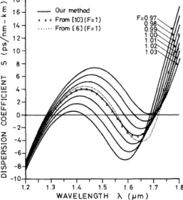
Fig. 2 shows the dispersion coefficient as a function of wavelength for various values of F . In general, there are three crossover points in the spectrum. The second zero- dispersion wavelength is very sensitive to the drawing ratio, whereas the first and the third are not. In our finite-element analysis, eleven elements result in nicely converged solution.

A

RI

R2 R3 r

Fig. 1 . Refractive-index profile of a quadruple-clad (QC) fiber.

I x x From [lOI(F=l)

1.2 1.3 1.4 1.5 1 6 1.7 1.8

WAVELENGTH h ( p m )

Fig. 2. The dispersion coefficient versus wavelength curves of the QC fiber shown in Fig. 1. The solid curves for different scale factor F are obtained by using the algorithm proposed in this paper. The crosses are the results adopted from [lo] and the dotted curve is redrawn from [6] for the F = 1 case.

The results obtained by the present algorithm (solid curves) agree in general quite well with those shown in [lo].

A more detailed comparison is made for the results with F = 1. In addition to the solid curve by the present finite- element analysis, the crosses represent the results obtained from [lo] which is based on the staircase analysis, while the dotted curve is redrawn from [6] which is based on the matrix perturbation theory. The results by the matrix perturbation theory show significant deviation as compared with those by the other two methods. The deviation may be attributed to their choice of global basis functions to expand the modal fields. The derivatives of global basis functions with respect to the radial coordinate are continuous up to arbitrary orders. However, the modal fields are in general continuous up to the first derivative only. When the index profile is discontinuous,

,

LIN er a/.: DISPERSION CHARACTERISTICS OF SINGLE-MODE OPTICAL FIBERS the modal fields have discontinuous second derivatives such that the expansion by global basis functions may be difficult. Obviously, this kind of difficulty is circumvented by using local basis functions in the present finite-element analysis.

VI. CONCLUSIONS

We have presented a new method for determining the dispersion characteristics of single-mode optical fibers with radially arbitrary refractive-index profiles. The basic features of the present method are: 1) The formulation is exact. 2 ) We can use the lower order derivatives of quantities with respect to V to calculate the higher order derivatives of w with respect to V . (3) We need only to solve one eigenvalue problem, i.e., the one for {w,

VI}.

(4) If the eigen-solution can be expressed in terms of closed-form formulas, the desired quantities may be calculated directly, as has been demonstrated for step-index fibers in Section IV. If it is not so, numerical solutions have to be resorted to. The derivative of q5 with respect to V , $, may be obtained by a few matrix manipulations. The FEM used in the numerical solution procedure has proved to be with high accuracy and offers rapid convergence speed, as can be seen from the examples in Section V. We have analyzed a type of dispersion-flattened fiber in Section V. The algorithm can be extended to the vectorial wave solution, although it is more involved.

ACKNOWLEDGMENT

The authors would like to thank Dr. I. C. Chou, Dr. K. -Y. Chen, Mr. J. Liaw, and Mr. S. -L. Tzeng of Telecommunication Laboratories for their support and useful discussions during the course of this research.

71 1

REFERENCES

B. J. Ainslie and C. R. Day, “A review of single-mode fibers with modified dispersion characteristics,” J. Lightwave Technol., vol. LT-4, T. Okoshi, Optical Fibers.

R. A. Sammut, “Analysis of approximations for the mode dispersion in monomode fiber,” Electron. Lett., vol. 15, pp. 590-591, 1979.

W. L. Mammel and L. G. Cohen, “Numerical prediction of fiber trans- mission characteristics from arbitrary refractive-index profiles,” Appl. E. K. Sharma, A. Sharma, and I. C. Goyal, “Propagation character- istics of single mode optical fibers with arbitrary index profiles: A simple numerical approach,” IEEE Quantum Electron., vol. QE-18, pp. 1484-1489, 1982.

A. Sharma and S. Banerjee, “Chromatic dispersion in single mode fiber with arbitrary index profiles: A simple method for exact numerical evaluation,” J . Lightwave Technol., vol. 7, pp. 1919-1923, 1989.

K. -J. Bathe and E. L. Wilson, Numerical Methods in Finite Element Analysis. New Jersey: Prentice-Hall, 1976.

C. R. South, “Total dispersion in step-index monomode fibres,” Electron. Lett., vol. 15, pp. 394-395, 1979.

J. W. Fleming, “Material dispersion in lightguide glasses,” Electron. Lett., vol. 14, pp. 326-328, 1978.

H. Etzkorn and W. E. Heinlein, “Low-dispersion single-mode silica fibre with undoped core and three F-doped claddings,” Electron. Lett., vol. 20, pp. 423-424, 1984.

pp. 967-979, 1986.

New York: Academic, 1982.

Opt., vol. 21, pp. 699-703, 1982.

Hoang Yen Lin, photograph and biography not available at the time of publication.

Ruey-Beei Wu, photograph and biography not available at the time of publication.

Hung-Chun Chang (S’78-M’83) photograph and biography not available at the time of publication.