基於支持向量機器方法之蛋白質β-turn預測

全文

(1)國立交通大學 National. Chiao. Tung. University. 生物資訊研究所碩士論文. 基於支持向量機器方法之蛋白質β-turn預測 Prediction of β-Turns in Proteins with Support Vector Machines. 研究生：陳孟琪指導教授：盧錦隆. 教授. 黃鎮剛. 教授. 中華民國九十四年七月.

(2) 基於支持向量機器方法之蛋白質β-turn預測 Prediction of β-Turns in Proteins with Support Vector Machines. 研究生：陳孟琪. Student：Meng-Chi Chen. 指導教授：盧錦隆. Advisor：Chin-Lung Lu Jenn-Kang Hwang. 黃鎮剛. 國立交通大學生物資訊研究所碩士論文. A Thesis Submitted to Institute of Bioinformatics College of Biological Science and Technology National Chiao Tung University in partial Fulfillment of the Requirements for the Degree of Master in Bioinformatics July 2005 Hsinchu, Taiwan, Republic of China. 中華民國九十四年七月.

(3) 基於支持向量機器方法之蛋白質β-turn預測. 學生：陳孟琪. 指導教授：盧錦隆黃鎮剛國立交通大學生物資訊研究所碩士班. 中文摘要. 本研究是利用支持向量機器的方法來預測蛋白質中β-turn的位置。在僅有蛋白質之胺基酸序列的情況下找尋有用的特徵向量，並將這些資訊輸入支持向量機器中，以此方法來預測蛋白質中哪些殘基會形成β-turn。本研究使用 426 條非同源蛋白質，做 7 倍的交叉認證以驗證預測的準確率。由結果發現除了前人研究提及的多重序列比對及二級結構資訊外，殘基暴露於溶劑的程度亦可提供有用的資訊；而胺基酸的體積及親水程度則對β-turn的預測無明顯助益。本研究整合了多重序列比對所產生的位置加權矩陣，二級結構預測資訊，以及殘基暴露於溶劑之程度的預測等三種特徵向量，則總準確率可達 79.6%，MCC值可達 0.48，皆高於其他β-turn預測方法。. i.

(4) Prediction of β-Turns in Proteins with Support Vector Machines. Student : Meng-Chi Chen. Advisor : Chin-Lung Lu Jenn-Kang Hwang. Institute of Bioinformatics National Chiao Tung University. Abstract. In this study, we use support vector machine approach to predict β-turns in protein. With only the information of protein sequence, we try to find useful feature vectors based on amino acid, and import the information to SVM to predict which residue would be in β-turn. We use 426 non-homologous proteins as dataset, and 7-folded cross validation to examine the prediction performance. In addition to multiple sequence alignment and secondary structure information, we found that relative solvent accessibility could also provide useful information in β-turn prediction. In this work, import multiple feature vectors of multiple sequence alignment information (PSSM), secondary structure prediction, and relative solvent accessibility prediction, the Qtotal could reach 79.6% and the MCC value is 0.48. Both these two measure performance are better than other previous methods. ii.

(5) 目錄中文摘要...................................................................................................................i Abstract ..........................................................................................................................ii 目錄.............................................................................................................................. iii 1. Introduction................................................................................................................1 2. Material and methods.................................................................................................5 2.1 The dataset .......................................................................................................5 2.2 Cross validation method ..................................................................................5 2.3 The support Vector Machine (SVM)................................................................6 2.4 The input feature vectors..................................................................................7 2.4.1 Sequence input vector ...........................................................................7 2.4.2 Multiple sequence alignment (PSSM) input vector ..............................7 2.4.3 Secondary structure (SS) input vector ..................................................8 2.4.4 Relative solvent accessibility (RSA) input vector ................................8 2.4.5 Chou-Fasman conformational parameter input vector .........................9 2.4.6 Amino acid solvent exposed area (SEA) input vector ........................10 2.4.7 Amino acid volume input vector.........................................................10 2.4.8 Amino acid hydropathy input vector................................................... 11 2.5 Adjusting the threshold of the output of LIBSVM ........................................ 11 2.6 Filtering.......................................................................................................... 11 2.7 Performance measures ...................................................................................12 3. Results......................................................................................................................15 3.1 Prediction accuracies of using single feature vector......................................15 3.2 Assembling feature vectors ............................................................................16 3.2.1 Prediction accuracies of using Multiple feature vectors .....................16 3.2.2 Prediction accuracies of performing Double-layer SVM ...................17 4. Discussion ................................................................................................................19 5. Reference .................................................................................................................22 Table.............................................................................................................................25 Figure ...........................................................................................................................33 Appendix......................................................................................................................38. iii.

(6) 1. Introduction The knowledge of the secondary structure of a protein has great importance in the study of the protein functionality. Currently, the main technique to determine protein structure is X-ray crystallography, which is a slow, and often a difficult process. On the other hand, the protein sequence data arising from sequencing projects is growing rapidly. Thus, it is increasingly important to predict the structure of proteins whose sequences are known. One significant step towards elucidating the structure and function of a protein is the prediction of its secondary structure. Protein secondary structure is characterized by regular elements such as α-helices and β-sheets and non-repetitive motifs such as tight turns, bulges and random coil structures. A tight turn in protein structure is defined as a site where a polypeptide chain reverses its overall direction, i.e., leads the chain to fold back on itself by nearly 180°, and the amino acid residues directly involved in forming the turn are no more than six. Depending on the number of residues forming the turn, tight turns are further classified as δ, γ, β, α, and π-turns [1]. Among the tight turns, β-turn is the most predominant one. A β-turn involves four amino acid residues. The β-turns originally recognized by Venkatachalam [2] are stabilized by a hydrogen bond between the backbone CO(i) and the backbone NH(i + 3). However, Lewis et al. [9] found that 25% of β-turns are “open,” i.e., have no intra-turn hydrogen bond at all as stipulated by Venkatachalam [2]. Open turns do not lend themselves to classification by dihedral angles. Therefore, the definition widely accepted for b-turns is: A β-turn comprises four consecutive residues where the distance between Cα(i) and Cα(i + 3) is less than 7 Å, and the tetrapeptide chain is not in a helical conformation. The distance between the Cα atoms in the first and last residues of a tetrapeptide, i.e., Cα(i) and Cα(i + 3), is a. 1.

(7) key criterion common to all β-turns, further the backbone dihedral angles in the inner residues i + 1 and i + 2 will define different types of β-turns. On average, about 25% of all protein residues comprise β-turns [5]. As one of the most common types of non-repetitive motifs in proteins, β-turns bear great significance in protein structure and function. Both from structural and functional point of view, β-turns play important biological roles as reflected from the following points: First, β-turns are four-residue reversals in proteins so that they help in the formation of higher-order structure [6]. A polypeptide chain cannot fold into a globular fold without β-turns; Second, β-turns usually occur on the exposed surface of a protein and are likely to be involved in molecular recognition processes and interactions between receptors and substrates [1; 4], and provide very useful information for designing template structures for the design of new molecules such as drugs, pesticides, and antigens. Furthermore, being at solvent-exposed surfaces, the residues that form. β-turns tend to be hydrophilic residues.; and third, also play an important role in protein folding and stability [6]. Further, one major secondary structural feature of many biologically active peptides is β-turn. β-Turn forms an integral component in the fundamental building block for anti-parallel β-sheets, which plays a good candidate for molecular recognition processes since being at solvent-exposed surfaces, and its formation is an important stage during the process of protein folding [6]. Therefore, to improve on the identification of structural motifs such as the building block for anti-parallel β-sheets and fold recognition, an accurate method to identify the location of β-turns in a protein sequence needs to be developed. Consequently, prediction of β-turns would be small step toward the overall prediction of three-dimensional structure of a protein from its amino acid sequence. It will also help in identification of structural motifs such as β-hairpin. β-turns provide very useful information for. 2.

(8) defining template structures for the design of new molecules such as drugs, pesticides, and antigens. A number of β-turn prediction methods have been developed, they can be divided into two categories: statistics-based and machine learning-based methods. The majority of statistics-based methods empirically employed the ‘positional preference approaches" [7; 8; 9; 10; 11]. In the Chou–Fasman method [8], a set of probabilities is assigned to each residue and the conformational parameters and positional frequencies are determined by calculating the relative frequency of each secondary structure. In the 1–4 and 2–3 correlation model [11], the coupling effects between the first and fourth residues and between the second and third residues are taken into account. In the sequence coupled model developed by Chou [7] within the first-order Markov chain framework, the sequence correlation effect for an entire oligo-peptide is considered. GORBTURN uses the positional frequencies and equivalent parameters [12] to remove the potential helix and strand forming residues from the β-turn prediction [13]. As to machine learning-based methods, a neural network method, BTPRED, was developed by Shepherd et al. [14] to predict the location and type of β-turns in proteins. The prediction performance could not be objectively compared because of the different dataset in these methods. Kaur and Raghava evaluated these methods and found that BTPRED was most accurate among these β-turn prediction methods [15]. BetaTPred2, an improved neural network method was developed by Kaur and Raghava [16]. In that method, they use multiple sequence alignment as input instead of the single amino acid sequence, and a great improvement in prediction performance has been achieved (Matthews correlation coefficient MCC = 0.43). k–nearest neighbor method, which is combined with a filter that uses predicted protein secondary 3.

(9) structure information was developed by Kim [17]. The SVM is an extremely successful learning theory that usually outperforms other machine learning technologies such as artificial neural networks (ANNs) and nearest neighbor methods. In recent years, SVMs have performed well in diverse applications of bioinformatics in several aspects including prediction of secondary structure [18; 19], classification of protein quaternary structure [20], etc. In this work, we attempt to predict β-turns in proteins using support vector machine (SVM) with various information derive from protein sequence, comparing with some other β-turn prediction methods that were recently evaluated by Kaur and Raghava [15], and with the other β-turn prediction methods that using the same data set. In this study. we employ a support vector machine (SVM) method to predict β-turns in proteins, and attempt to seek helpful input feature vectors only based on the information of protein sequences.. 4.

(10) 2. Material and methods 2.1 The dataset In this study, The dataset is comprised of 426 non-homologous protein chains which were first described by Guruprasad and Rajkumar [21]. This same dataset was selected by Kaur and Raghava [15] to evaluate the performance of six β-turn prediction methods. In this dataset, any two protein chains have ≦ 25% sequence identity. The structure of these proteins is determined by X-ray crystallography at better than 2.0 Å resolution, and each protein chain contains at least one β-turn . The program PROMOTIF [22] has been used to assign β-turns in proteins.. 2.2 Cross validation method A prediction method is often developed by cross-validation or jack-knife method [23]. In a full jack-knife test of N proteins, one protein is removed from the set, the training is done on the remaining N−1 proteins and the testing is done on the removed protein. This process is repeated N times by removing each protein in turn. Because of the size of the data set, the jack-knife method would be very time consuming, so a more limited cross-validation has been used. In this study, a 7-fold cross-validation technique is used where the data set is randomly divided into 7 subsets, each containing equal number of proteins. The training set is consisted of 6 subsets, and tested the prediction performance on the excluded set, the testing set. This has been done seven times to test for each subset. The final prediction results have been averaged over seven testing sets.. 5.

(11) 2.3 The support Vector Machine (SVM) The SVM is a technique of machine learning based on statistical learning theory [24]. SVM has recently be applied to solve the problems in Bioinformatics, such as secondary structure prediction [18; 19], fold recognition, etc. A library for support vector machines（LIBSVM）is used in this study [25], and which is an implementation of SVM in C language for the problem of classification, and kernel type is radial basis function. The basic idea of SVM to pattern classification can be stated briefly as follow two steps. First, map the input vectors into a feature space (often with a higher dimension), either linearly or non-linearly, which is relevant with the selection of the kernel function. Second, classifying the data by seeking an optimal separating hyperplane which can maximize the distance between two classes.（Figure 1） SVM training always seeks a global optimized solution and avoids over-fitting, so it has the ability to deal with a large number of features. A complete description of the theory of SVMs for pattern recognition has been done by Vapnik [26]. Two parameters were adjusted for optimal performance. In this work, we employed the radial basis function kernel as the kernel function. (Eq. 1) The first parameters to be determined are γ and the regularization parameter C. In the present case, we set γ=0.0625, C=2.. K(X i , X j ) = exp(-γ (X i - X j ) 2 ). 6. (1).

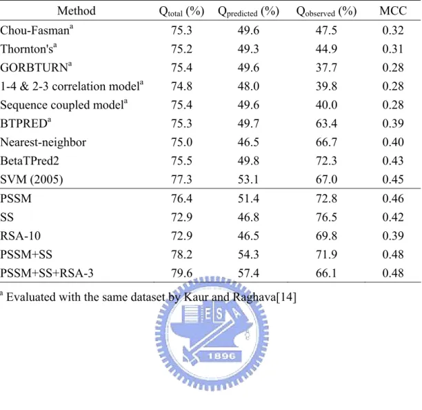
(12) 2.4 The input feature vectors Several different input feature vectors for the support vector machine（SVM） are considered. We use the classical local coding scheme of the protein sequences with a sliding window. In this study, the window size was set as 9. The “null” residue was added in order to allow a window to extend over the N- and the C-terminus.. 2.4.1 Sequence input vector The amino acid type of each residue is encoded into a 20-dimension vector consist. of. 19. “0”. and. single. “1”,. (1,0,0,0,0,0,0,0,0,0,0,0,0,0,0,0,0,0,0,0),. e.g.. alanine. glycine is. is. represented. represented. as as. (0,1,0,0,0,0,0,0,0,0,0,0,0,0,0,0,0,0,0,0), etc. The “null” residue is represented by a 20-dimension vector of all-zero.. 2.4.2 Multiple sequence alignment (PSSM) input vector With multiple sequence alignments, we use PSI-BLAST to detect distant homologues of a query sequence and generate position-specific scoring matrix (PSSM). The matrix has 21 × M elements, where M is the length of the target sequence, and each element represented the likelihood of that particular residue substitution at that position [27]. These profiles were scaled to 0-1 range using the standard logistic function: f(x) =. 1 1 + exp(-x). The “null” residue is represented by a 20-dimension vector of all-zero.. 7. (2).

(13) A figure introduce the procedure of processing PSSM input vector was shown in Figure 2.. 2.4.3 Secondary structure (SS) input vector The secondary structure of each proteins in the dataset was predicted by PSIPRED [28]. The PSIPRED prediction could output the probabilities of three states secondary structure (helix, strand, coil). Because of the value was in the range from 0-1, the three probabilities of each residue could directly be used as 3-dimension vector. The “null” residue is represented by a 3-dimension vector of all-zero. A figure introduce the procedure of processing secondary structure input vector was shown in Figure 3.. 2.4.4 Relative solvent accessibility (RSA) input vector Amino acid solvent accessibility is the degree to which a residue in a protein is accessible to a solvent molecule. Relative solvent accessibility was calculated by dividing the DSSP-defined solvent accessibility by the accessibility for a Gly-X-Gly tripeptide given by the method of Rose and Dworkin [29]. In this study, we use Jnet [30] to predict relative solvent accessibility of each residue based on a two state-model (exposed/buried) in three categories: 25%, 5%, and 0% accessible. Each residue was represented as 3-dimension vector (RSA-3) composed of zero and one, “one” means the residue was predicted as exposed at each accessible class, and “zero” means buried. The “null” residue is represented by a 3-dimension vector of all-zero. Furthermore, we use another relative solvent accessibility prediction method 8.

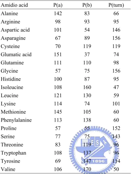
(14) developed by our lab members [36], which could predict two-state RSA in ten categories: 0-10%, 10-20%, …, 90-100%. With this RSA prediction scheme, the predicted probabilities of the ten classes were available, and they were directly be used as 10-dimension vector (RSA-10). The “null” residue is represented by a 10-dimension vector of all-zero. A figure introduce the procedure of processing RSA-10 input vector was shown in Figure 4. 2.4.5 Chou-Fasman conformational parameter input vector The Chou-Fasman algorithm for the prediction of protein secondary structure [31] is one of the most widely used predictive schemes. The Chou-Fasman method of secondary structure prediction depends on assigning a set of prediction values to a residue and then applying a simple algorithm to the conformational parameters and positional frequencies (Table 1.). The Chou-Fasman algorithm is simple in principle. The conformational parameters for each amino acid were calculated by considering the relative frequency of a given amino acid within a protein, its occurrence in a given type of secondary structure, and the fraction of residues occurring in that type of structure. These parameters are measures of a given amino acid's preference to be found in helix, sheet or coil. Using these conformational parameters, one finds nucleation sites within the sequence and extends them until a stretch of amino acids is encountered that is not disposed to occur in that type of structure or until a stretch is encountered that has a greater disposition for another type of structure. At that point, the structure is terminated. This process is repeated throughout the sequence until the entire sequence is predicted.. 9.

(15) In order to scale the conformational parameters to 0-1, each value of parameter was simply divided by 200. Each amino acid was represented as 3-dimension vector of its scaled conformational parameters. The “null” residue is represented by a 3-dimension vector of all-zero.. 2.4.6 Amino acid solvent exposed area (SEA) input vector Table 2. implies solvent accessibility information derived from Bordo and Argos [32]. The data for this table was calculated from data taken from 55 proteins in the Brookhaven data base, coming from 9 molecular families: globi ns, immunoglobins, cytochromes c, serine proteases, subtilisins, calcium binding proteins, acid proteases, toxins and virus capsid proteins. Red entries are found on the surface of a proteins on > 70% of occurrences and blue entries are found inside of a protein of < 20% of occurrences. The only clear trend in this table is that some residues, such as R and K, locate themselves so that they have access to the solvent. The hydrophobic residues, such as L and F, show no clear trend: they are found near the solvent as often as they are found buried. Each amino acid was represented as 3-dimension vector and the “null” residue is represented by a 3-dimension vector of all-zero.. 2.4.7 Amino acid volume input vector We use the amino acid volume calculated by Zamyatnin [33] as one kind of input vectors. As shown in Table 3., each amino acid was represented by its volume as one-dimension vector, and the “null” residue is represented by an one-dimension vector of zero.. 10.

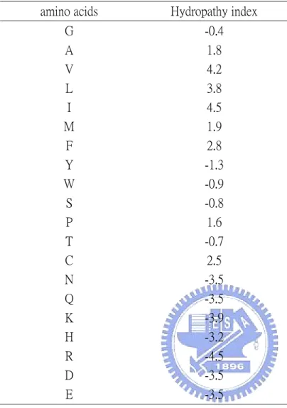
(16) 2.4.8 Amino acid hydropathy input vector Hydropathy index listed a scale combining hydrophobicity and hydorphilicity of R groups; it can be used to measure the tendency of an amino acid to seek an aqueous environment (- values) or a hydrophobic environment (+ values) [34]. As shown in Table 4., and the value was scaled to 0-1 by equation (2). Each amino acid was represented by its hydropathy as one-dimension vector. and the “null” residue is represented by an one-dimension vector of zero.. 2.5 Adjusting the threshold of the output of LIBSVM The SVM tool we used in this study (LIBSVM) could estimates the probability of each predicted class as setting parameter b as 1. In β-turn prediction, there are only two classes labels: turn and non-turn. If the probability of residues which was predicted as β-turn is more than 0.5, the output label would be β-turn, otherwise the predicted output label would be non-turn. But it seems that the threshold 0.5 is to high to get good sensitivity, so we try to lower the threshold to seek better prediction performance.. 2.6 Filtering The prediction is performed for each residue separately, since β-turns are typically multiple turns of at least four residues long, we added a simple filtering step which is similar to the “state-flipping” rule used in Shepherd et al. [14]. A set of five rules have been used in the following order:. 11.

(17) 1.. Flip isolated nonturn predictions to turn (i.e., t-t → ttt).. 2.. Flip isolated pairs of nonturn predictions to turn (i.e., t--t → tttt).. 3.. Flip isolated turn predictions to nonturn (i.e., -t- → ---).. 4.. For isolated pairs of turn predictions, flip the adjacent nonturn predictions to turn (i.e., -tt- → tttt).. 5.. For isolated triplet of turn predictions, flip the adjacent nonturn predictions to turn (i.e., -ttt- → ttttt).. 2.7 Performance measures Several parameters were widely used to measure the performance of β-turn prediction methods as described by Shepherd et al. [14], which are based on the following scalar quantities: p, the number of correctly classified β-turn residues n, the number of correctly classified non-β-turn residues o, the number non-b-turn residues incorrectly classified as β-turn (over-predictions) u, the number b-turn residues incorrectly classified as non-β-turn (under-predictions) t , the total number of residues.. 12.

(18) The parameters were described below. 1. Qtotal (or prediction accuracy), the percentage of correctly classified residues. It is the most common measure of a method’s overall performance; however, Qtotal can be misleading as β-turn residues occur much less frequently than non-β-turn residues in proteins (25 versus 75%). Therefore, one could easily achieve Qtotal = 75% merely by predicting all residues to be non-β-turn.. Q toaal =. p+n × 100 t. (3). 2. Qpredicted is the percentage of β-turn prediction that are correct, which penalizes over-predictions.. Qpredicted =. p × 100 p+o. (4). 3. Qobserved is the percentage of observed β-turns that are correctly predicted, which penalizes under-predictions.. Qobserved =. p × 100 p+u. 13. (5).

(19) 4. MCC (Matthew’s Correlation Coefficient), a single measure of performance that takes into account for both over- and under-predictions.. MCC =. pn - ou (p + o)(p + u)(n + o)(n + u). 14. (6).

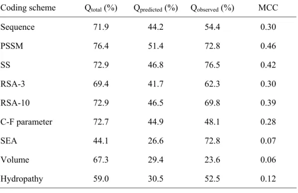
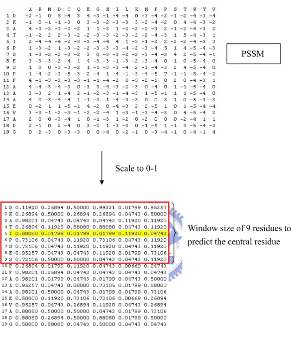
(20) 3. Results SVM is used predict the β-turns in the proteins, and it needs to import useful information. The information, which represents β-turn, is taken from a protein sequence; it can be coded through several ways and is called a feature vector.. 3.1 Prediction accuracies of using single feature vector Nine feature vector was used individually to predict β-turns in protein, and the prediction performance was listed in Table 5. As shown in Table 5., comparing the prediction performance of each input feature vector, the multiple sequence alignment feature vector which encoded PSSM as import information could achieve the best result with MCC value of 0.46 and the total accuracy (Qtotal) of 76.4. Secondary structure feature vector could also get a good prediction performance with MCC of 0.42 and Qtotal of 72.9. Both RSA-3 and RSA-10 in Table 5. mean relative solvent accessibility feature vector: RSA-3 indicates utilizing three classes of solvent accessibility prediction from Jnet; and RSA-10 denotes employing another ten-classes relative solvent accessibility prediction approach. RSA-10 shown better prediction effect than RSA-3 in all respects: Qtotal raise from 69.4% to 72.9%, Qpredicted raise from 41.7% to 46.5%, Qabserved raise from 62.3% to 69.8%, and MCC raise from 0.30 to 0.39. The predict performance of importing Chou-Fasman conformational parameter and sequence are similar. With Chou-Fasman conformational parameter feature vector, Qtotal, Qpredicted, Qobserved, and MCC are 72.7%, 44.9%, 48.1%, and 0.28 respectively. As to the performance of using sequence as input feature vector, Qtotal, Qpredicted,Qobserved, and MCC are 71.9%, 44.2%, 54.4%, and 0.30 respectively. With the solvent exposed area (SEA) feature vector, it could get a good sensitivity yielded 15.

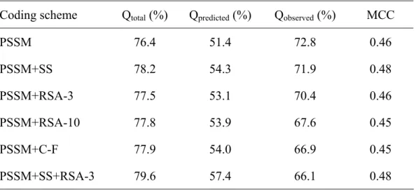
(21) Qobserved of 72.8%, which is nearly the same as the Qobserved value of multiple sequence alignment feature vector; but the correct prediction rate is much lower with the Qpredicted value of 26.6%; hence the MCC value and Qtotal are only 0.07 and 44.1% respectively. The prediction performance of SEA feature vector, volume feature vector, and hydorpathy feature vector is much lower than other feature vectors with MCC value of 0.07, 0.06, and 0.12 respectively.. 3.2 Assembling feature vectors In this study, we employ two strategies to assemble the information of each single feature vectors. One is encoding multiple feature vectors in a SVM training and testing data file; another approach is gathering the probability of being β-turn from each prediction output of single vector, and use the probabilities as import of the second layer SVM prediction.. 3.2.1 Prediction accuracies of using Multiple feature vectors As shown if Table 5., multiple sequence alignment feature vector could receive better prediction performance than other feature vectors, thus we take it as leading role, and try to join other feature vectors as import. Because of the worse prediction performance of SEA feature vector, volume feature vector, and hydorpathy feature vector, these feature vectors were not be considered in this coding scheme. The results of multiple feature vectors were listed in Table 6. In this method, all the multiple feature vectors listed in Table 6. could slightly raise Qtotal, but not every combination is fessible to improve MCC. With slightly arise. 16.

(22) Qpredicted but lower Qobserved , MCC value of PSSM+SEA-3, PSSM+SEA-10, and PSSM+C-F are the same or worse than MCC of PSSM. As to compare the prediction performance of importing two feature vectors, PSSM+SS, to single vector of PSSM, Qtotal is raise from 76.4% to 78.2%, Qpredicted is raise from 51.4% to 54.3%, and MCC value is raise from 0.46 to 0.48, but Qobserved is slightly lower from 72.8% to 71.9%. The performance of importing three feature vectors, PSSM+SS+SEA-3, is also better than single vector of PSSM, Qtotal is raise from 76.4% to 79.6%, and MCC value is raise from 0.46 to 0.48.. 3.2.2 Prediction accuracies of performing Double-layer SVM As listed in Table 5., multiple sequence alignment feature vector, secondary structure feature vector, and ten-classes relative solvent accessibility feature vector receive better prediction performance of MCC value than other single feature vectors. The probabilities of forming β-turn generated from SVM by these three feature vectors are gathered, and use as import information of the second layer SVM. The results were listed in Table 7. Comparing the performance of double-layer SVM with only use single vector, PSSM, double-layer SVM of PSSM+SS could raise Qtotal from 76.4% to 78.3%, and MCC value from 0.46 to 0.47. Besides Qobserved slightly raise from 72.8% to 74.6%, double-layer SVM of PSSM+RSA-10 and single feature vector of PSSM almost get the same result with other performance measures. Comparing the result between SS and double-layer SVM of SS+RSA-10, after including RSA information, Qtotal raise from 72.9% to 75.7%, Qpredicted rise from 46.8% to 50.3%, Qobserved decrease 76.5% to 68.4%, and the two MCC value are identical, 0.42. The predict performance between. 17.

(23) double-layer SVM of PSSM+SS and PSSM+SS+RSA-10 are similar, and both are better than only import PSSM single vector. The achievements of PSSM+SS+RSA-10 are 78.7%, 55.4%, 67.8%, 0.47 in Qtotal, Qpredicted, Qobserved, and MCC, respectively.. 18.

(24) 4. Discussion It has been shown that, as using sequence or PSI-BLAST generated position-specific scoring matrix (PSSM) to predict β-turn in proteins, including secondary structure information would improve the prediction performance [14; 15]. As shown in Table 8., in this study, even only use secondary structure information generated by PSIPRED, the prediction performance MCC could achieve 0.42, which is only lower than MCC of BetaTPred2 (0.43) [16] and SVM(2005)(0.45) [35] (both are machine learning methods with PSSM and secondary structure information as import information), but higher than any other previous methods. In this study, we found that relative solvent accessibility could provide useful information in β-turn prediction that has never been mentioned before. As only employing relative solvent accessibility as import information, the prediction performance of MCC could achieve 0.39, which is equal to MCC value of BTPRED. Although this MCC value is worse than three prediction methods, it is better than any other statistical base methods (Table 8..) As to the result of importing multiple feature vectors to SVM (Table. 6), comparing the performance between PSSM+SS+RSA-3 and PSSM+SS, while including RSA information, even though Qobserved decreased, but the increment of Qpredicted cause the raise of Qtotal. As shown in Table 5., comparing the result of two relative solvent accessibility coding scheme, the ten-classes method got better results in every performance measure than the three-classes one. Because β-turns tend to occur at solvent-exposed surface[4], it could be conjectured that the more classes in RSA prediction, the more information to represent the expose extent of a residue, and which could provide more helpful information for β-turn prediction.. 19.

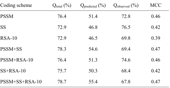
(25) Both. PSIPRED. predicted. secondary. structure. and. the. Chou-Fasmsn. conformational parameters could provide secondary structure information, but comparing with the result of these two feature vectors as listed in Table 5., the prediction performance of using Chou-Fasman parameters is worse than using PSIPRED predicted secondary structure. Maybe it is because the Chou-Fasmsn conformational parameters were calculated from specific protein set [8], it could only provide a general view of secondary structure information to each amino acid; but PSIPRED could give more limited secondary structure information in the light of specific residue. This idea could also be illustrated in comparing the result of relative solvent accessibility (RSA) with solvent exposed area (REA)(Table 8.). The solvent accessibility information used in this study was derived from Bordo and Argos [32]. The data was calculated from data taken from 55 proteins in the Brookhaven data base. In Table 2., the only clear trend is that some residues, such as R and K, locate themselves so that they have access to the solvent. The so-called hydrophobic residues, such as L and F, show no clear trend: they are found near the solvent as often as they are found buried. It also could provide a general view of the solvent exposure tendency of 20 amino acids only, but not in accordance with each residue in proteins. Thus tool-predicted RSA could provide more helpful information than SEA. Several coding scheme in this study could get better prediction performance than any other previous method. The best performance of this study is import multiple feature vectors including multiple sequence alignment feature vector, secondary structure feature vector, and relative solvent accessibility feature vector (three classes). This approach yields superior results compared with existing method on the same dataset (Table 8.). Comparing the four performance measures with SVM(2005), only Qobserved has almost the same value, other measures receive better result in this study:. 20.

(26) Qtotal, Qpredicted, Qobserved, and MCC are 79.6%, 57.4%, 66.1%, and 0.48 respectively in this work; and 77.3%, 53.1%, 67.0%, and 0.45 respectively in SVM(2005). In conclusion, the β-turn prediction method described here yields predictions that are significantly more accurate than previous methods. Not only multiple sequence alignment and secondary structure information are important, relative solvent accessibility could also assist the prediction of β-turns.. 21.

(27) 5. Reference 1. 2.. 3. 4. 5.. 6.. 7. 8.. 9. 10. 11. 12.. 13. 14.. 15.. Chou, K. C. (2000). Prediction of tight turns and their types in proteins. Anal Biochem. 286, 1-16. Venkatachalam, C. M. (1968) Stereo chemical criteria for polypeptides and proteins. V. Conformation of a system of three linked peptide units. Biopolymers 6, 1425–1436. Richardson, J. S. (1981). The anatomy and taxonomy of protein structure. Adv Protein Chem. 34, 167-339. Rose, G. D., Gierasch, L. M. & Smith, J. A. (1985). Turns in peptides and proteins. Adv Protein Chem. 37, 100-109. Kabsch, W. & Sander, C. (1983). Dictionary of protein secondary structure: pattern recognition of hydrogen-bonded and geometrical features. Biopolymers 22, 2577-2637. Takano, K., Yamagata, Y. & Yutani, K. (2000). Role of amino acid residues at turns in the conformational stability and folding of human lysozyme. Biochemistry 39, 8655-8665. Chou, K. C. & Blinn, J. R. (1997). Classification and prediction of beta-turn types. J Protein Chem. 16, 575-595. Chou, P. Y. & Fasman, G. D. (1974). Conformational parameters for amino acids in helical, beta-sheet, and random coil regions calculated from proteins. Biochemistry 13, 211-222. Lewis, P. N., Momany, F. A. & Scheraga, H. A. (1973). Chain reversals in proteins. Biochim Biophys Acta. 303, 211-229. Wilmot, C. M. & Thornton, J. M. (1988). Analysis and prediction of the different types of beta-turn in proteins. J Mol Biol. 203, 221-232. Zhang, C. T. & Chou, K. C. (1997). Prediction of β-turns in proteins by 1-4 & 2-3 Correlation Model. Biopolymers 41, 673-702. Gibrat, J. F., Garnier, J. & Robson, B. (1987). Further developments of protein secondary structure prediction using information theory. New parameters and consideration of residue pairs. J Mol Biol 198, 425-443. Wilmot, C. M. & Thornton, J. M. (1990). Beta-turns and their distortions: a proposed new nomenclature. Protein Eng 3, 479-493. Shepherd, A. J., Gorse, D. & Thornton, J. M. (1999). Prediction of the location and type of beta-turns in proteins using neural networks. Protein Sci 8, 1045-55. Kaur, H. & Raghava, G. P. (2002). An evaluation of beta-turn prediction methods. Bioinformatics 18, 1508-14. 22.

(28) 16. 17. 18. 19.. 20.. 21.. 22. 23. 24. 25. 26. 27.. 28. 29.. 30.. 31. 32.. Kaur, H. & Raghava, G. P. (2003). Prediction of beta-turns in proteins from multiple alignment using neural network. Protein Sci 12, 627-34. Kim, S. (2004). Protein beta-turn prediction using nearest-neighbor method. Bioinformatics 20, 40-44. Ward, J. J., McGuffin, L. J., Buxton, B. F. & Jones, D. T. (2003). Secondary structure prediction with support vector machines. Bioinformatics 19, 1650-5. Guo, J., Chen, H., Sun, Z. & Lin, Y. (2004). A novel method for protein secondary structure prediction using dual-layer SVM and profiles. Proteins 54, 738-43. Zhang, S. W., Pan, Q., Zhang, H. C., Zhang, Y. L. & Wang, H. Y. (2003). Classification of protein quaternary structure with support vector machine. Bioinformatics 19, 2390-6. Guruprasad, K. & Rajkumar, S. (2000). Beta-and gamma-turns in proteins revisited: a new set of amino acid turn-type dependent positional preferences and potentials. J Biosci 25, 143-56. Hutchinson, E. G. & Thornton, J. M. (1996). PROMOTIF--a program to identify and analyze structural motifs in proteins. Protein Sci 5, 212-20. Chou, K. C. & Zhang, C. T. (1995). Prediction of protein structural classes. Crit Rev Biochem Mol Biol 30, 275-349. Cortes, C. & Vapnik, V. (1995). Support vector networks. Machine Learning 20, 273-293. Chang, C. C. & Lin, C. J. (2001). LIBSVM: a library for support vector machines. Software available from http://www.csie.ntu.edu.tw/~cjlin/libsvm. Vapnik, V. (1998). Statistical Learning Theory Wiley N.Y. Altschul, S. F., Madden, T. L., Schaffer, A. A., Zhang, J., Zhang, Z., Miller, W. & Lipman, D. J. (1997). Gapped BLAST and PSI-BLAST: a new generation of protein database search programs. Nucleic Acids Res 25, 3389-402. Jones, D. T. (1999). Protein secondary structure prediction based on position-specific scoring matrices. J Mol Biol 292, 195-202. Rose, G. D. & Dworkin, J. E. (1989). The hydrophobicity profile. In: Fasman GD, editor. Prediction of protein structure and the principles of protein conformation 625-634. New York: Plenum Press, NY, 10013. Cuff, J. A. & Barton, G. J. (2000). Application of multiple sequence alignment profiles to improve protein secondary structure prediction. Proteins 40, 502-11. Chou, P. Y. & Fasman, G. D. (1977). Beta-turns in proteins. J Mol Biol 115, 135-75. Bordo, D. & Argos, P. (1991). Suggestions for "safe" residue substitutions in 23.

(29) 33. 34. 35. 36.. site-directed mutagenesis. J Mol Biol 217, 721-9. Zamyatnin, A. A. (1972). Protein volume in solution. Prog Biophys Mol Biol 24, 107-23. Kyte, J. & Doolittle, R. F. (1982). A simple method for displaying the hydropathic character of a protein. J Mol Biol 157, 105-32. Zhang, Q., Yoon, S. & Welsh, W. J. (2005). Improved method for predicting beta-turn using support vector machine. Bioinformatics 21, 2370-4. 徐蔚倫，「從蛋白質序列預測殘基相對溶劑可接觸性」，國立交通大學，碩士論文，民國 94 年。. 24.

(30) Table 1. Chou-Fasman conformational parameters Amidio acid. P(a). P(b). P(turn). Alanine. 142. 83. 66. Arginine Aspartic acid Asparagine Cysteine Glumatic acid Glutamine Glycine Histidine Isoleucine Leucine Lysine Methionine Phenylalanine Proline Serine Threonine Tryptophan Tyrosine Valine. 98 101 67 70 151 111 57 100 108 121 114 145 113 57 77 83 108 69 106. 93 54 89 119 37 110 75 87 160 130 74 105 138 55 75 119 137 147 170. 95 146 156 119 74 98 156 95 47 59 101 60 60 152 143 96 96 114 50. P(a), P(b) and P(turn) are conformational parameters of helix, β-sheet and β-turns.. 25.

(31) Table 2. Solvent exposed area (SEA) of amino acids Amino acid Serine Threonine Alanine Glycine Proline Cysteine Aspartic acid Glumatic acid Glutamine Asparagine Leucine Isoleucine Valine Methionine Phenylalanine Tyrosine Tryptophan Lysine Arginine Histidine. SEA > 30 Å2. SEA < 10 Å2. 30 > SEA > 10 Å2. 0.7 0.71 0.48 0.51 0.78 0.32 0.81 0.93 0.81 0.82 0.41 0.39 0.4 0.44 0.42 0.67 0.49 0.93 0.84 0.66. 0.2 0.16 0.35 0.36 0.13 0.54 0.09 0.04 0.1 0.1 0.49 0.47 0.5 0.2 0.42 0.2 0.44 0.02 0.05 0.19. 0.1 0.13 0.17 0.13 0.09 0.14 0.1 0.03 0.09 0.08 0.1 0.14 0.1 0.36 0.16 0.13 0.07 0.05 0.11 0.15. 26.

(32) Table 3. volume and hydropathy index of amino acids amino acids. volume. G. 60.1. A V L I M F Y W S P T. 88.6 140 166.7 166.7 162.9 189.9 193.6 227.8 89 112.7 116.1. C N Q K H R D E. 108.5 114.1 143.8 168.6 153.2 173.4 111.1 138.4. 27.

(33) Table 4. hydropathy index of amino acids amino acids. Hydropathy index. G. -0.4. A V L I M F Y W S P T. 1.8 4.2 3.8 4.5 1.9 2.8 -1.3 -0.9 -0.8 1.6 -0.7. C N Q K H R D E. 2.5 -3.5 -3.5 -3.9 -3.2 -4.5 -3.5 -3.5. 28.

(34) Table 5. The prediction performance based on single feature vector Coding scheme. Qtotal (%). Qpredicted (%). Qobserved (%). MCC. Sequence. 71.9. 44.2. 54.4. 0.30. PSSM. 76.4. 51.4. 72.8. 0.46. SS. 72.9. 46.8. 76.5. 0.42. RSA-3. 69.4. 41.7. 62.3. 0.30. RSA-10. 72.9. 46.5. 69.8. 0.39. C-F parameter. 72.7. 44.9. 48.1. 0.28. SEA. 44.1. 26.6. 72.8. 0.07. Volume. 67.3. 29.4. 23.6. 0.06. Hydropathy. 59.0. 30.5. 52.5. 0.12. 29.

(35) Table 6. The prediction performance based on multiple feature vector Coding scheme. Qtotal (%). Qpredicted (%). Qobserved (%). MCC. PSSM. 76.4. 51.4. 72.8. 0.46. PSSM+SS. 78.2. 54.3. 71.9. 0.48. PSSM+RSA-3. 77.5. 53.1. 70.4. 0.46. PSSM+RSA-10. 77.8. 53.9. 67.6. 0.45. PSSM+C-F. 77.9. 54.0. 66.9. 0.45. PSSM+SS+RSA-3. 79.6. 57.4. 66.1. 0.48. 30.

(36) Table 7. The prediction performance based on multiple feature vector Coding scheme. Qtotal (%). Qpredicted (%). Qobserved (%). MCC. PSSM. 76.4. 51.4. 72.8. 0.46. SS. 72.9. 46.8. 76.5. 0.42. RSA-10. 72.9. 46.5. 69.8. 0.39. PSSM+SS. 78.3. 54.6. 69.4. 0.47. PSSM+RSA-10. 76.4. 51.3. 74.6. 0.46. SS+RSA-10. 75.7. 50.3. 68.4. 0.42. PSSM+SS+RSA-10. 78.7. 55.4. 67.8. 0.47. 31.

(37) Table 8. Comparing the prediction performance with previous methods Method. Qtotal (%). Qpredicted (%). Qobserved (%). MCC. Chou-Fasman Thornton'sa GORBTURNa 1-4 & 2-3 correlation modela Sequence coupled modela BTPREDa Nearest-neighbor BetaTPred2 SVM (2005). 75.3 75.2 75.4 74.8 75.4 75.3 75.0 75.5 77.3. 49.6 49.3 49.6 48.0 49.6 49.7 46.5 49.8 53.1. 47.5 44.9 37.7 39.8 40.0 63.4 66.7 72.3 67.0. 0.32 0.31 0.28 0.28 0.28 0.39 0.40 0.43 0.45. PSSM. 76.4. 51.4. 72.8. 0.46. SS. 72.9. 46.8. 76.5. 0.42. RSA-10 PSSM+SS PSSM+SS+RSA-3. 72.9 78.2 79.6. 46.5 54.3 57.4. 69.8 71.9 66.1. 0.39 0.48 0.48. a. a. Evaluated with the same dataset by Kaur and Raghava[14]. 32.

(38) Figure 1. Optimal separating hyperplane(OSH) of SVM. 33.

(39) PSSM. Scale to 0-1. Window size of 9 residues to predict the central residue. Figure 2. The procedure of processing PSSM input vector. 34.

(40) Window size of 9 residues to predict the central residue. Figure 3. The procedure of processing secondary structure input vector. 35.

(41) Window size of 9 residues to predict the central residue. Figure 4. The procedure of processing RSA-10 input vector. 36.

(42) Sequences. Transform to input feature vectors. SVM classifier. Adjust the threshold of output probability. Filtering. Final result. Figure 5. Simple flow chart of prediction β-turns using SVM in this study. 37.

(43) Appendix 1. Types of β-turns. * Chou, K. C. (2000). Prediction of tight turns and their types in proteins. Anal Biochem. 286, 1-16. (55) Hutchinson, E. G., and Thornton, J. M. (1994) A revised set of potentials for β-turn formation in proteins. Protein Sci. 3, 2207– 2216.. 38.

(44) Appendix 1. (Continued). 39.

(45) 40.

(46) * Chou, K. C. (2000). Prediction of tight turns and their types in proteins. Anal Biochem. 286, 1-16. 41.

(47) Appendix 2. Protein chains (426) from Protein Data Bank used for β-turns analysis 119l 1a2zA 1a8i 1afwA 1ajsA 1alu 1anf 1apyB 1at0 1ayl 1benB 1bkrA 1cbn 1chmA 1cseI 1dokA 1ecl 1ezm 1fua 1garA 1gotG 1hfc 1idaA 1isuA 1kid 1kvu 1lit 1lucB 1mpgA 1mtyD 1nbaB 1nox 1onc 1oyc 1php 1poc. 153l 1a34A 1a9s 1agjA 1ak0 1alvA 1aocA 1aq0A 1atlA 1azo 1bfd 1brt 1cem 1ckaA 1csh 1dorA 1ecpA 1fdr 1furA 1gd1O 1gsa 1hgxA 1idk 1ixh 1knb 1kwaB 1lki 1mai 1mrj 1mtyG 1nbcA 1np1A 1onrA 1pcfA 1pii 1pot. 1a1iA 1a62 1aac 1agqD 1ak1 1aly 1aohA 1aq6A 1atzB 1ba1 1bfg 1btkB 1ceo 1clc 1csn 1dosA 1ede 1fds 1fus 1gdoA 1guqA 1hoe 1ido 1jdw 1kpf 1lam 1lkkA 1mbd 1mrp 1mucA 1nciB 1npk 1opd 1pda 1plc 1ppn. 1a1x 1a68 1aba 1ah7 1ako 1amm 1aol 1aqb 1avmA 1bbpA 1bftA 1btn 1cewI 1cnv 1ctj 1dun 1edg 1fit 1fvkA 1gifA 1gvp 1hsbA 1ifc 1jer 1kptA 1latB 1lmb3 1mkaA 1msc 1mugA 1neu 1nulB 1opy 1pdo 1pmi 1ppt 42. 1a28B 1a6q 1ad2 1aho 1akz 1amp 1aop 1aqzB 1awd 1bdmB 1bgc 1bv1 1cex 1cpcB 1cydA 1dupA 1edmB 1fleI 1fwcA 1gky 1ha1 1htrP 1igd 1jetA 1kuh 1lbu 1lml 1mldA 1msi 1mwe 1nfn 1nwpA 1orc 1pgs 1pne 1prxB. 1a2pA 1a7tA 1adoA 1aj2 1al3 1amuA 1aoqA 1arb 1awsA 1bdo 1bgp 1byb 1cfb 1cpo 1dad 1dxy 1edt 1fmtB 1g3p 1gnd 1havA 1hxn 1iibA 1jfrA 1kveA 1lcl 1lt5D 1mml 1msk 1mzm 1nif 1nxb 1ospO 1phe 1pnkB 1ptq. 1a2yA 1a8e 1af7 1ajj 1alo 1amx 1aozA 1arv 1axn 1bebA 1bkf 1c52 1chd 1cseE 1dkzA 1eca 1erv 1fna 1gai 1gotB 1hcrA 1iakA 1iso 1jpc 1kveB 1lis 1ltsA 1molA 1mtyB 1nar 1nls 1ois 1ovaA 1phnA 1poa 1pty.

(48) 1pud 1regY 1rss 1rypJ 1sluA 1tadC 1tml 1uch 1vhh 1vsd 1who 1xsoA 1yveI 2ayh. 1qba 1reqD 1rsy 1sbp 1smd 1tca 1trkA 1unkA 1vid 1vwlB 1whtB 1xyzA 1zin 2baa. 1qnf 1rgeA 1rvaA 1sfp 1spuA 1tfe 1tsp 1urnA 1vif 1wab 1wpoB 1yaiC 256bA 2bbkH. 1r69 1rhs 1ryp1 1sftB 1sra 1thv 1tvxA 1uxy 1vin 1wba 1xgsA 1yasA 2a0b 2bbkL. 1ra9 1rie 1ryp2 1sgpI 1stmA 1thx 1tys 1v39 1vjs 1wdcA 1xikA 1ycc 2abk 2bopA. 1rcf 1rmg 1rypF 1skz 1svb 1tib 1uae 1vcaA 1vls 1wer 1xjo 1yer 2acy 2cba. 1rec 1rro 1rypI 1sltA 1svpA 1tif 1ubi 1vcc 1vpsA 1whi 1xnb 1ytbA 2arcA 2ccyA. 2chsA 2fdn 2hpdA 2mcm 2plc 2scpA 2vhbB 3daaA 3seb 5csmA 6gsvA. 2ctc 2fha 2hts 2msbB 2por 2sicI 2wea 3grs 3tss 5hpgA 7ahlA. 2cyp 2fivA 2i1b 2nacA 2pspA 2sil 3b5c 3lzt 3vub 5icb 7rsa. 2dri 2gdm 2ilk 2pgd 2pth 2sn3 3chy 3nul 4bcl 5p21 8abp. 2end 2hbg 2kinA 2phy 2rn2 2sns 3cla 3pcgM 4mt2 5pti 8rucI. 2eng 2hft 2kinB 2pia 2rspB 2tgi 3cox 3pte 4pgaA 5ptp 8rxnA. 2erl 2hmzA 2lbd 2pii 2sak 2tysA 3cyr 3sdhA 4xis 6cel. 43.

(49)