Publisher: Taylor & Francis
Informa Ltd Registered in England and Wales Registered Number: 1072954 Registered office: Mortimer House, 37-41 Mortimer Street, London W1T 3JH, UK
Journal of the Chinese Institute of Engineers
Publication details, including instructions for authors and subscription information: http://www.tandfonline.com/loi/tcie20
A new model and heuristic algorithms for the
multiple
‐depot vehicle scheduling problem
Jin‐Yuan Wang a & Chih‐Kang Lin b
a
Department of Transportation Technology and Management , National Chiao Tung University , Hsinchu, 300, Taiwan, R.O.C. Phone: 886–3–5131336 Fax: 886–3–5131336 E-mail:
b
Department of Transportation Technology and Management , National Chiao Tung University , Hsinchu, 300, Taiwan, R.O.C.
Published online: 04 Mar 2011.
To cite this article: Jin‐Yuan Wang & Chih‐Kang Lin (2010) A new model and heuristic algorithms for the multiple‐depot vehicle scheduling problem, Journal of the Chinese Institute of Engineers, 33:2, 287-299
To link to this article: http://dx.doi.org/10.1080/02533839.2010.9671618
PLEASE SCROLL DOWN FOR ARTICLE
Taylor & Francis makes every effort to ensure the accuracy of all the information (the “Content”) contained in the publications on our platform. However, Taylor & Francis, our agents, and our licensors make no
representations or warranties whatsoever as to the accuracy, completeness, or suitability for any purpose of the Content. Any opinions and views expressed in this publication are the opinions and views of the authors, and are not the views of or endorsed by Taylor & Francis. The accuracy of the Content should not be relied upon and should be independently verified with primary sources of information. Taylor and Francis shall not be liable for any losses, actions, claims, proceedings, demands, costs, expenses, damages, and other liabilities whatsoever or howsoever caused arising directly or indirectly in connection with, in relation to or arising out of the use of the Content.
This article may be used for research, teaching, and private study purposes. Any substantial or systematic reproduction, redistribution, reselling, loan, sub-licensing, systematic supply, or distribution in any
form to anyone is expressly forbidden. Terms & Conditions of access and use can be found at http:// www.tandfonline.com/page/terms-and-conditions
A NEW MODEL AND HEURISTIC ALGORITHMS FOR THE
MULTIPLE-DEPOT VEHICLE SCHEDULING PROBLEM
Jin-Yuan Wang and Chih-Kang Lin*
ABSTRACT
The multiple-depot vehicle scheduling problem (MDVSP) addresses the work of assigning vehicles to serve a given set of time trips with the consideration of certain requirements representing the market rules. Extensive studies in the literature ad-dress the MDVSP, but because of the complexity of the problem, the findings of those researchers are still not enough to represent real world situations in Taiwan. Formu-lation for the MDVSP typically contains the following assumptions: (1) the size of fleet or maximum number of available vehicles at each depot is known already, (2) all trip serving costs are usually simplified as a single term in the objective function, which fails to reflect public transit operator concerns, (3) the applied deadheading strategy is static less flexibility, (4) there is no discussion of differences of route change frequency in the problem. This paper presents a new MDVSP model to ad-dress the above issues. A greedy heuristic algorithm based on the divide-and-conquer technique is also proposed to solve the MDVSP effectively. Computational tests are performed on the Kinmen Bus Administration (KBA) and results demonstrate that the proposed new model and the greedy heuristic algorithm for the MDVSP are effective in solving real world problems.
Key Words: transportation, multiple-depot vehicle scheduling problem (MDVSP),
heuristic, greedy algorithm.
*Corresponding author. (Tel: 5131336; Fax: 886-3-5725804; Email: [email protected])
The authors are with the Department of Transportation Technology and Management, National Chiao Tung University, Hsinchu 300, Taiwan, R.O.C.
I. INTRODUCTION
Vehicle scheduling is one of the most important transportation industry jobs, especially for public transit services. This problem addresses the work of assigning vehicles to serve a given set of time trips, considering certain market rule requirements. An optimal schedule generally satisfies minimum fleet size of vehicles and minimum operational costs in-cluding costs for vehicle idle time at depots and the number of deadhead trips. Extensive studies in the literature address the multiple-depot vehicle sched-uling problem (MDVSP). Bodin and Golden (1983) (1981), and Ball et al. (1995) point out some critical requirements for this problem formulation, such as vehicle idle time, number of depots, fleet size, and
deadhead trips. Minimizing the number of required vehicles and operational costs which combine vehicle idle time and deadhead trip costs are the main com-ponents in the MDVSP objective function. Previous studies propose some approximate exact solution al-gorithms to deal with the MDVSP. Those efforts help efficiently solve the MDVSP and obtain a reasonable answer. Studies by Carraresi and Gallo (1983), Carpaneto et al. (1989), Mesquita and Paixão (1990), Lamatsch (1992), Forbes et al. (1994), Ribeiro and Soumis (1994), Beasley and Cao (1996), Kokott and Löbel (1996), Löbel (1997), Haghni et al. (2002), Haghani and Banihashemi (2003), Gintner et al. (2005), Pepin et al. (2006), Kliewer et al. (2006) and Hadjar et al. (2006) also show these efforts.
The assumptions mentioned above however, are still not enough to represent real world situations in Taiwan (Wang and Lin, 2003). Formulation for the MDVSP typically contains the following assumptions: (1) the size of fleet or maximum number of available vehicles at each depot is known already, (2) all trip serving costs are usually simplified as a single term
in the objective function, which fails to reflect pub-lic transit operator concerns, (3) sufficient flexibility for adopting different deadheading strategies in for-mulation is not provided, (4) there is no discussion of different route change frequencies in the problem. These assumptions leave significant limitations while applying the MDVSP to solve real world problems, especially for public transit.
Operators are usually troubled in deciding the number of available vehicles at each depot in practice. In particular, assigning too many vehicles to one de-pot can cause vehicle shortages at other dede-pots. Moreover, finding a good solution is crucial for the Taiwan public transit industry, since prices are gen-erally kept low for the public welfare. As a result, most Taiwan public transit operators focus on reduc-ing vehicle fleet size as much as possible even in the schedule planning stage. Some studies (Bodin and Golden, 1981; Carraresi and Gallo, 1983; Ball et al., 1995) argue that it is not necessary to minimize the number of required vehicles since it is not a short term planning concern. Extra vehicles, if they do exist, can be used for other profit-making activities such as chartering, if required vehicles are kept to a minimum. Different types of costs need to be considered separately in order to address different decision makers’ preferences. Considering public transit operation needs in terms of cost, one should represent more than one perspective. Most researchers use only a single de-terministic term to present the concept of cost accom-modated in the objective function, which is not a problem from a mathematical point of view. However, it could be a problem for the decision maker of public transit operation by this approach, since it is not easy to in-tegrate different types of cost into a single one.
Deadhead trip arrangement is a common trade off influencing operating efficiency. Most research-ers base model formulation on a pre-determined network. Associated deadhead arcs and costs are added to the network if deadhead trips are allowed. Again, this is perfectly suitable from the theoretical point of view. However, public transit operators in the real world might want to try adopting different deadhead strategies before making decisions. It is a flexible way to incorporate the deadhead trip consideration into the model formulation, as constraint functions.
Changing service routes is not considered a good public transit practice. Real world drivers are usu-ally assigned to a specific vehicle route they are fa-miliar with. A vehicle assigned to serve more routes requires a driver familiar with all those routes. Most operators agree that keeping route change frequency as low as possible is important (Wang and Lin, 2006). Most studies, unfortunately, seem to ignore this issue. Literature findings show that the computation capability of existing optimization technologies for
solving the MDVSP are limited according to the prob-lem size (i.e. number of trips) since it is character-ized as NP-hard (Bertossi et al., 1987). Finding the optimal solution within an acceptable time is a prob-lem when exceeding 850 trips for the MDVSP (Hadjar et al., 2006). For handling large scale MDVSPs, there are some applied techniques such as the column gen-eration algorithm (Ribeiro and Soumis, 1994; Löbel, 1997), the Lagrangian relaxation algorithm (Mesquita and Paixão, 1990; Lamatsch, 1992; Kokott and Löbel, 1996), metaheuristics algorithms: the Tabu search al-gorithm (Cordeau et al., 2001; Pepin et al., 2006), Genetic Algorithms (Su and Yu, 2006), and many other proposed heuristic algorithms: an auction algorithm for the quasi- assignment formulation (Freling, 1997), a schedule first-cluster second approach (Daduna and Paixão, 1995) and a cluster first-schedule second ap-proach (Carraresi and Gallo, 1983) can be found in related studies. Most of these algorithms solve the MDVSP efficiently and effectively with the prereq-uisite of having a particular network structure to ease the solution process (Pepin et al., 2006). However, time-consuming network constructions are not accept-able in real world public transit operations. Therefore, solving large scale MDVSPs efficiently and effectively remains a challenge. It also determines whether or not the identified solutions can be applied in real world operations. This is particularly true for transit op-erations that require quick responses.
This paper proposes a new MDVSP model with the objectives of minimizing vehicle idle time, mini-mizing fleet size, minimini-mizing service route change frequency, and deadhead trip strategy concerns. This study also presents a heuristic solution procedure by dividing the MDVSP into relatively easy problems to solve this model efficiently and effectively. The rest of the paper is organized as follows: This work first introduces a new MDVSP model formulation, and then illustrates a greedy algorithm for solving the MDVSP formulation. Finally, a real case in Taiwan is adopted to show the efficiency and effectiveness of the theoretical approach in this study.
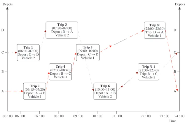
II. A NEW MDVSP MODEL FORMULATION 1. The Basic Assumptions Made for the MDVSP Figure 1 graphically illustrates the MDVSP. The horizontal and vertical axes represent time span and depot locations respectively. N trips have to be per-formed by a minimal number of vehicles daily. Each box represents a single trip, which includes service duration, departure depot, arrival depot, and service vehicle index. The arc, connecting two boxes, indi-cates the sequence of trips served by a vehicle. Each block includes trips that satisfy constraints and can
be served by one vehicle, and each vehicle must re-turn to the same depot from where it departs. Blocks in the MDVSP are acyclic, i.e. there are no cycles in the block, because of the time dimension. A number of basic assumptions for this MDVSP made by this study are listed below.
(1) Each trip must be served by one and only one vehicle;
(2) All trips need to be served by a minimal number of vehicles;
(3) The following attributes of each trip are known. That is, each trip i is associated with the informa-tion of departure depot, arrival depot, departure time, length of service time (or duration), specific route number, and cost of serving the trip; (4) Different types of deadhead trip (to be discussed
later) are allowed;
(5) For any feasible solution, the costs of perform-ing all trips (
Σ
Ni = 1oci) are the same, so this costcan be ignored.
The MDVSP is defined formally as: where N = {1, 2, ..., n} represents the known trip set, and I de-notes the feasible set of pairs of trips, each pair is connected by an arc. With each depot p ∈ P, this formulation associates the graph Gp = (Vp, Ap), where
n + p denotes the pth depot, Vp = N ∪ {n + p}, and Ap
= I ∪ {n + p} × N) ∪ (N ×{ n + p}). The arc cost cij,
(i, j) ∈ Ap, is independent of p if (i, j) ∈ I, while
cn + p, j for j ∈ N, and ci, n + p for i ∈ N, which depends
on p. xpij is the flow for type p through arc (i, j) ∈ Ap.
2. Model Formulation
According to the notations of graph theory men-tioned above, the proposed mathematical formulation for the MDVSP used in this study is introduced as follows.
Minimize α( cijxij p
Σ
i, j∈ NΣ
p∈ P ) +β (Σ
xn + p, jp j∈ NΣ
p∈ P + xj, n + p pΣ
j∈ N ) +λ( ( (γγj–γi j+γi) xijpΣ
i, j∈ NΣ
p∈ P ) +ω ( ξijxij pΣ
i, j∈ NΣ
p∈ P + ξj, n + pxj, n + p pΣ
j∈ N + ξn + p, jxn + p, j pΣ
j∈ N ) (1) s.t. xij pΣ
i∈ N + xn + p, j p = xji p + xj, n + p pΣ
i∈ N ∀p ∈ P ∀j ∈ N (2) ( xij pΣ
j∈ N + xi, n + p p )Σ
p∈ P = 1 ∀i ∈ N (3) ( p – si)xn + p, ipΣ
i∈ N ≤ 0 ∀p ∈ P (4) ( p – ej)xj, n + p pΣ
j∈ N ≤ 0 ∀p ∈ P (5) (ei– sj)xijpΣ
p∈ P ≤ 0 ∀(i, j) ∈ I (6) Trip 3 (07:20~09:00) Depot : D → A Vehicle 2 Trip 1 (06:00~07:00) Depot : C → D Vehicle 2 Trip 2 (06:15~07:20) Depot : A → B Vehicle 1 Trip 5 (09:00~10:00) Depot : C → D Vehicle 1 Trip 6 (10:00~11:00) Depot : A → B Vehicle 2 Trip N-1 (21:30~22:40) Trip: B → C Vehicle 2 Trip N (22:00~23:30) Trip: D → A Vehicle 1 Trip 4 (07:30~08:40) Depot : B → C Vehicle 1 D Depots Depots 06 : 00 00 : 00 07 : 00 08 : 00 09 : 00 10 : 00 11 : 00 22 : 00 23 : 00 24 : 00 Time C B A D C B AFig. 1 Daily operation diagram for multiple depot vehicle scheduling
xpij∈ {0, 1} ∀p ∈ P (7)
xijp=
1 if trips i and j are served consecutively by avehicle from depot p
0 otherwise ;
The objective function (Eq. (1)) can be decom-posed into four parts, seeking to minimize total costs. Its logical meaning can be described as follows.
The first part (α(
Σ
cijxijp i, j∈ NΣ
p∈ P )) of Eq. (1)
represents the summation of total vehicle idle time cost, since extra idle time at depots usually increases personnel cost or makes the crew scheduling prob-lem more difficult (Baita et al., 2000). The cost of vehicle idle time can be measured based on the pay rate (dollars/min) for a hired driver, represented in the model as parameter α. The second part (β ( xn + p, j p
Σ
j∈ NΣ
p∈ P + xj, n + p pΣ
j∈ N )) of Eq. (1) represents the total cost of vehicle depreciation, measured based on its purchase cost and its reasonable lifetime. The third part (λ( ( γj–γi (γj+γi) xijp)Σ
i, j∈ NΣ
p∈ P ) of Eq. (1)repre-sents the total routes changing time with the best arrangement. Parameter λ represents the penalty for every route change. For any two trips i, j, γi and γj
representing the specific route numbers respectively, they are compatible when serving trip j immediately after trip i using the same vehicle. If γi≠ γj, the value
of the the ceiling function ( (γγj–γi j+γi)
) is one, which represents one route-change per block, and the cost value of λ increases in the objective function. On
the contrary, if γi = γj, the value of the ceiling
func-tion ( (γγj–γi j+γi)
) is zero, which means there is no pen-alty to the objective function value. The last part (ω
Σ
p∈ P .( ξ ijxij p
Σ
i, j∈ N + ξj, n + pxj, n + p pΣ
j∈ N + ξn + p, jxn + p, j pΣ
j∈ N ))of Eq. (1) represents the total cost of performing dead-head trips. This formulation allows deaddead-head trips between different depots if the arrival terminal of trip i and the departure terminal of trip j are not the same when these two trips i, j are compatible. Based on this definition, this part of the objective function con-sists of three items: the weighted cost for deadhead trips occurring from depots to departure terminal of trips, between the departure and arrival terminals of any trips, and from departure terminal of trips to all depots. While deadhead trips take place in all blocks in the situation described above, the cost of ω × ξij
increases in the objective function. These four parts of Eq. (1) are commonly used in solving vehicle scheduling problems.
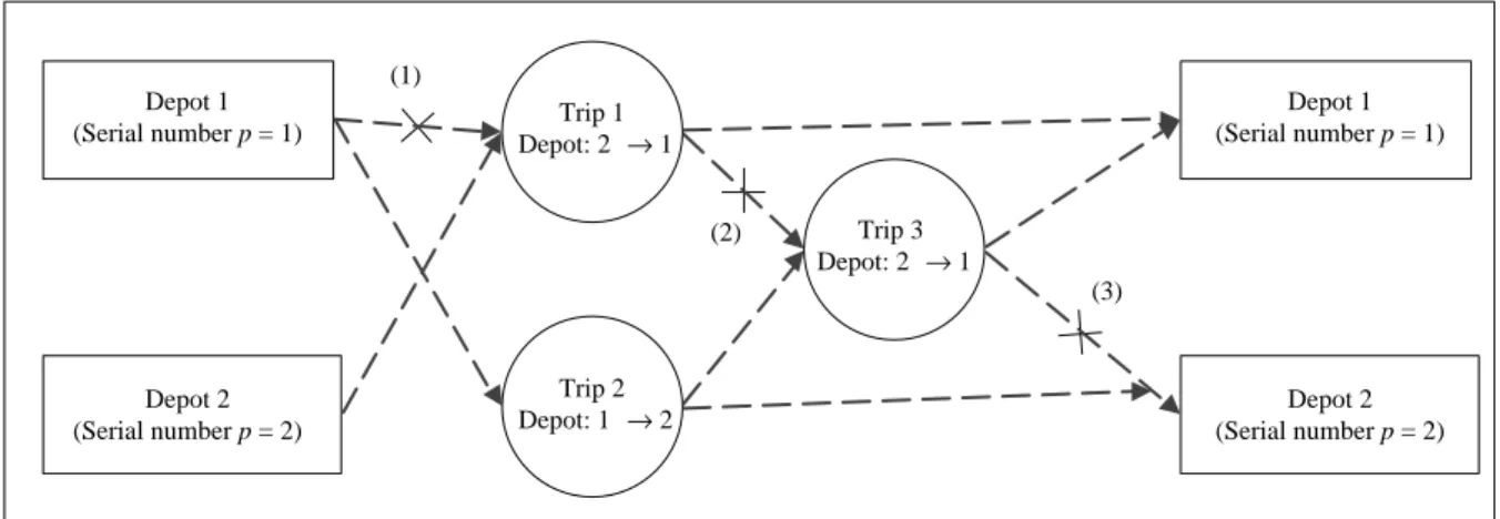
Equation (2) is a flow conservation constraint which makes sure the number of arcs leaving a trip is equal to the arcs entering the same trip. Eq. (3) is a constraint to ensure that each trip is served by one and only one vehicle. Eqs. (4), (5), and (6) can be regarded as Either-Or constraints which limit the chance of a deadhead trip occurring. Eq. (4) prohibits deadhead occurrence from depots to any trips when the serial number of a depot is not the same as departure termi-nal of a trip, as Fig. 2 shows. Based on this constraint, if p (number of depots) is not the same as sj (departure
terminal of trip j), then the variable xpn + p, j must be
equal to zero. This ensures that a deadhead trip from Depot 1 (Serial number p = 1) Depot 2 (Serial number p = 2) Trip 1 Depot: 2 → 1 Trip 2 Depot: 1 → 2 Trip 3 Depot: 2 → 1 (1) Depot 1 (Serial number p = 1) Depot 2 (Serial number p = 2) (2) (3)
(1) It makes sure that deadhead occurring from depot 1 to departure terminal of trip 1 will not happen when Eq. (4) exists in the model formulation.
(2) It makes sure that no deadhead occurrence between trip 1 and trip 3 when Eq. (6) exists in the model formulation.
(3) It makes sure that deadhead occurring from arrival terminal of trip 3 to depot 2 will nothappenwhen Eq. (5) exists in the model formulation.
Fig. 2 Example of explanation for Eqs. (4), (5), and (6)
a depot p to departure terminal of trip j will not hap-pen in any block. Eq. (5) is similar to Eq. (4), which prohibits a deadhead trip from any trips to depots when arrival terminal of that trip is not the same as the se-rial number of a depot, as Fig. 2 shows. In this constraint, if p is not the same as ei (arrival terminal of trip i),
then the variable xpi, n + p must be equal to zero. This
ensures that a deadhead trip from arrival terminal of trip i to a depot p will not happen in any block. Likewise, Eq. (6) ensures no deadhead occurrence between any two trips when arrival terminal of a trip is not the same as departure terminal of the other trip, as Fig. 2 shows. According to this constraint, if sj is not the same as ei,
then the variable xijp must be equal to zero. Eq. (7)
indicates all variables are binary. The solution for this MDVSP problem formulation finds a set of blocks to minimize the objective value so an ideal vehicle allo-cation plan with a minimal fleet size can be identified. 3. Deadhead Trips Adopting Strategies
Deadhead trips can be classified into two categories, the “depot deadhead trip” occurring be-tween depot and trip, and the “street deadhead trip” occurring between two trips. The deadhead trip is a common status in vehicle scheduling problems. The current study adopts four strategies representing dead-head trip tolerance of these two categories. Constraint Eqs (4), (5) and (6), defined below, decide the differ-ent strategies.
(1) All depot deadhead trips and street dead-head trips are allowed: Eqs. (4), (5) and (6) should be included in the model.
(2) Depot deadhead trips are allowed and street deadhead trips are not allowed: Eqs. (4) and (5) should be included in the model. (3) Depot deadhead trips are not allowed and
street deadhead trips are allowed: only Eq. (6) should be included in the model. (4) All depot deadhead trips and street
dead-head trips are not allowed: none of Eqs. (4), (5) or (6) should be included in the model. If the fourth strategy is adopted, the total num-ber of trips departing from each depot must be equal to the total number of trips returning to the same depot, i.e. Eq. (8) should be included in the model. Otherwise, the solution is not feasible.
xn + p, ip
Σ
i∈ N = xj, n + p pΣ
j∈ N ∀p ∈ P (8) III. A GREEDY HEURISTIC ALGORITHMFOR SOLVING THE MDVSP MODEL It is already known that the MDVSP is charac-terized as NP-hard when depot number exceeds two,
and the single depot problem can be solved in the polynomial time (Hadjar et al., 2006). The vehicle scheduling problem with single depot can be mod-eled as a minimum cost flow problem and solved with efficient algorithms to optimality (Gintner et al., 2005). This work develops a heuristics algorithm ap-plying the divide-and-conquer technique to solve the MDVSP model, according to the above-mentioned discussion.
1. Problem Solving Procedure
According to the graph theory concept, the pro-posed MDVSP formulation includes P networks, where P is the number of depots (i.e. there are P de-pots-as-nodes). There are N trips-as-nodes in each network, where N is the total number of trips. Besides, all networks correspond to P depots-as-nodes. Under the proposed heuristic algorithm, the MDVSP can be divided into several simplified sets of networks based on P depots. Each network corre-sponds to a single depot vehicle scheduling problem (SDVSP), while each problem takes into account all depots. Select a SDVSP associated with the chosen depot from the MDVSP formulation as a starting point, and ignore other models for a moment. Mathematically, the simplified SDVSP can be solved efficiently. Follow this with a search for feasible blocks in which depot deadhead trips are not allowed for the chosen depot. The variables for these fea-sible blocks are fixed in the following searches. This process narrows the search scope and increases search efficiency in the remaining SDVSP models. The problem solving procedure repeats until every depot is selected and the MDVSP solution is obtained by aggregating all feasible SDVSP solutions.
This heuristic can be regarded as a greedy algorithm, and the process of solving each SDVSP model considers all the interactions between the total num-ber of trips and all depots. A greedy algorithm can generally achieve a solution by making sequential choices, each of which simply looks at the best choice at the moment (Neapolitan and Naimipour, 2004). The traditional greedy rule performs following a defined criterion which satisfies some local optimal consider-ations at a time. According to the requirement of MDVSP, it is regarded as a reasonable rule for find-ing the maximum number of trips served by each de-pot in the proposed greedy heuristic algorithm. It is known that, although a greedy algorithm is no guar-antee of an optimal solution, one often leads to an ef-ficient solution fast (Neapolitan and Naimipour, 2004). This solving procedure can be defined as below: Step 1. Assign depot number in ascendant order fol-lowing the number of trips. And divide the given MDVSP formulation into a set of
SDVSP models. Step 2. Set p := 1.
Step 3. If p := |P|, go to Step 7, otherwise proceed to Step 4.
Step 4. Solve the SDVSP with an efficient algorithm while only considering depot p.
Step 5. Add every feasible block in which depot deadhead trips are not allowed into set S and fix the variables in these feasible blocks. Step 6. Define, p := p + 1, and proceed to Step 3. Step 7. Output set S as a final solution to the given
MDVSP.
2. Selection Rule for A Starting Point in the Greedy Heuristic Algorithm
Selecting a good starting point rule is generally an important step for a greedy algorithm. Each de-pot is first assigned a serial number continuously fol-lowing the number of trips in our solving procedure. This study adopts three different rules to precede problem computation: Following increasing order, decreasing order, and random order of depots in or-der to compare the results of selecting different rules. The selection rules are described as follows.
(a) Select depots following increasing serial number order: This heuristic algorithm first divides the given MDVSP into a serial of SDVSP’s following an increasing depot number order. The solution procedure is in-troduced in section III.
(b) Select depot following decreasing serial number order: The steps of this heuristic algorithm are similar to (a), except for fol-lowing the decreasing order of depot serial number. The solution procedure is the same as the one mentioned in section III except steps 2, 3 and 6 are replaced by:
Step 2. Set p := |P|, and ignore the other de-pots for a moment.
Step 3. If p := 1 go to Step 7, otherwise pro-ceed to Step 4.
Step 6. Define p := p – 1, and returns to Step 3.
(c) Select depot serial number arbitrarily: The steps of this heuristic algorithm are also similar to both heuristics mentioned above, except instead of following the increasing or decreasing order of depot serial numbers, it selects the depot serial number arbitrarily. The solution procedure is also similar to the one mentioned in section III except that Step 2, 3 and 6 are replaced by the following: Step 2. Set U = P. Select an initial depot
arbitrarily pi∈ U, and U = U – pi.
Step 3. If U = ∅, go to Step 7, otherwise
proceed to Step 4.
Step 6. Select another depot arbitrarily pj∈
U, and define U = U – pj, then return
to Step 3.
IV. COMPUTATIONAL TESTS 1. Results of A Case Study
The adopted greedy heuristic solving procedures solve a real case to demonstrate the efficiency and effectiveness of the proposed formulation and the heuristic algorithm. A MDVSP model is set up to replicate the situation occurring in the Kinmen Bus Administration (KBA). The theoretical optimal so-lution and existing arrangement are used to compare with solutions obtained by the proposed problem solv-ing algorithms. The computations are executed on a personal computer with a Pentium-IV CPU 3.2GHz and 3.25GB main memory. All models in the numeri-cal experiments are solved with ILOG CPLEX 7.0.
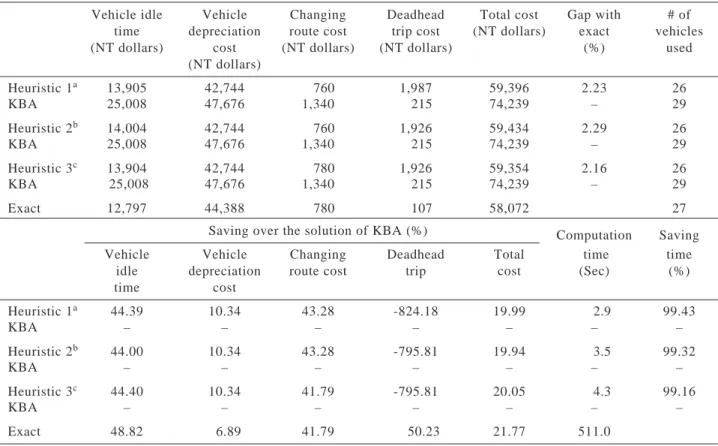
The KBA case includes three depots, A, B, C, currently serving six routes (A-A, A-B, A-C, B-B, B-C, C-C). Twenty-nine vehicles are operated daily, offering a total of 395 trips. The three starting point selection rules have all show possible computation result differences. The parameters’ values provided by the manager in the KBA case are set as follows: α = 3.33(NT dollar/min), β = 1,644(NT dollar/per ve-hicle per day), λ = 10 (NT dollar/per round), and ω = 4.67(NT dollar/min).
The experiments adopt only the strategy of all depot deadhead trips and street deadhead trips are allowed, for computation convenience. Table 1 shows the computation results. Compared to the existing arrangement represented as KBA, the solutions ob-tained by the three different starting point selection rules reduce the total cost by 19.99%, 19.94%, and 20.05% respectively. Similarly, compared to KBA, the theoretical optimal solution reduces the total cost by 21.77%, showing that the solutions obtained by the proposed heuristic algorithms are close to the optimal solution. Cost saving mainly comes from improving vehicle idle time and preventing unnecessary route changing. Improved vehicle idle time percentages are from 44.00% to 44.40%, the theoretical optimal so-lution improves 48.82%. Improved percentages on cost of changing route are from 41.79% to 43.28%, the theoretical optimal solution improves 41.79%. Three vehicles are saved by all three selection rules apply-ing in the heuristic algorithm and the percentage of vehicle capital cost saving are all 10.34%. The sav-ings of deadhead trips cost in the three results ob-tained by the heuristic algorithm are all worse than KBA and the theoretical optimal solution. This re-sult shows that applying the heuristic algorithm is not
necessarily a guarantee of saving improvement in all cost items. Compared to the theoretical optimal solution, the total cost reduction obtained by the heuristic al-gorithm using the three different starting point selec-tion rules ranges from 2.16% to 2.29%, close enough in this case. The computation times of the heuristic algorithm by three different starting point selection rules are all significantly less than that for finding the theoretical optimal solution. The time saving rates are 99.43%, 99.32% and 98.16% by three different selection rules respectively. This result indicates that the heuristic approach solves the MDVSP much more efficiently, a very important result in practical applica-tion.
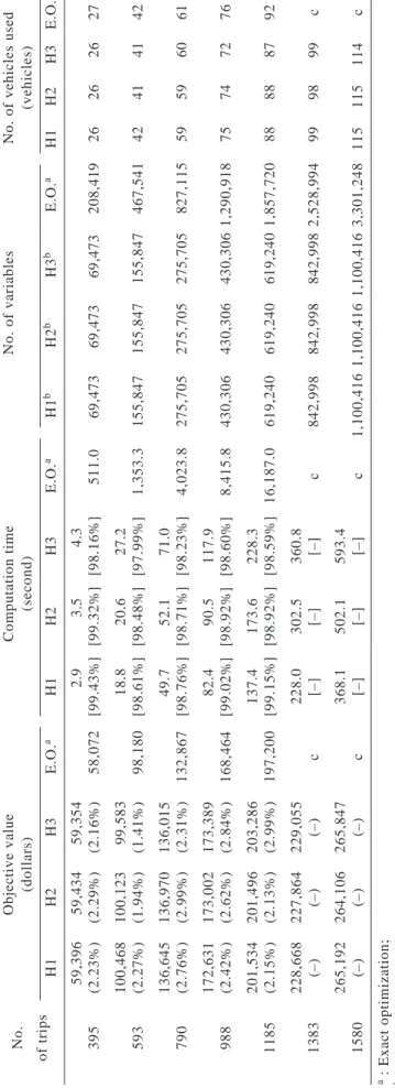
This research modifies the KBA case by adding the number of trips arbitrarily to evaluate the perfor-mance of the greedy algorithm applied to a larger scale problem such as a global airline or maritime operation. Testing is conducted for cases composing 593, 790, 988, 1,185, 1,383, and 1,580 trips. Table 2 summa-rizes computation results. Findings show that the number of variables in the problem increases significantly fol-lowing the increasing problem scale (i.e numbers of trips). The result shows that under the same computer
processing capability, the optimal solution cannot be found if the number of trips exceeds 1,383. The re-sult also shows that compared to objective values in solutions obtained by the heuristic algorithm compared to theoretical optimal solutions, differences remain within the range of 1.41% to 2.99%. Computation times on the other hand, save more than 97.99%.
2. Sensitivity Analysis of the MDVSP Parameter Values
Sensitivity analysis shows the difference in re-sults by changing MDVSP parameter values. The two important parameters adopted in the proposed MDVSP model are vehicle depreciation cost and cost of deadhead trips per minute because the necessary fleet size in the KBA case is a crucial concern for decision makers and the savings of deadhead trips cost in the three results obtained by the heuristic algorithm are all worse than KBA and the theoretical optimal solution. For testing purposes, ten different scenarios for each parameter value scenario (vehicle deprecia-tion cost, deadhead trip cost) are increased 10% arbi-trarily every time (seen Table 3).
Table 1 Test results for the KBA problem
Note: The exchange rate was NT $1 = US $0.03051 Vehicle idle Vehicle Changing Deadhead Total cost Gap with # of
time depreciation route cost trip cost (NT dollars) exact vehicles
(NT dollars) cost (NT dollars) (NT dollars) (%) used
(NT dollars) Heuristic 1a 13,905 42,744 760 1,987 59,396 2.23 26 KBA 25,008 47,676 1,340 215 74,239 – 29 Heuristic 2b 14,004 42,744 760 1,926 59,434 2.29 26 KBA 25,008 47,676 1,340 215 74,239 – 29 Heuristic 3c 13,904 42,744 780 1,926 59,354 2.16 26 KBA 25,008 47,676 1,340 215 74,239 – 29 Exact 12,797 44,388 780 107 58,072 27
Saving over the solution of KBA (%) Computation Saving
Vehicle Vehicle Changing Deadhead Total time time
idle depreciation route cost trip cost (Sec) (%)
time cost Heuristic 1a 44.39 10.34 43.28 -824.18 19.99 2.9 99.43 KBA – – – – – – – Heuristic 2b 44.00 10.34 43.28 -795.81 19.94 3.5 99.32 KBA – – – – – – – Heuristic 3c 44.40 10.34 41.79 -795.81 20.05 4.3 99.16 KBA – – – – – – – Exact 48.82 6.89 41.79 50.23 21.77 511.0
a: Using the selection rule with increasing order of depot serial number b: Using the selection rule with decreasing order of depot serial number c: Using the selection rule with depot serial number at random
Table 2 Test results for six scenarios
Objective value
Computation time
No. of variables
No. of vehicles used
No. (dollars) (second) (vehicles) of trips H1 H2 H3 E.O. a H1 H2 H3 E.O. a H1 b H2 b H3 b E.O. a H1 H2 H3 E.O. a 59,396 59,434 59,354 2 .9 3 .5 4 .3 395 (2.23%) (2.29%) (2.16%) 58,072 [99.43%] [99.32%] [98.16%] 511.0 69,473 69,473 69,473 208,419 2 6 2 6 2 6 2 7 100,468 100,123 99,583 18.8 20.6 27.2 593 (2.27%) (1.94%) (1.41%) 98,180 [98.61%] [98.48%] [97.99%] 1,353.3 155,847 155,847 155,847 467,541 4 2 4 1 4 1 42 136,645 136,970 136,015 49.7 52.1 71.0 790 (2.76%) (2.99%) (2.31%) 132,867 [98.76%] [98.71%] [98.23%] 4,023.8 275,705 275,705 275,705 827,115 5 9 5 9 6 0 61 172,631 173,002 173,389 82.4 90.5 117.9 988 (2.42%) (2.62%) (2.84%) 168,464 [99.02%] [98.92%] [98.60%] 8,415.8 430,306 430,306 430,306 1,290,918 7 5 7 4 7 2 76 201,534 201,496 203,286 137.4 173.6 228.3 1185 (2.15%) (2.13%) (2.99%) 197,200 [99.15%] [98.92%] [98.59%] 16,187.0 619,240 619,240 619,240 1,857,720 8 8 8 8 8 7 92 228,668 227,864 229,055 228.0 302.5 360.8 1383 (–) (–) (–) c [–] [–] [–] c 842,998 842,998 842,998 2,528,994 9 9 9 8 9 9 c 265,192 264,106 265,847 368.1 502.1 593.4 1580 (–) (–) (–) c [–] [–] [–] c 1,100,416 1,100,416 1,100,416 3,301,248 115 115 114 c
a : Exact optimization; b : This value is the most variables in three submodels; c :The 1,383 and 1,580 trips can not be solved by the exact optimization on the test machine; ( ) : The percentage in parentheses is the gap with optimal solution; [ ] : The percentage in braces is the time-saving rate.
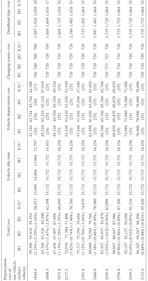
Table 3 Sensitivity analysis of depreciation cost for the KBA problem
The exchange rate was NT $1 = US $0.03051
Depreciation cost of
Total cost
Vehicle idle time
Vehicle depreciation cost
Changing routes cost
Deadhead trips cost
one vehicle (dollars/
H1 H2 H3 E.O. a H1 H2 H3 E.O. a H1 H2 H3 E.O. a H1 H2 H3 E.O. a H1 H2 H3 E.O. a vehicle) 59,396 59,434 59,354 42,744 42,744 42,744 44,388 1644.0 (2.23%) (2.29%) (2.16%) 58,072 13,905 14,004 13,904 12,797 [26] [26] [26] [27] 760 760 780 780 1,987 1,926 1,926 107 63,326 63,326 63,588 45,210 45,210 45,210 47,018 1808.4 (1.47%) (1.47%) (1.87%) 62,398 15,732 15,732 15,732 14,453 [26] [25] [25] [25] 720 720 720 750 1,664 1,664 1,926 177 67,436 67,497 67,698 49,320 49,320 49,320 49,320 1972.8 (1.17%) (1.25%) (1.55%) 66,650 15,732 15,732 15,732 16,256 [25] [25] [25] [25] 720 720 720 720 1,664 1,725 1,926 354 2137.2 72,070 71,284 71,808 53,430 53,430 53,430 53,430 (1.82%) (0.74%) (1.46%) 70,760 15,732 15,733 15,733 16,256 [25] [25] [25] [25] 720 720 720 720 2,188 1,402 1,926 354 75,717 75,394 75,656 57,540 57,540 57,540 57,540 2301.6 (1.12%) (0.70%) (1.04%) 74,870 15,732 15,733 15,733 16,256 [25] [25] [25] [25] 720 720 720 720 1,725 1,402 1,664 354 80,089 79,504 79,766 61,650 61,650 61,650 61,650 2466.0 (1.38%) (0.66%) (0.99%) 78,980 15,732 15,732 15,732 16,256 [25] [25] [25] [25] 720 720 720 720 1,987 1,402 1,664 354 83,937 83,937 83,876 65,760 65,760 65,760 65,760 2630.4 (1.01%) (1.01%) (0.94%) 83,090 15,732 15,732 15,732 16,256 [25] [25] [25] [25] 720 717 723 720 1,725 1,725 1,664 354 88,047 88,047 87,986 69,870 69,870 69,870 69,870 2794.8 (0.96%) (0.96%) (0.89%) 87,200 15,732 15,732 15,732 16,256 [25] [25] [25] [25] 720 720 720 720 1,725 1,725 1,664 354 92,157 92,157 92,096 73,980 73,980 73,980 73,980 2959.2 (0.92%) (0.92%) (0.85%) 91,310 15,732 15,732 15,732 16,256 [25] [25] [25] [25] 720 720 720 720 1,725 1,725 1,664 354 96,267 96,267 96,206 78,090 78,090 78,090 78,090 3123.6 (0.88%) (0.88%) (0.82%) 95,420 15,732 15,733 15,733 16,256 [25] [25] [25] [25] 720 720 720 720 1,725 1,725 1,664 354
a : Exact Optimization; ( ) : The percentage in parentheses is the gap with optimal solution; [ ] : The value in braces is the number of vehicles used.
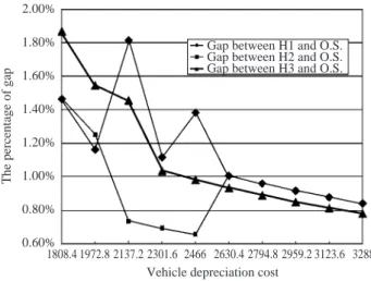
The first sensitivity analysis shows the difference in resulting from changing vehicle depreciation cost. Table 3 shows that total cost increases if vehicle de-preciation cost increases. But it is quite obvious that the other three cost items, such as vehicle idle time, changing routes and deadhead trips, all remain the same no matter which starting point selection rule is adopted while vehicle depreciation cost exceeds 2,630.4. The total cost increases steadily as vehicle depreciation cost increases, as shown. Results show that vehicle depre-ciation cost is insensitive to the other three cost items and total cost while the value is larger than 2,630.4. When vehicle depreciation cost reaches 1972.8, the number of required vehicles remains twenty-five, which seems to be the minimum number needed in the KBA case. Results show that the difference between the results of total cost obtained by the heuristic algorithm and the theoretical optimal solution reduce as vehicle depreciation cost increases. Fig. 3 shows the percent-age of gap between the heuristic algorithm using the three different starting point selection rules and the theoretical optimal solutions versus vehicle deprecia-tion cost for the KBA.
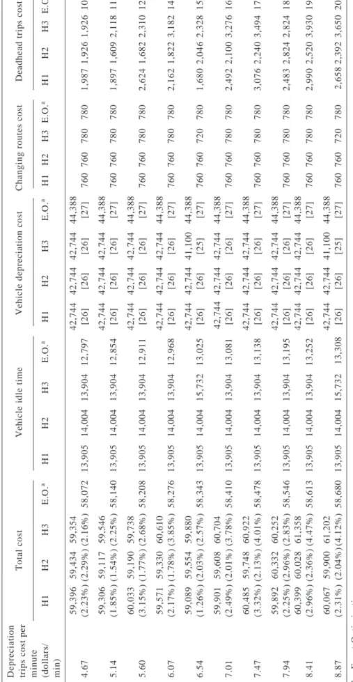
The second sensitivity analysis shows the dif-ference in results from changing deadhead trip cost. Table 4 again shows that total cost increases if dead-head trip cost increases. Results in the ten scenarios show that vehicle idle time costs remain nearly the same for each selection rule, but compared to the theo-retical optimal solution, the vehicle idle time costs increase as deadhead trip costs increase. Deadhead trip cost on the other hand, seems to have no effect on vehicle depreciation costs and changing routes cost because vehicle depreciation cost and changing routes cost remain nearly the same. Results show that dead-head trip cost has little impact on solutions obtained by the heuristic algorithm, but has most effect on the
2.00% 1.80% 1.60% 1.40% 1.20% 1.00% 0.80% 0.60% 1808.4 1972.8 2137.2 2301.6 2466 2630.4 Vehicle depreciation cost
2794.8 2959.2 3123.6 3288
The percentage of gap
Gap between H1 and O.S. Gap between H2 and O.S. Gap between H3 and O.S.
Fig. 3 The percentage of gap between the heuristic algorithms
and the theoretical optimal solutions (o.s.) vs. vehicle de-preciation cost
theoretical optimal solution. A large gap in dead-head trip cost between the heuristic algorithm using the three different starting point selection rules and the theoretical optimal solution exists, as shown. This gap indicates that the difference between total cost obtained by the heuristic algorithm and the theoreti-cal optimal solution is mostly reflected in deadhead trip cost. Results also show that the differences be-tween the results of total cost obtained by the heuris-tic algorithm and the theoreheuris-tical optimal solution tend to increase as deadhead trip cost increases. Fig. 4 shows the percentage of gap between the heuristic algorithm using the three different starting point se-lection rules and the theoretical optimal solutions ver-sus deadhead trip cost for the KBA.
V. CONCLUSIONS
This paper presents a new model formulation for the MDVSP for public transit services. This study also proposes a greedy heuristic algorithm based on divide-and-conquer technique to solve the MDVSP. Performances of the proposed model and the heuris-tic algorithm have been shown to be very efficient based on real case data provided by the KBA. Solu-tion results are also reasonably close to the theoreti-cal optimal solution. Computer running time can be reduced more than 98.16% compared to the theoreti-cal optimal solution. The problem-solving algorithm also provides better capability to deal with lager scale problems (representing more depots and trips). Sen-sitivity analyses also show that the lower bound of vehicle depreciation cost leading to the minimum number of required vehicles seems to exist in in-stances of MDVSP. The analyses also show that the greater the vehicle depreciation cost, the closer the solutions obtained by the heuristic algorithm are to the theoretical optimal solution, but the greater the deadhead trip cost, the further the solutions obtained by the heuristic algorithm are from the theoretical optimal solution conversely. Excellent computation efficiency, good larger scale problem solving capability, and good quality solution, all suggest that the findings in this study probably shorten the dis-tance between a theoretical study and practical ap-plication in dealing with real world problems.
The transportation industry, while considering the vehicle scheduling problem, needs to combine the arrangement needs of both vehicles and crew. Crew assignment is not discussed in this study at this time. Exploring this issue in the future would be interesting. Fortunately, compared to traditional problem definitions, the proposed model formulation and problem-solv-ing algorithm provide excellent computation capability. The model also provides a better chance to solve this type of problem. Techniques for solving the MDVSP
Table 4 Sensitivity analysis of deadhead trips cost for the KBA problem
The exchange rate was NT $1 = US $0.03051
Depreciation trips cost per
Total cost
Vehicle idle time
Vehicle depreciation cost
Changing routes cost
Deadhead trips cost
minute (dollars/ H1 H2 H3 E.O. a H1 H2 H3 E.O. a H1 H2 H3 E.O. a H1 H2 H3 E.O. a H1 H2 H3 E.O. a min) 59,396 59,434 59,354 42,744 42,744 42,744 44,388 4.67 (2.23%) (2.29%) (2.16%) 58,072 13,905 14,004 13,904 12,797 [26] [26] [26] [27] 760 760 780 780 1,987 1,926 1,926 107 59,306 59,117 59,546 42,744 42,744 42,744 44,388 5.14 (1.85%) (1.54%) (2.25%) 58,140 13,905 14,004 13,904 12,854 [26] [26] [26] [27] 760 760 780 780 1,897 1,609 2,118 118 60,033 59,190 59,738 42,744 42,744 42,744 44,388 5.60 (3.15%) (1.77%) (2.68%) 58,208 13,905 14,004 13,904 12,911 [26] [26] [26] [27] 760 760 780 780 2,624 1,682 2,310 129 59,571 59,330 60,610 42,744 42,744 42,744 44,388 6.07 (2.17%) (1.78%) (3.85%) 58,276 13,905 14,004 13,904 12,968 [26] [26] [26] [27] 760 760 780 780 2,162 1,822 3,182 140 59,089 59,554 59,880 42,744 42,744 41,100 44,388 6.54 (1.26%) (2.03%) (2.57%) 58,343 13,905 14,004 15,732 13,025 [26] [26] [25] [27] 760 760 720 780 1,680 2,046 2,328 150 59,901 59,608 60,704 42,744 42,744 42,744 44,388 7.01 (2.49%) (2.01%) (3.78%) 58,410 13,905 14,004 13,904 13,081 [26] [26] [26] [27] 760 760 780 780 2,492 2,100 3,276 161 60,485 59,748 60,922 42,744 42,744 42,744 44,388 7.47 (3.32%) (2.13%) (4.01%) 58,478 13,905 14,004 13,904 13,138 [26] [26] [26] [27] 760 760 780 780 3,076 2,240 3,494 172 59,892 60,332 60,252 42,744 42,744 42,744 44,388 7.94 (2.25%) (2.96%) (2.83%) 58,546 13,905 14,004 13,904 13,195 [26] [26] [26] [27] 760 760 780 780 2,483 2,824 2,824 183 60,399 60,028 61,358 42,744 42,744 42,744 44,388 8.41 (2.96%) (2.36%) (4.47%) 58,613 13,905 14,004 13,904 13,252 [26] [26] [26] [27] 760 760 780 780 2,990 2,520 3,930 193 60,067 59,900 61,202 42,744 42,744 41,100 44,388 8.87 (2.31%) (2.04%) (4.12%) 58,680 13,905 14,004 15,732 13,308 [26] [26] [25] [27] 760 760 720 780 2,658 2,392 3,650 204
a : Exact Optimization; ( ) : The percentage in parentheses is the gap with optimal solution; [ ] : The value in braces is the number of vehicles used.
are still looking for a method that improves the gap of deadhead trip cost between the heuristic algorithm and the theoretical optimal solution in order to en-hance solution quality. Finally, we hope that the findings in this study can be applied to develop a decision sup-porting system to help solve real-world vehicle sched-uling problems, not just for the local public transit industry, but also for the global transportation indus-try (including airline and maritime industries).
ACKNOWLEDGEMENTS
We thank Kinmen Bus Administration for pro-viding the test data and their valuable opinions.
NOMENCLATURE A arcs in graph
cij arc cost
ei arrival depot
G graph representation
i, j specific trip in known trip set I feasible set of pairs of trips li length of service time, or duration
n number of trips N trip set
Oci cost of serving the trip
p specific depot in known depot set P depot set
si departure depot
U temporary set of depot set V vertexes in graph
xijp flow for type p through arc (i, j) ∈ Ap
Greek Symbols
α cost for vehicle idle time (dollars/min)
β cost for half of the depreciation per vehicle (dollars/vehicle)
γi specific route number
λ cost/penalty for every time changing route in a block (dollars/per change)
τi departure time
ξij travel time from the end depot of trip i to the
start depot of trip j
ω cost of deadhead trips per minute (dollars/min) REFERENCE
Baita, F., Pesenti, R., Ukovich, W., and Favaretto, D., 2000, “A Comparison of Different Solution Approaches to the Vehicle Scheduling Problem in a Practical Case,” Computers & Operations Re-search, Vol. 27, No. 13, pp. 1249-1269.
Ball, M. O., Magnanti, T. L., Monma, C. L., and Nemhauser, G. L., 1995, “Ch2. Time Constrained Routing and Scheduling,” Handbooks in Opera-tion Research and Management Sciences- Net-work Routing, Vol. 8, Elsevier Science B.V., Amsterdam, the Netherlands.
Beasley, J. E., and Cao, B., 1996, “A Tree Search Algorithm for the Crew Scheduling Problem,” European Journal of Operational Research, Vol. 94, No. 3, pp. 517-526.
Bertossi, A. A., Carraresi, P., and Gallo, G., 1987, “On Some Matching Problems Arising in Vehicle Scheduling Models,” Networks, Vol. 17, No. 3, pp. 271-281.
Bodin, L., Golden B., Assad A., and Gall, M., 1983, “Routing and Scheduling of Vehicles and Crews – the State of the Art,” Computers & Operations Research, Vol. 10, No. 1, pp. 63-211.
Bodin, L., and Golden, B., 1981, “Classification in Vehicle Routing and Scheduling,” Networks, Vol. 11, No. 2, pp.97-108.
Carraresi, P., and Gallo, G., 1983, “Network Models for Vehicle and Crew Scheduling,” European Journal of Operational Research, Vol. 16, No. 3, pp. 139-151.
Carpaneto, G., Dell, Amico, M., Fischetti, M., and Toth, P., 1989, “A Branch and Bound Algorithm for the Multiple Vehicle Scheduling Problem,” Networks, Vol. 19, No. 5, pp. 531-548.
Cordeau, J., Laporte, G., and Mercier, A., 2001, “A Unified Tabu Search Heuristic for Vehicle Rout-ing Problems with Time Windows,” Journal of the Operational Research Society, Vol. 52, No. 8, pp. 928-936.
Daduna, J., and Paixão, J., 1995, “Vehicle Schedul-ing for Public Mass Transit- an Overview,” Pro-ceedings of the Sixth International Workshop on Computer-Aided Scheduling of Public Transport, Lisbon, Portugal, pp. 76-90.
Fig. 4 The percentage of gap between the heuristic algorithms
and the theoretial optimal solutions (o.s.) vs. deadhead trip cost 4.50% 4.00% 3.50% 3.00% 2.50% 2.00% 1.50% 1.00% 5.14 5.6 6.07 6.54 7.01 7.47
Deadhead trip cost
7.94 8.41 8.87 9.34
The percentage of gap
Gap between H1 and O.S. Gap between H2 and O.S. Gap between H3 and O.S.
Desaulniers, G., Desrosiers, J., Dumas, Y., Marc, S., Rioux, B., Solomon, M. M., and Soumis, F., 1997, “Crew Pairing at Air France,” European Journal of Operational Research, Vol. 97, No. 2, pp. 245-259.
Forbes, M. A., Hotts, J. N., and Watts, A. M., 1994, “An Exact Algorithm for Multiple Depot Vehicle Scheduling,” European Journal of Operational Research, Vol. 72, No. 1, pp. 115-124.
Ford, L. R., and Fulkerson, D. R., 1962, Flows in Networks, Princeton University Press, N. J., USA. Freling, R., 1997, “Models and Techniques for Inte-grating Vehicle and Crew Scheduling,” Ph. D. Thesis, Tinbergen Institute, Erasmus University, Rotterdam, the Netherlands.
Gintner, V., Kliewer, N., and Suhl, L., 2005, “Solv-ing Large Multiple-depot Multiple-vehicle-type Bus Scheduling Problems in Practice,” OR Spectrum, Vol. 27, No.4, pp. 507-523.
Hadjar, A., Marcotte, O., and Soumis, F., 2006, “A Branch-and-Cut Algorithm for the Multiple De-pot Vehicle Scheduling Problem,” Operations Research, Vol. 54, No. 1, pp. 130-149.
Haghani, A., Banihashemi, M., and Chiang, K. H., 2003, “A Comparative Analysis of Bus Transit Vehicle Scheduling Models,” Transportation Research Part B, Vol. 37, No. 4, pp. 301-322. Haghani, A., and Banihashemi, M., 2002, “Heuristic
Approached for Solving Large-scale Bus Transit Vehicle Scheduling Problem with Route Time Constraints,” Transportation Research Part A, Vol. 36, No. 4, pp. 309-333.
ILOG, 2000, Cplex v7.0 User’s Manual, Gentilly, France.
Kliewer, N., Mellouli, T., and Suhl, L., 2006, “A Time-space Network Based Exact Optimization Model for Multi-depot Bus Scheduling,” Euro-pean Journal of Operational Research, Vol. 175, No. 3, pp. 1616-1627.
Kolott, A., and Löbel, A., 1996, “Lagrangean Relax-ations and Subgradient Methods for Multiple-De-pot Vehicle Scheduling Problems,” ZIB-Report, Konrad-Zuse-Zentrum für Informationstchnik, Berlin, Germany, pp. 96-22.
Lamatsch, A., 1992, “An Approach to Vehicle Sched-uling with Depot Capacity Constraints,” Com-puter-Aided Transit Scheduling, Lecture Notes in Economics and Mathematical Systems 386, Springer- Berlag, Berlin, Germany, pp. 181-195. Lavoie, S., Minoux, M., and Odier, E., 1988, “A New Approach for Crew Pairing Problems by Column Generation with an Application to Air Transporta-tion,” European Journal of Operational Research, Vol. 35, No. 1, pp. 45-58.
Löbel, A., 1997, “Solving Large-Scale Multiple-Ddepot Scheduling Problems,” Proceedings of the 7th International Conference on Computer-aided Scheduling of Public Transit, Cambridge, MA, USA, pp. 193-220.
Mesquita, M., and Paixão, J., 1990, “Multiple Depot Vehicle Scheduling Problem: A New Heuristic Based on Quasi-assignment Algorithm,” Proceed-ings of the 5th International Conference on Com-puter-aided Scheduling of Public Transit, Montreal, Canada.
Neapolitan, R., and Naimipour, K., 2004, Founda-tions of Algorithms-Using C++ Pseudocode, 3rd ed., Jones and Bartlett Publishers, Massachusetts, USA.
Orloff, C. S., 1976, “Route Constrained Fleet Schedul-ing,” Transportation science, Vol. 10, No. 2, pp. 149-168.
Paixao, J., and Branco, I. M., 1987, “A Quasi-Assign-ment Algorithm for Bus Scheduling,” Networks, Vol. 17, No. 3, pp. 249-270.
Pepin, A., Desaulniers, G., Hertz, A., and Huisman, D., 2006, “Comparison of Heuristic Approaches for the Multiple Depot Vehicle Scheduling Problem,” Odysseus 2006, Altea, Spain (23-26 mai), pp. 1-27.
Ribeiro, C., and Soumis, F., 1994, “A Column Gen-eration Approach to the Multiple Depot Vehicle Scheduling Problem,” Operations Research, Vol. 42, No. 1, pp. 41-52.
Su, J. M. and Yu, W. S., 2006, “Single-Depot Bus Drivers and Vehicles Scheduling Problem,” Transportation Planning Journal, Quarterly, Vol. 35, No. 2, pp.131-157.
Wang, J. Y., and Lin, C. K., 2006, “A Generic Vehicle Scheduling Model for Inter-city Bus Car-riers under Fixed-timetable,” Transportation Planning Journal, Quarterly, Vol. 35, No. 1, pp. 107-130.
Wang, J. Y., and Lin, C. K., 2003, “Deployment Promotion Project of the Core Modules of Fleet Management System for Public Transportation,” Report No. 93-44-4281 Institute of Transportation, Ministry of Transportation And Communications, Taiwan, ROC.
Yan., S., and Tu, Y. P., 2002, “A Network Model for Airline Cabin Crew Scheduling,” European Jour-nal of OperatioJour-nal Research, Vol. 140, No. 3, pp. 531-540.
Manuscript Received: Feb. 20, 2008 Revision Received: Jan. 28, 2009 and Accepted: Feb. 28, 2009