應用於數位電視之H.264/AVC背景適應性二元算術解碼器

國立交通大學

電子工程學系 電子研究所碩士班

碩 士 論 文

應用於數位電視之 H.264/AVC 背景適應性二元算術解

碼器

Context Adaptive Binary Arithmetic Decoder of

H.264/AVC for Digital TV Application

學生 ： 黃 毅 宏

指導教授 ：李鎮宜 教授

應用於數位電視之 H.264/AVC 背景適應性二元算術解

碼器

Context Adaptive Binary Arithmetic Decoder of

H.264/AVC for Digital TV Application

研 究 生：黃毅宏 Student：Yi-Hong Huang

指導教授：李鎮宜 Advisor：Chen-Yi Lee

國 立 交 通 大 學

電子工程學系 電子研究所 碩士班

碩 士 論 文

Submitted to Department of Electronics Engineering & Institute of Electronics College of Electrical and Computer Engineering

National Chiao Tung University in Partial Fulfillment of the Requirements

for the Degree of Master of Science

in

Electronics Engineering July 2006

Hsinchu, Taiwan, Republic of China

應用於數位電視之 H.264/AVC 適應性算術解碼器

學生：黃毅宏 指導教授：李鎮宜 教授

國立交通大學

電子工程學系 電子研究所碩士班

摘要

Context Adaptive Binary Arithmetic Decoder of

H.264/AVC for Digital TV Application

Student：Yig-Hong Huang Advisor：Dr. Chen-Yi Lee

Department of Electronics Engineering

Institute of Electronics

National Chiao Tung University

ABSTRACT

In this thesis, we propose a high-throughput RAM-based Context Adaptive Binary Arithmetic Decoder (CABAD). Our proposal is realized by one 399x7 bits two-port SRAM for the context model and one 120x208 bits single-port SRAM for row-storage of the syntax element. We will offer three methods to improve the throughput of CABAD in order to overcome the data dependency of the sub-division intervals. Our proposed architecture can achieve 244,800 macroblocks (MB) per second in average for level 4.0. Therefore, it can play 1080HD video at 30 fps. Based on 0.13µm UMC CMOS Process, our CABAD design needs 163,573 gates with SRAM and operates at 200MHz.

誌 謝

Contents

Chapter 1 Introduction...

1.1 Motivation...1

1.2 Organization of thesis ...2

Chapter 2 Algorithm of CABAD for H.264/AVC...

2.1 Overview of CABAD decoding flow...4

2.2 Algorithm of arithmetic code...7

2.2.1 Basic binary arithmetic encoding algorithm ...7

2.2.2 Binary arithmetic decoding algorithm...9

2.2.2.1 Basic binary arithmetic decoding algorithm ...9

2.2.2.2 Advanced binary arithmetic decoding algorithm for H.264/AVC...11

2.3 Binarization decoding flow...15

2.3.1 Unary decoding flow ...15

2.3.2 Truncated unary decoding flow ...16

2.3.3 Fixed-length decoding flow ...17

2.3.4 Unary/k-th order Exp-Golomb decoding flow ...18

2.3.5 Special decoding flow...19

2.4 Context model organization ...20

2.5 Syntax elements for the neighbor blocks ...25

Chapter 3 Binary Arithmetic Decoder Engine...

3.1 Overview for CABAD...30

3.2 1st Decoding Flow - Architecture of the Arithmetic Decoders...33

3.2.1 Normal decoding flow...33

3.2.2 Bypass decoding flow...41

3.2.3 Terminal decoding flow...47

3.3 2nd Decoding Flow-Architecture of the Binarization Engine...48

3.4 Summary...53

Chapter 4 Memory System ...

4.1 Initialization of the context model...54

4.2 Context model SRAM...56

4.3 Row-storage memory system of the neighbor information...58

4.3.1 RS memory in MB level...58

4.3.2 RS memory in sub-MB level...60

4.4 Summary...65

Chapter 5 Simulation and Implementation Result for Digital TV

Application...

5.1 Simulation result...66

5.2 Chip implementation...78

5.3 Summary...82

Chapter 6 Conclusion and Future work ...

List of Figures

Figure 1 Block diagram of H.264/AVC for baseline profile ...4

Figure 2 Block diagram of H.264/AVC for main profile ...4

Figure 3 Bit-stream structure of H.264/AVC...5

Figure 4 CABAC encoder block diagram...6

Figure 5 CABAD block diagram ...7

Figure 6(a) Definition of MPS and LPS ...8

Figure 6(b) Sub-divided interval of MPS...8

Figure 6(c) Sub-divided interval of LPS ...8

Figure 7(a) Result of MPS subdivision...10

Figure 7(b) Result of LPS subdivision ...10

Figure 8 Flowchart of the normal decoding flow ...12

Figure 9 Flowchart of renormalization ...13

Figure 10 Flowchart of the bypass decoding flow...14

Figure 11 Flowchart of the terminal decoding flow ...14

Figure 12 Illustration of the neighbor location in macroblock level ...26

Figure 13 Illustration of the neighbor location for sub-macroblock level ...27

Figure 14 System architecture of CABAD...30

Figure 16 Percentage of the AD usage...33

Figure 17 Pipeline schedule of the normal decoding flow ...34

Figure 18 Hardware architecture of AD ...35

Figure 19 Example of the second case...36

Figure 20 Example of the third case...37

Figure 21 Timing diagram of the pipeline comparison ...40

Figure 22 Percentage of the number of the concatenate bypass decoding under executing 100 CIF frames of six sequences ...42,43,44 Figure 23 (a) Bypass decoding unit and (b) Organization of the multi-symbol bypass decoding...45

Figure 24 Simple logic function for “skip renormalization” control signal ...47

Figure 25 Finite state machine of the binarization engine ...48

Figure 26 Zig-Zag scan ...49

Figure 27 Hadamard transform for Luma DC ...50

Figure 28 Hadamard transform for Luma AC ...50

Figure 29 Hadamard transform for Luma ...51

Figure 30 Hadamard transform for Chroma DC ...51

Figure 31 Hadamard transform for Chroma AC...52

Figure 32 Zero-skip architecture ...52

Figure 33 Implementation of the context model initialization...55

Figure 34 Timing diagram of the context model initialization ...56

Figure 36 Implementation of the address generator of the context model SRAM ...57

Figure 37 Required SRAM depths of 7 frame types...59

Figure 38 Row-Storage SRAM relates to the decoded macroblocks...59

Figure 39 Timing schedule of RS SRAM ...60

Figure 40 Row-Storage SRAM relates to the decoded sub-macroblocks...61

Figure 41 Row-Storage SRAM relates to the decoded sub-macroblocks...62

Figure 42 Macroblock and sub-macroblock partition...63

Figure 43 SE value mapping for different block size...64

Figure 44 Platform of CABAD verification...68

Figure 45(a) Characteristic curve of the processing cycle for foreman ...70

Figure 45(b) Characteristic curve of the throughput for foreman...70

Figure 46(a) Characteristic curve of the processing cycle for mobile ...71

Figure 46(b) Characteristic curve of the throughput for mobile...71

Figure 47 Down-sample of the 1080HD frame ...72

Figure 48 1080HD and down-sample sequences for station...73

Figure 49 1080HD and down-sample sequences for riverbed...73

Figure 50 Characteristic curves of 200MHz for “riverbed” ...75

Figure 51 Characteristic curves of 110MHz for “riverbed” ...75

Figure 52 Characteristic curves of 100MHz for “riverbed” ...76

Figure 53 Characteristic curves of 200MHz for “station” ...76

Figure 56 Design flow from system specification to physical-level...78 Figure 57 Layout of this work...80

List of Tables

Table 1 bin string of the binarization ...16

Table 2 bin string of the fixed-length code ...17

Table 3 Value of ctxIdxOffset definition ...21

Table 4 Assignment of ctxBlockCat due to coefficient type ...22

Table 5 Assignment of ctxIdxBlockCatOffset due to ctxBlockCat and syntax elements of the residual data...22

Table 6 Definition of the ctxIdxInc value for context model index ...23

Table 7 Required syntax elements of the left and top neighbor blocks and the computation for ctxIdxInc ...23

Table 8 Assignment of ctxIdx for syntax element mbType ...24

Table 9 Truth table of the shift number definition related to codlRange...24

Table 10 Required bit-stream from the L1 and L2 caches ...38

Table 11 Cascade bypass decoding output value for five required cases ...46

Table 12 Four cases of getting neighbor information ...61

Table 13 Required registers of the neighbor information ...62

Table 14 Specification for CIF at 30 fps ...68

Table 15 Specification for 1080HD at 30 fps...74

Table 16 Gate count list of each function block...81

Table 18 Comparison with other designs ...82 Table 19 Percentage of cycle reduction for three proposed methods ...82

Chapter 1 Introduction

1.1 Motivation

H.264/AVC is the new video compression standard of the ITU-T Video Coding Experts Group and ISO/IEC Moving Picture Experts Group (MPEG). It promises to outperform the earlier MPEG-4 and H.263 standard, employing many better innovative technologies such as multiple reference frame, variable block size motion estimation, in-loop de-blocking filter and context-based adaptive binary arithmetic decoding (CABAD). H.264/AVC system can save the bit-rate up to 50% compared to the previous video standard such as H.263 and MPEG-4 under the same quality. Because of its high quality and compression gain technology, the more livelihood application products such as digital camera, video telephony and portable DVD player adopt H.264/AVC as its video standard as well.

H.264/AVC contains two entropy decoders which are context-based adaptive variable length decoding (CAVLD) and context-based adaptive binary arithmetic decoding (CABAD). The simpler entropy coding method is CAVLD for simple profile. It can save 10% for the execution time under increasing the 7% bit-rate compared to CABAD. Because of the bit-rate saving, CABAD is the advanced choice for the massive capacity demand of the newest video application.

From the profiling of the H.264/AVC reference software (JM9.2), the run time of CABAD entropy decoding mode increases about 10% than CAVLD under the main profile QCIF video stream at 30 fps. So the acceleration of the CABAD architecture is necessary in H.264/AVC main profile. We propose a novel architecture for the high speed RAM-based CABAD. It takes the advantage of the low-rate and speed

promotion when using this entropy decoder.

The bottleneck of our CABAD design is the throughput for every decoding mode. The arithmetic decoder pipelining is the first task for CABAD architecture. Therefore, the RAM-based context model scheduling for fetching and write-back at the same time becomes important issue in order to apply the pipeline architecture in CABAD. The pipeline problems will be overcame in our proposed implementation.

1.2 Organization of this thesis

This thesis is organized as follows. In Chapter 2, we present the algorithm of CABAD. It contains the arithmetic decoder for the first level decoding and the binarization engine for the second level decoding. In addition, we also present the criterion of the memory system in our design. Chapter 3 shows the proposed architecture of our CABAD design. An in-depth discussion of the proposed architecture of the arithmetic decoder and the binarization engine will be given. In Chapter 4, the introduction of the memory system realization will be presented in detail. At the final, the verification method and simulation result will be shown in Chapter 5. We make a brief conclusion and future work in the last chapter.

Chapter 2

Algorithm of CABAD for H.264/AVC

In this chapter, we show the algorithm of CABAD. The CABAD is composed of the arithmetic decoding process, the binarization process and the context model. The arithmetic decoding process reads the bit-streams which are compressed by the H.264 encoder, and computes the bin to offer the binarization process for decoding the suitable syntax elements. CABAD needs fewer bit-streams to decode all the decoded syntax elements (SE) depending on the context model records the historical probability.

This chapter is organized as follows. In Section 2.1, we present an overview of the CABAD decoding flow, and show the two level decoding processes. In Section 2.2, the more detail of the binary arithmetic coding algorithm will be shown. We will make a briefly introduction related to the binary arithmetic encoding process, and explain our topic, the binary arithmetic decoding process, in detail. In Section 2.3, we introduce all kinds of the binarization process such as the unary, the truncated unary, the fixed- length, Exp-Golomb and the defined code organization. In Section 2.4, we present the context model related with the different SEs. In final section, we show how to get the neighbor SE to index the suitable context model allocation.

2.1 Overview of CABAD flow

Figure 1. Block diagram of H.264/AVC for baseline profile

Figure 2. Block diagram of H.264/AVC for main profile

The entropy decoder is the first step of the H.264/AVC system which contains two entropy decoders which contain the variable length decoding (VLD) and the context-based adaptive binary arithmetic decoding (CABAD).

Figure 1 shows the block diagram of H.264/AVC for baseline profile. The baseline profile adopts VLD to decode the MB information and the pixels coefficients which contains the universal variable decoder (UVLD) and the context-based adaptive variable length decoder (CAVLD). UVLD is one of VLD in baseline profile. It decodes not only the MB information such as the mb_type, coded_block_pattern,

intra_prediction_mode, and so on, but also the MB coefficient such as mvd.

Because the residual data decoding occupies over 50% of the entire execution time, the residual coefficients are computed by the CAVLD architecture of the more efficiency.

Figure 2 shows the block diagram of H.264/AVC for main profile. The main profile has an advance choice except VLD. CABAD can be used in place of UVLD and CAVLD. Thus, H.264 system just needs CABAD to decode all MB information and pixel data if entropy decoding flag is assigned to CABAD.

NAL Layer SyntaxNAL

Element NAL unit NAL unit

NAL Syntax

Element NAL unit

NAL Syntax Element NAL Unit Header SPS-RBSP NAL Unit Header SPS-RBSP NAL Unit

Header Slice Layer-RBSP

Slice

Header Slice Data

Macro

block 0 block 1Macro block 2Macro block NMacro

Sub-macro block Prediction Residual Data Residual Data NAL Syntax Element Macroblock Layer Slice Layer Picture Layer Sub-macro block Prediction

Figure 3 Bit-stream structure of H.264/AVC

In our system architecture, the block of syntax parser in Figure 2 employs in decoding the bit-stream on NAL layer, picture layer, and slice layer, given as Figure 3. Syntax parser is also the top module to control all sub-system such as CABAD, VLD, intra-prediction, inter-prediction, IDCT, and so on. Hence, CABAD is the passive unit and is requested by the syntax parser and decodes the bit-stream of the macroblock layer in Figure 3. The bit-stream is also fetched through the syntax parser gets from bit-stream SRAM.

In this section, we introduce each building block of CABAD and the execution flow of the CABAD system.

is encoded. Figure 4 shows the block diagram of the CABAC encoder. We first see the left side of this figure. All SEs of the H.264/AVC will be transferred into the binary code “bin” when entering the CABAC encoding process. Besides the SE of fixed-length coding type, all SEs have to be coded by the binarization process which will be defined in Section 2.3. The transferred bin string encodes to the bit-stream by the binary arithmetic coder currently. The binary arithmetic coder has three different types such as normal, bypass, and terminal encoding processes. The terminal encoding process is seldom applied in CABAC system, which is only executed one time per macroblock (MB) encoding flow when the current MB is complete. So we ignore its influence.

Binarization _ModelerContext

Normal Coding Engine Bypass Coding Engine bin bin normal bypass bin, Context modeler bypass normal bin value for context model update

bit stream coded bits

coded bits

Binary Arithmetic Coder loop over bins bin string binary valued syntax element non-binary valued syntax element syntax element

Figure 4. CABAC encoder block diagram [3]

The normal and bypass encoding process are two main binary arithmetic coders. If it performs the bypass encoding process, there is no need to refer to the context model because the probability of bit-stream value is fair between logical “1” and “0”. If it applies the normal encoding process, it has to refer the associated context model depending on the SE type and the bin index. In the H.264/AVC decoder, the decoding sequence of CABAD is contrary to CABAC encoder. Figure 5 shows the CABAD block diagram. At first, the binary arithmetic decoder reads the bit-stream and transfers to bin string. The binarization process reads the bin string and decodes to the SE by five kinds of decoding flows which definition will be shown in Section 2.3. The execution sequences between CABAC and CABAD are reversible. But the

context modeler is still determined by binarization and SE. Binarization Normal Decoding Engine Bypass Decoding Engine bypass normal bit stream

Binary Arithmetic Deoder

loop over bins bin string syntax element Context Modeler bin bin bin string bin

Figure 5. CABAD block diagram

2.2

Algorithm of arithmetic code

In this section, we introduce the basic arithmetic encoding algorithm to understand the organization of the arithmetic code. Then we will describe the basic arithmetic decoding algorithm, and show the advanced algorithm for H.264/AVC. It makes more efficient with the integer operation by means of multiplication-free and table-based architecture.

2.2.1 Basic binary arithmetic encoding algorithm

This section introduces the basic arithmetic encoding algorithm to understand the binary arithmetic coding algorithm and know how to decode the bit-stream which is generated by encoder. According to the probability, the binary arithmetic encode defines two sub-intervals in the current range. The two sub-intervals are named as MPS (Most Probable Symbol) and LPS (Least Probable Symbol). Figure 6(a) shows the definition of the sub-intervals. The lower part is MPS and the upper one is LPS. The range value of MPS is defined as rMPS and the one of LPS is defined as rLPS. The ranges of the current MPS and LPS are defined in Eq. 1. In this equation, ρMPS

equal to one because the probability of the current interval is one.

Figure 6 (a) Definition of MPS and LPS and

(b) Sub-divided interval of MPS and

(c) Sub-divided interval of LPS (1 ) MPS LPS MPS rMPS range rLPS range range ρ ρ ρ = × = × = × − : MPS ρ The probability of MPS : LPS

ρ The probability of LPS (Eq. 1)

Depending on the bin decision, it identifies as either MPS or LPS. If bin is equal to “1”, the next interval belongs to MPS. Figure 6(b) shows the MPS sub-interval condition and the lower part of the current interval is the next one. The range of the next interval is re-defined as rMPS and ρ_MPSis increased. On the contrary, the next current interval belongs to LPS when bin is equal to “0”. Figure 6(c) shows the LPS sub-interval condition and the upper part of the current interval is the next one. The range of the next interval is re-defined as rLPS and ρMPSis decreased.

We arrange the algorithm in Eq. 2 and Eq. 3 as follow. Most probable symbol (MPS) condition:

The MPS probability of the next interval:ρMPS_{_}NEXT =ρMPS +ρInc

The range of the next interval: rangeNEXT =rMPS

Inc

ρ : The increment of ρ_MPS. (Eq. 2)

Least probable symbol (LPS) condition:

The MPS probability of the next interval:ρMPS_{_}NEXT =ρMPS −ρDec

The range of the next interval: rangeNEXT =rLPS

The value of the next interval: codlOffset_NEXT =codlOffset+rLPS×ρ_{MPS_NEXT}

Dec

ρ : The decrement of ρ_MPS. (Eq. 3)

codlOffset is allocated at the intersection between the current MPS and LPS

range. Depending on codlOffset, the arithmetic encoder produces the bit-stream in order to achieve the compression effect.

2.2.2

Binary arithmetic decoding algorithm for H.264/AVC

In this section, we introduce the basic algorithm in Section 2.2.2.1 at first. According to the H.264/AVC standard [1], we provide the advanced algorithm in Section 2.2.2.2, which executes the binary arithmetic decoder efficiently by means of the table-based probability and range computation.

2.2.2.1 Basic binary arithmetic decoding algorithm

In the binary arithmetic decoder, it decompresses the bit-stream to the bin value which offers the binarization to restore the syntax elements. The decoding process is similar to the encoding one. Both of them are executed by means of the recursive interval subdivision. But they still have some different coding flow, which is described as follow.

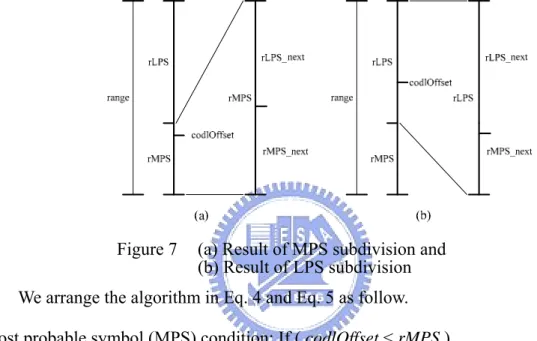
It is needed to define the initial range and the MPS probability ρ_MPS when starting the binary arithmetic decode. The value of codlOffset is composed of the bit-stream and compared with rMPS. The MPS and LPS conditions are unlike the definitions of the encoder. Figure 7 illustrates the subdivision of the MPS and LPS condition. If codlOffset is less than rMPS, the condition belongs to MPS. The range of the next interval is equal to rMPS. The probability of MPS (ρ ) is increased and

the bin value outputs “1”. The next value of codlOffset remains the current one. Figure 7(a) illustrates the MPS condition. If codlOffset is great than or equal to rMPS, the next interval turns into LPS. The range of the next interval is defined as rLPS. The probability of MPS (ρMPS) is decreased and the bin value outputs “0”. The meaning

of the next value of codlOffset is to subtract the rMPS from the current codlOffset. Figure 7(b) illustrates the MPS condition.

Figure 7 (a) Result of MPS subdivision and

(b) Result of LPS subdivision

We arrange the algorithm in Eq. 4 and Eq. 5 as follow. Most probable symbol (MPS) condition: If ( codlOffset < rMPS ) The bin Value = “1”

The value of the next codlOffset: codlOffsetNEXT =codlOffset

The MPS probability of the next interval:ρ_{MPS_NEXT} =ρ_MPS +ρ_Inc The range of the next interval: range_NEXT =rMPS

Inc

ρ : The increment of ρMPS. (Eq. 4)

Least probable symbol (LPS) condition: If( codlOffset >= rMPS ) The value of the next codlOffset: codlOffsetNEXT =codlOffset−rMPS

The MPS probability of the next interval:ρ_{MPS_NEXT} =ρ_MPS −ρ_Dec The range of the next interval: range_NEXT =rLPS

Dec

2.2.2.2

In Section 2.2.2.1, we introduce the basic algorithm of the binary arithmetic decoder. Although it can achieve the high compression gain, the algorithm works under the floating-point operation. The hardware complexity becomes the problem when we implement the binary arithmetic decoder. In Eq. 1, it has to compute the values of rMPS and rLPS with two multipliers and processes the next value of

codlOffset, range, and the probability by means of the floating adders and

comparators. It consumes the lots hardware cost because the multipliers and floating operations make the complex circuit. According to H.264/AVC standard [1], we adopt the low complexity algorithm to implement the CABAD circuit.

In order to improve the coding efficiency, there are three kinds of the binary arithmetic decoders in H.264/AVC system such as the normal, bypass, and termination decoding flow. We will show whole algorithms as follows.

The first algorithm is the normal decoding process which is shown in Figure 8. There are two main factors to dominate the hardware efficiency. One is the multiplier of range×ρLPS defined as rLPS and the other is the probability calculation defined

asρ_LPS. In Eq. 1, it applies one multiplier to find the range of LPS (rLPS). According to the H.264/AVC standard, the table-based method is used in place of the multiplication operation. In the normal decoding flowchart, codlRangeLPS looks up the table, rangeTabLPS, depending on two indexes such as pStateIdx and

qCodlRangeIdx. pStateIdx is defined as the probability of MPS (ρ_MPS) which gets

from the context model. qCodlRangeIdx is the quantized value of the current range (codlRange) which is separated to four parts in this table. The second factor of the improved method is to estimate the value of ρMPS. In Section 2.2.2.1, we know that

the value of ρ_MPS is increased when MPS condition happened and is decreased

be increased or decreased. The flowchart of Figure 8 also shows the table-based method to process the probability estimation. It divides into two sub-intervals such as MPS and LPS conditions. Depending on the sub-interval, it computes the next probability by the transIdxLPS table when the interval division is LPS and by the

transIdxMPS table when the interval is MPS. These two probability tables are

approximated by sixty-four quantized values indexed by the probability of the current interval.

codIOffset >= codIRange

binVal = !valMPS codIOffset = codIOffset - codIRange

codIRange = codIRangeLPS binVal = valMPS pStateIdx = transIdxMPS[pStateIdx] Yes No RenormD Done DecodeDecision (ctxIdx)

qCodIRangeIdx = (codIRange>>6) & 3 codIRangeLPS = rangeTabLPS[pStateIdx][qCodIRangeIdx]

codIRange = codIRange - codIRangeLPS

pStateIdx == 0?

valMPS = 1 - valMPS

pStateIdx = transIdxLPS[pStateIdx]

Yes

No

Figure 8 the flowchart of the normal decoding flow [1]

In the basic binary arithmetic decoder, the interval subdivision is operated under the floating-point operation. In practical implementation, this method causes the complexity of the circuit to be increased. The advanced algorithm adopts the integer operation for H.264/AVC. The value of the next range becomes smaller than the current interval. So we use the renormalization method to keep the scales of

codlRange and codlOffset. Figure 9 shows the flowchart of renormalization. The

MSB of codlRagne is equal to “0”, the value of codlRagne has to be shifted left until the current bit is equal to “1”. Depending on the shifted number of codlRagne,

codlOffset fill the bit-stream in the LSB.

Figure 9 Flowchart of renormalization [1]

The second algorithm is the bypass decoding process which is applied by the

specified syntax elements such as abs_mvd, significant_coeff_flag,

last_significant_coeff_flag, and coeff_abs_level_minus1. The probabilities of MPS

and LPS are fair, that is, both probabilities are 0.5. It is unnecessary to refer to the context model during decoding. Figure 10 shows the flowchart of the bypass decoding flow. Compared with Figure 8, the bypass decoding process doesn’t estimate the probability of the next interval. So we can’t see the probability computation in the bypass decoding. The computed codlRange doesn’t change which means that it has no renormalization in the bypass decoding. It just uses one subtraction to implement this decoding process. This algorithm is very simple, so we will use the architecture to speed up the CABAD system.

Figure 10 Flowchart of the bypass decoding flow [1] codIOffset >= codIRange binVal = 1 binVal = 0 Yes No Done DecodeTerminate RenormD codIRange = codIRange-2

Figure 11 Flowchart of the terminal decoding flow [1]

The third algorithm is the termination decoding process. Figure 11 show the flowchart of the terminal decoding flow. The terminal decoding process is very simple as well, but it has the more decoding procedure compared to the bypass decoding process. It doesn’t need the context model to refer to the probability. The value of the next codlRange is always to subtract two from the current codlRange depending on whether the subdivision condition belongs to MPS or not. The final values of codlRange and codlOffset are required to renormalize through the RenormD in this figure when it branches to the situation that codlOffset is smaller than

codlRange (MPS condition). The architecture of this flowchart is composed of one

constant subtraction, one comparator, and one renormalization. The termination decoding process is used to trace if the current slice is ended. It occurs one time per macroblock process which is seldom used during all decoding processes.

The efficiency, therefore, affects slightly in CABAD system. So we will focus on the first two algorithms in this section.

2.3

Binarization decoding flow

In Section 2.3, we focus on the decoding process of the binarization. It reads the

bin string to look up the suitable syntax elements. For H.264/AVC, CABAD adopts

five kinds of the binarization methods to decode all syntax elements. This section is organized as follows. In Section 2.3.1, the decoding flow of the unary code is shown at the first. The unary code is the basic coding method. Section 2.3.2 shows the truncated unary code which is the advanced unary coding method. It is applied in order to save the unary bit to express the current value. In Section 2.3.3, we introduce the fixed-length decoding flow. It is the typical binary integer method. Section 2.3.4 is the Exp-Golomb decoding flow. The Exp-Golomb decoding flow is only used for the residual data and the motion vector difference (mvd). Section 2.3.5 is the special definition by means of the table method. Specifically, we focus on the binary tree of the macroblock type (mb_type) and the sub-macroblock type (sub_mb_type).

2.3.1 Unary decoding flow (U)

Table 1 is the format of the typical unary code. If the syntax element is equal to “0”, the bin outputs single bit “0”. Besides the syntax element “0”, the bin string sends numSE “1” and one “0” in the end of the binary value. The value of numSE is equal to the syntax element. We find, therefore, the string length of the current syntax element bin string is numSE+1.

According to the unary bin string format shown above, we arrange the decoding algorithm in Eq. 6. This equation represents the pseudo code of the unary decoding flow. It sets binIdx to zero at the initial step where binIdx is the index of the bin string in Table 1. The while loop in Eq. 6 checks the current bin assigned by binIdx from the

equal to “0”, the binarization process arrives at the end of decoding step. binIdx sends to SEVal which is defined as the value of the syntax element.

Table 1 bin string of the unary code [1] Syntax

element bin string

0 0 1 1 0 2 1 1 0 3 1 1 1 0 4 1 1 1 1 0 5 1 1 1 1 1 0 … …… binIdx 0 1 2 3 4 5

Start unary decoder process

binIdx = 0 ;

while (bin[binIdx] == 1){

binIdx = binIdx + 1 ;

}

SEVal = binIdx ; (Eq. 6)

2.3.2 Truncated unary decoding flow (TU)

The truncated unary decoding flow is based on the unary one and has an additional factor of cMax which is defined as the maximum length of the current bin string. If the value of syntax element (SEVal) is less than cMax, the truncated unary and the typical unary decoding flow are the same. If SEVal is equal to cMax, the number “1” of the bin string is equal to cMax and there is no “0” bit in the current string. For example, SEVal (=“3”) is assumed. If the value of cMax is “4”, the result of bin string is equal to “1110”. If the value of cMax is “3”, the result of bin string is equal to “111” where the end bit of “0” is truncated in this case.

Start unary decoder process

binIdx = 0 ;

while (bin[binIdx] == 1 && (binIdx<cMax)){

binIdx = binIdx + 1 ;

}

SEVal = binIdx ; (Eq. 7)

Eq. 7 is the truncated unary decoding flow which is modified from Eq. 6. Besides checking the bin value, it also deals with cMax. If binIdx is less than cMax, it works the unary decoding flow. If binIdx isn’t less than cMax, it completes the decoding action until reading the end bin of “0” bit.

2.3.3 Fixed-length decoding flow (FL)

The fixed-length code is the simple-defined format of the binarization decoding process which is defined as the typical unsigned integer. The coding rule is represented by means of the typical binary number. For example, the value of “410” is

equal to “1002”. The value of “410” is defined as the decimal style and the value of

“1002” is the binary format which is the required fixed-length code.

Table 2 bin string of the fixed-length code Syntax

element bin string

0 0 0 0 0 0 0 1 0 0 0 0 0 1 2 0 0 0 0 1 0 3 0 0 0 0 1 1 4 0 0 0 1 0 0 5 0 0 0 1 0 1 … binIdx 0 1 2 3 4 5

The fixed-length decoding flow has to refer to the value of cMax which defines the number size of the current syntax element. Table 2 shows the fixed-length code definition. In this table, the cMax equals five because the maximum value of binIdx is five. All syntax elements which are decoded by the fixed-length format are always represented with six binary bits.

2.3.4

Unary/k-th order Exp-Golomb decoding flow (UEGk)

The unary/k-th order Exp-Golomb (UEGk) code is composed of two parts which are the prefix and suffix ones. The prefix part of UEGk is specified by using the truncated unary code. So the prefix part is dominated by cMax. The suffix part of this code doesn’t always apply because isn’t adopted by two cases. Both cases check the value of the provided signedValFlag and the bin string. If signedValFlag is equal to “1” and the prefix bin contains only one “0” bit, the value of syntax element is just decided by prefix bin string with the truncated unary code. If signedValFlag is equal to “0” and the prefix bin string isn’t equal to the bit string which is composed of the string length cMax of bit “1”, the decoding flow doesn’t also enter the suffix decoding step. Besides these two cases, the decoding process has to go to the suffix decoding. Eq 8 shows the suffix part algorithm by means of the pseudo code. The initial value of k is defined as the order of the unary Exp-Golomb coding which are named as UEGk. In the binarization decoding engine of CABAD, it only applies two decoding flows such as UEG0 and UEG3. UEG0 is used by the residual data decoding process and UEG3 is used by the motion vector difference one.

if( Abs( synElVal ) >= uCoff ) { sufS = Abs( synElVal ) − uCoff stopLoop = 0 do { if( sufS >= ( 1 << k ) ) { put( 1 ) sufS = sufS − ( 1<<k ) k++ } else { put( 0 ) while( k− − )

put( ( sufS >> k ) & 0x01 )

stopLoop = 1

}

} while( !stopLoop ) }

if( signedValFlag && synElVal ! = 0) if( synElVal > 0 )

put(0 )

else

2.3.5 Special decoding flow

All formats of the binarization decoding process are introduced above. But there is still a special decoding flow which we don’t describe yet. In order to perform the higher video quality, the macroblock and sub-macroblock are divided into many kinds of types such as I, P, B, and SI slices. In the four basic types, it also sorts by variable block sizes. These two syntax elements are difficult to define by means of the aforementioned decoding flows. In H.264/AVC, it adopts the table-based method to define the macro and sub-macroblock types.

Table 9-26 and Table 9-27 in the standard [1] show the macroblock types in I, SI, P, SP, and B slices. Table 9-28 in th standard [1] shows the sub-macroblock types in P, SP, and B slices. The binarization engine reads the bin string and checks if the bin string is mapped the specified location in these table. If the assigned bin string is found in the tables, it can look up the current macroblock type. We observe that the probability of the macroblock type appearance is larger and the described bin string is shorter. For example, if the value of bin string is equal to”100001” in I slice, the mapped macroblock type is equal to “2” by looking up Table 9-27 of the standard [1].

The macroblock in SI slice is the enhanced format of the macroblock type in I slice. The bin string of the SI slice macroblock type is composed of two parts: prefix bit and the suffix part. If the prefix bit is equal to “0”, it doesn’t need the suffix part and the syntax element is equal to “0”. If the prefix bit is equal to “1”, the suffix part is defined in Table9-27 of the standard [1] which mapped value of the macroblock type has to be added by “1” in SI slice.

Besides the macroblock type in SI slice, there are still two cases to process the bin value through the suffix. Table 9-27 of the standard [1] is the prefix definitions of

mbType. The suffix parts are decoded by the formats in Table 9-26 of the standard [1]

of the macroblock type in the last fields in P and B slice have to be added by the offset value. In the P and SP slices, the value of mbType is equal to the summation of the offset value “5” through Table 9-27 in the standard [1] and the bin string assignment in Table 9-26 of the standard [1] if the prefix bit is equal to “1”. In the B slices, the value of mbType is equal to the summation of the offset value “23” through Table 9-27 in the standard [1] and the bin string assignment in Table 9-26 of the standard [1] if the prefix bin string is equal to “111101”.

2.4

Context model organization

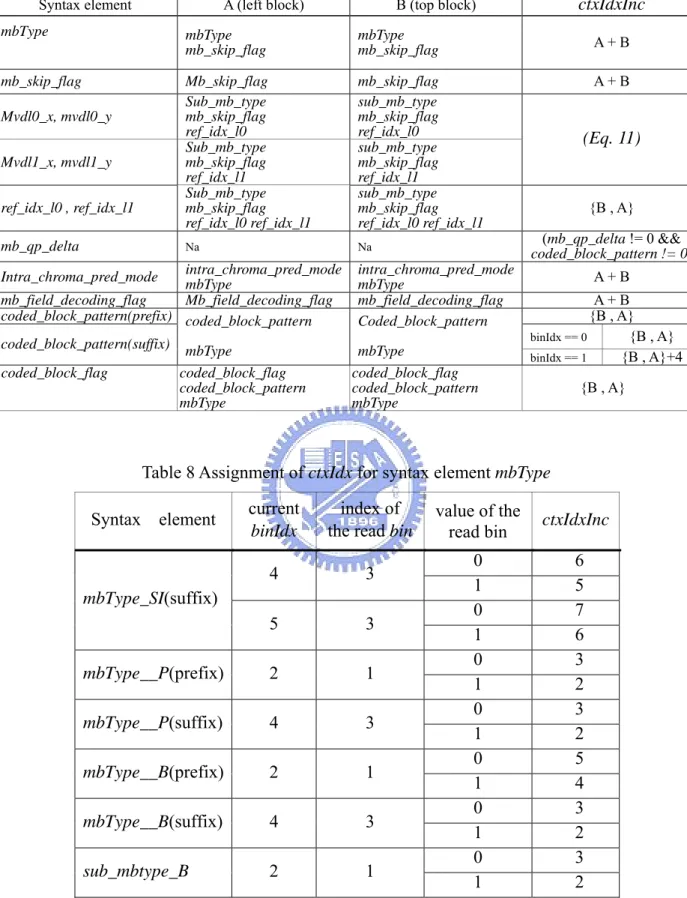
The values of the context model offer the probability value of MPS (pStateIdx) and the historical value of bin (MPS) in order to achieve the adaptive performance. In the normal decoding process of the arithmetic decoder, we have to prepare the 399 locations of the context model to record all decoding results.

context model index = ctxIdxOffset+ctxIdxInc (Eq. 9)

context model index = ctxIdxOffset+ ctxIdxBlockCatOffset+ ctxIdxInc (Eq. 10)

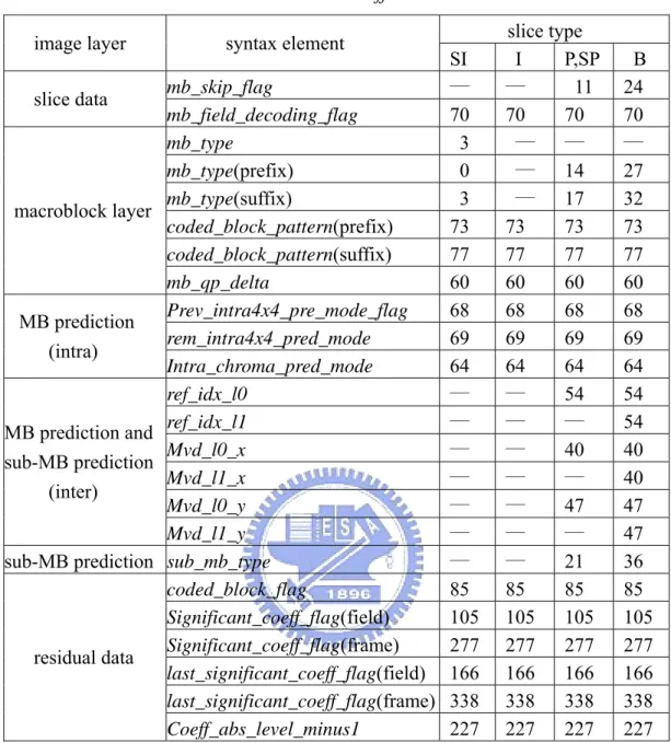
We divide into two kinds of the context model index methods to allocate the context model. Eq. 9 is one of the index methods. Besides residual data decoding, the context model index is equal to the sum of ctxIdxOffset and ctxIdxInc. Depending on the syntax element and the slice type, we can find the value of ctxIdxOffset in Table 3. The value of ctxIdxInc is looked up in Table 6 by referring to the syntax element and

binIdx. In table 6, the alphabet of “na” denotes the never happened issue and the word

of “Terminate” means that the decoding flow enters the terminal decoding process. If the generated bin is equal to “1”, the slice has to be stopped and decodes the next slice. Table 6 in Table 7 shows the value of ctxIdxInc referring to the required neighbor syntax elements of top and left blocks which will be explained in Section 2.5. Table 8 shows the value of ctxIdxInc in special binIdx when decoding mb_type in Table 6.

syntax element of the residual data decoding flow such as coded_block_flag,

significant_coeff_flag, last_significant_coeff_flag, and coeff_abs_level_minus1. The

value of the context model index is the sum of ctxIdxOffset, ctxIdxBlockCatOffset, and ctxIdxInc. The assignment of ctxIdxOffset is also shown in Table 3. The value of

ctxIdxBlockCatOffset is defined as Table 5 which is dominated by the parameters of

syntax elements and ctxBlockCat. The value of ctxBlockCat is the block categories for the different coefficient presentations. maxNumCoeff means the required coefficient number of the current ctxBlockCat. ctxBlockCat sorts five block categories which are luma_DC for 4x4 blocks, luma_AC for 4x4 blocks, luma_4x4, chroma_DC, and chroma_AC in Table 4. The value of ctxIdxInc in residual data is defined as the scanning position that ranges from 0 to “maxNumCoeff – 2” in Table 4. The scanning position of the residual data process has two scanning orders. One is scanned for frame coded blocks with zig-zag scan and the other is scanned for field coded blocks with field scan.

Table 3 Value of ctxIdxOffset definition

slice type

image layer syntax element

SI I P,SP B mb_skip_flag ─ ─ 11 24 slice data mb_field_decoding_flag 70 70 70 70 mb_type 3 ─ ─ ─ mb_type(prefix) 0 ─ 14 27 mb_type(suffix) 3 ─ 17 32 coded_block_pattern(prefix) 73 73 73 73 coded_block_pattern(suffix) 77 77 77 77 macroblock layer mb_qp_delta 60 60 60 60 Prev_intra4x4_pre_mode_flag 68 68 68 68 rem_intra4x4_pred_mode 69 69 69 69 MB prediction (intra) Intra_chroma_pred_mode 64 64 64 64 ref_idx_l0 ─ ─ 54 54 ref_idx_l1 ─ ─ ─ 54 Mvd_l0_x ─ ─ 40 40 Mvd_l1_x ─ ─ ─ 40 Mvd_l0_y ─ ─ 47 47 MB prediction and sub-MB prediction (inter) Mvd_l1_y ─ ─ ─ 47

sub-MB prediction sub_mb_type ─ ─ 21 36

coded_block_flag 85 85 85 85 Significant_coeff_flag(field) 105 105 105 105 Significant_coeff_flag(frame) 277 277 277 277 last_significant_coeff_flag(field) 166 166 166 166 last_significant_coeff_flag(frame) 338 338 338 338 residual data Coeff_abs_level_minus1 227 227 227 227

Table 4 Assignment of ctxBlockCat due to coefficient type [1] coefficient type maxNumCoeff ctxBlockCat

luma DC 16 0

luma AC 15 1

Luma coefficient 16 2

chroma DC 4 3

Table 5 Assignment of ctxIdxBlockCatOffset due to

ctxBlockCat and syntax elements of the residual data [1]

ctxBlockCat Syntax element of the residualdata _{0 1 2 3 4} coded_block_flag 0 4 8 12 16 Significant_coeff_flag 0 15 29 44 47 last_significant_coeff_flag 0 15 29 44 47 coeff_abs_level_minus1 0 10 20 30 39

Table 6 Definition of the ctxIdxInc value for context model index [1] binIdx

Syntax element

0 1 2 3 4 5 >= 6

mbType_SI(prefix) Na Na Na na na Na

mbType_SI(suffix)

mbType_I Terminate 3 4 Table 12 Table 12 7

Mb_skip_flag_P

Table 11

Na Na Na na na Na

mbType_P(prefix) 0 1 Table 12 Na na na na

mbType_P(suffix) 0 Terminate 1 2 Table 12 3 3

sub_mb_type_P 0 1 2 Na na na na

Mb_skip_flag_B Na Na Na na na na

mbType_B(prefix) Table 11 3 Table 12 5 5 5 5

mbType_B(suffix) 0 Terminate 1 2 Table 12 3 3

sub_mbType_B 0 1 Table 12 3 3 3 na mvdl0_x, mvdl1_x 3 4 5 6 6 6 mvdl0_y, mvdl1_y 3 4 5 6 6 6 Ref_idx_l0 , ref_idx_l1 4 5 5 5 5 5 Mb_qp_delta 2 3 3 3 3 3 intra_chroma_pred_mode Table 11 3 3 Na na na na prev_intra4x4_pre_mode_flag 0 Na Na na na na na rem_intra4x4_pred_mode 0 0 0 na na na Na Mb_field_decoding_flag Na Na na na na Na

coded_block_pattern(prefix) Table 11 Table 11 Table 11 na na Na

coded_block_pattern(suffix)

Table 11

Table 11 Na na na na Na

Table 7 Required syntax elements of the left and top neighbor blocks and the computation for ctxIdxInc

Syntax element A (left block) B (top block) ctxIdxInc

mbType _mbType

mb_skip_flag

mbType

mb_skip_flag A + B

mb_skip_flag Mb_skip_flag mb_skip_flag A + B

Mvdl0_x, mvdl0_y Sub_mb_type mb_skip_flag ref_idx_l0 sub_mb_type mb_skip_flag ref_idx_l0 Mvdl1_x, mvdl1_y Sub_mb_type mb_skip_flag ref_idx_l1 sub_mb_type mb_skip_flag ref_idx_l1 (Eq. 11) ref_idx_l0 , ref_idx_l1 Sub_mb_type mb_skip_flag ref_idx_l0 ref_idx_l1 sub_mb_type mb_skip_flag ref_idx_l0 ref_idx_l1 {B , A}

mb_qp_delta Na Na (mb_qp_delta != 0 &&

coded_block_pattern != 0) Intra_chroma_pred_mode intra_chroma_pred_mode_mbType intra_chroma_pred_mode_mbType A + B

mb_field_decoding_flag Mb_field_decoding_flag mb_field_decoding_flag A + B

coded_block_pattern(prefix) {B , A} binIdx == 0 {B , A} coded_block_pattern(suffix) coded_block_pattern mbType Coded_block_pattern

mbType _{binIdx == 1 {B , A}+4}

coded_block_flag coded_block_flag coded_block_pattern mbType coded_block_flag coded_block_pattern mbType {B , A}

Table 8 Assignment of ctxIdx for syntax element mbType

Syntax element current

binIdx

index of

the read bin value of the read bin ctxIdxInc

0 6 4 3 1 5 0 7 mbType_SI(suffix) 5 3 1 6 0 3 mbType__P(prefix) 2 1 1 2 0 3 mbType__P(suffix) 4 3 1 2 0 5 mbType__B(prefix) 2 1 1 4 0 3 mbType__B(suffix) 4 3 1 2 0 3 sub_mbtype_B 2 1 1 2 In addition, ctxIdxInc related to the syntax element of mvd has the special definition. Eq. 11 shows the ctxIdxInc definition of mvd. It checks the sum of the absolute mvd values in left and top sub-macroblocks. If the summation is less than “3”,

the value ctxIdxInc is defined as “0”. If the summation is greater than “32”, the value

ctxIdxInc is defined as “2”. Otherwise, the value ctxIdxInc is defined as “1”.

sum_A_B = abs(mvd[A])+ abs(mvd[B]) If ( sum_A_B < 3)

ctxIdxInc = 0 ;

else if( sum_A_B > 32) ctxIdxInc = 2 ;

else

ctxIdxInc = 1 ; (Eq. 11)

2.5

Syntax elements for the neighbor blocks

In the previous section, we have explained the methods to compute the context model index to offer the arithmetic decoder to produce the bin value. In both the residual data and the general decoding, the context model index is dominated by two factors such as ctxIdxOffset and ctxIdxInc. ctxIdxInc is only one factor related with the syntax elements of the neighbor blocks. In Table 7, we observe the variable syntax elements referring to the left and top blocks to define the ctxIdxInc of the first binIdx such as mbType, mb_skip_flag, ref_idx, mb_qp_delta, intra_chroma_pred_mode,

mb_field_decoding_flag, and coded_block_pattern. In this section, we introduce how

to refer to syntax elements of the left and top neighbor blocks.

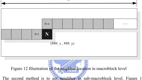
In CABAD system, it has two side syntax elements to be required such as the left and top ones. The referring position is based on the current block which can treat as not only the macroblock but also the sub-macroblock. So we have two methods to allocate the required blocks in two levels as follows.

The first method is to get neighbor in macroblock level. Figure 12 illustrates the left and top macroblocks of the current one. “N” denotes the number of the

macroblock in the current slice. The black block is the current decoding macroblock which is the N-th decoded macroblock coordinated as (MB_x , MB_y) in this slice. The macroblock “N-1” is the left macroblock and “N-w” is the top block where “w” is the width of this frame and means that the frame has “w” macroblocks in every row. In the method of Figure 12, the syntax elements are described for one parameter each macroblock except mvd, ref_idx, and residual data.

Figure 12 Illustration of the neighbor location in macroblock level

The second method is to get neighbor in sub-macroblock level. Figure 13 illustrates the sub-macroblocks in the current, left and top side macroblocks. The coordination of the current sub-macroblock is defined as (sub_MB_x , sub_MB_y). The neighbor location is like the allocation in macroblock level. If sub_MB_x is not equal to “0”, the left sub_macroblock is in the left side of the current macroblock. If sub_MB_x is equal to “0”, the left sub_macroblock can’t be found in the current macroblock and has to refer to the left side of the macroblock A. The gray circles in the macroblock A are the required sub-macroblocks which mean the syntax elements of the sub-macroblock 3, 7, 11, 15 have to be stored in order to record the left sub-macroblock. If sub_MB_y is not equal to “0”, the top sub_macroblock is in the upper side of the current macroblock. If sub_MB_y is equal to “0”, the top sub_macroblock can’t be found in the current macroblock and has to refer to the

upper side of the macroblock B. The gray circles in the macroblock B are the required sub-macroblocks which mean the syntax elements of the sub-macroblock 12, 13, 14, 15 have to be stored in order to record the top sub-macroblock.

Figure 13 illustration of the neighbor location for sub-macroblock level

2.6

Summary

In this chapter, we focus on the algorithm introduction of CABAD system. We have introduced the three kinds of the binary arithmetic decoding flows in the first decoding layer through the basic arithmetic decoding algorithm. Then, the binarization decoding flow has been depicted to generate the current syntax elements including mbType, coded_block_pattern, mvd, residual data, and so on. This is the second layer decoding flow in CABAD. The CABAD system is composed of the two layer hierarchy decoding architectures. To provide the high compression gain and the better performance, we also offer how to address the adaptive context model depending on the value of binIdx has been shown in this chapter. Based on the context model index, the required syntax elements of the neighbor blocks are defined in the previous section.

After the introduction of the CABAD system behavior, the hardware implementation will be proposed in Chapter 3 and 4. It includes the binary arithmetic

Chapter 3

Binary Arithmetic Decoder Engine

In this chapter, we propose our hardware architecture of the present design. And we will show some data to analyze the efficiency.

In H.264/AVC system, the entropy coding includes the variable length coding (UVLC and CAVLC) and CABAC. In baseline profile, UVLD and CAVLD are the main decoders to de-compress the macroblock information related to the parameter and the pixel coefficients. In main profile, CABAD substitutes for UVLD and CAVLD to restore the video data.

CABAD applies two level hierarchical decoding flows. The second level is the binarization decoding flow which is similar to the process of the variable length decoders such as UVLD and CAVLD. Besides looking for the context model index, the algorithm of the binarization is easy to realize. The first level is the arithmetic decoding flow. This decoding flow has the highly data dependency between the current interval and the next one due to make the high de-compression gain. It is, therefore, hard to accelerate this hierarchical decoding flow. The cycle count of CABAD is worse than CAVLD. So we focus on the throughput promotion in the current design.

This chapter is organized as follows. In Section 3.1, we present the overview of H.264/AVC for CABAD, and show the consideration of the two level decoding processes. In Section 3.2, an in-depth discussion of the proposed architecture of the arithmetic decoder will be given. We will propose three methods to improve the performance of our design. In Section 3.3, the binarization engine is realized by

machine of the binarization.

3.1 Overview of CABAD

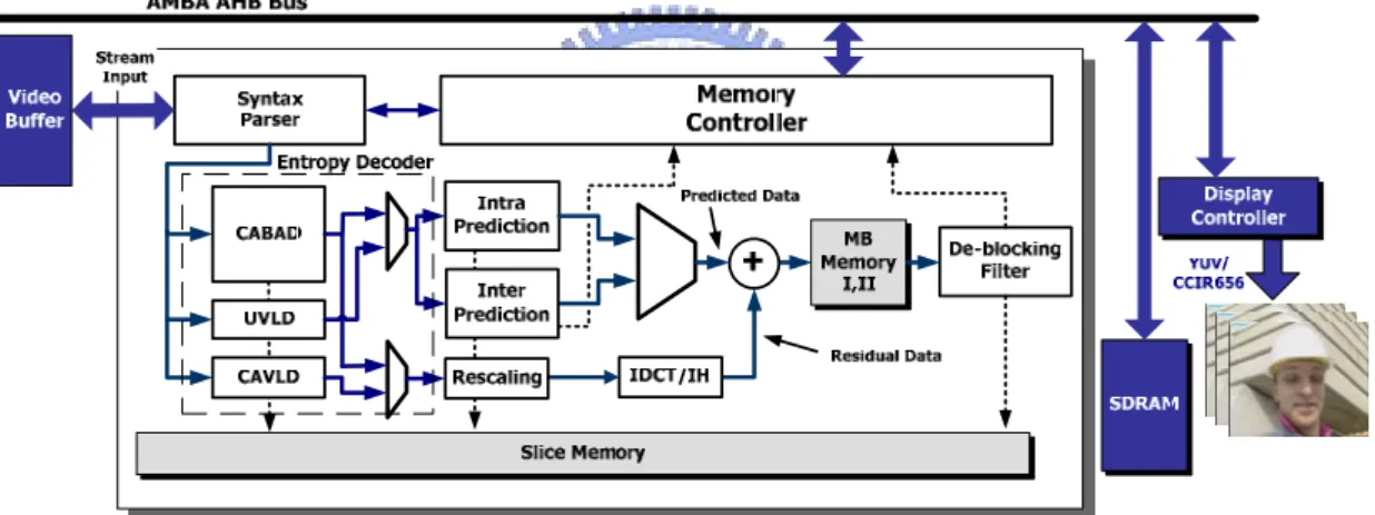
In our system, CABAD consists of three main modules namely the arithmetic decoder (AD), the binarization engine, and the SRAM module. AD is the computationally-intensive, so we focus on enhancing its efficiency.

Figure 14. System architecture of CABAD

Figure 14 is the system architecture of CABAD. The entire decoding procedure is described as follows. When starting to decode, it has to initialize the context model SRAM (399x7 bits) by looking up the initial table which is implemented by means of the combinational circuit. AD reads bit-stream to get the bin value. At the same time, it refers to the current probability from the context model SRAM to find the sub-range of MPS and LPS and updates the probability to the location of the current context model index (ctxIdx). Due to the concatenate AD execution, the several bin values form the bin string. The binarization engine reads bin string until matching the bin definition of the standard [1] and turns it into the mapped syntax element (SE) such as the macroblock parameter, mvd, residual data, and so on. We store the SE value in the SE buffer (SEB) and backup the essential SE from the SE buffer to the row-storage

(RS) SRAM (120x208 bits) which is applied to record the neighbour information when completing the macroblock decoding.

AG1 generates the address of the row-storage SRAM. We will discuss it in Chapter 4. AG2 generates the address of the context model SRAM which has been defined in Section 2.4.

We rearrange the CABAD decoding flow. Figure 15 is the flow chart of the CABAD decoding flow. At the beginning, the entire probabilities of the context model SRAM have to be initialized by the context model initial table. The context model also has to be re-initialized when the new slice starts. In Figure 15, it has two decoding flows among the dotted lines. The first decoding flow is the arithmetic decoder which is the first stage of decoding one syntax element. It produces the bin value depending on the current range (codlRange) and the current value (codlOffset). The second decoding flow is the binarization engine. It reads the bin values to judge if the bin string forms the meaningful data. If not, the binarization engine requests the arithmetic decoder to decode one bin again and re-judges the bin string until identifying the value of the current syntax element. If completing the current slice, codlRange is assigned to “51210” and codlOffset is refilled in 9-bit bit-stream from the

Figure 15 Flow chart of the CABAD decoding flow [1]

1st level decoding flow

3.2 1

st

Decoding Flow -

Architecture of the Arithmetic Decoder

The arithmetic decoder is the first level decoding flow. It de-compresses the bit-stream to the bin string which is the variable length codeword to offer the binarization engine which is the second level decoding flow turns into the SE value. The arithmetic decoder has three kinds of the decoding flows, including the normal, bypass, and terminal decoding flows. An in-depth discussion of the proposed architecture will be given.

3.2.1 Normal decoding flow

The normal decoding flow occupies 84% of the usage in the entire number of the AD demand, as shown in the pie chart of Figure 16. It is the highest usage in these three ADs. So it is easy to promote the process efficiency to focus on the normal decoding flow.

Figure 16. Percentage of the AD usage

The normal decoding flow refers to the probabilities and the historical bin value to produce the current bin. The architecture is shown as follows.

Because AD has the property of the data dependency between the current and previous intervals, the bottleneck of the process cycle is sensitive to the implementation architecture. Thus, we propose the pipeline organization to overcome the speed problem.

As shown in Figure 17, we divide the normal decoding flow into two stages which is shown as follows.

1

stage

The first stage is to read the context model. Because the normal decoding flow has to refer the context model to generate the bin string, it must add this stage to request the context model SRAM to load the current probability depending on the SE type and the bin index (binIdx). We implement the context model with the two-port SRAM so that both storing and loading of the context model can be done at the same cycle.

Figure 17. Pipeline schedule of the normal decoding flow

2

stage

The second stage is the sub-division behavior. Figure 18 is the hardware architecture of the three decoding flows. In this section, we discuss the architecture of the normal decoding flow first. We construct AD by means of the combinational circuit except L1 and L2 pre-load caches, and divide the AD decoding flow into two parts. The first part is the AD kernel. When executing the normal decoding flow, the AD kernel estimates the probability of the next interval and the current range of LPS and MPS by means of RangTabLPS, tranIdxMPS, and tranIdxLPS which are made by the hardwire.

AD kernel:

1. bypass decoding process 2. normal decoding process 3. terminal decoding process ( combinational circuit )

Renormalization Arbiter(RA) ( combinational circuit ) Pre- Load Cache

(L2) Pre- Load Cache

(L1) bit stream

codlRange codlOffset codlRange_in codlOffset_in

Control load signal and shift number

Context RangTabLPS ( combinational circuit) tranIdxMPS ( combinational circuit) tranIdxLPS (combinational circuit )

Context mode _in 8 10 9 7 mode_out codlRange_out codlOffset_out Skip renormalization bin 7 1 10 9

Figure 18. Hardware architecture of AD

Table 9 Truth table of the shift number definition related to codlRange codlRange[8:0]

Bit 8 Bit 7 bit 6 bit 5 bit 4 bit 3 bit2 bit1 bit 0

Number of Shift 1 X x x x x x x x 0 0 1 x x x x x x x 1 0 0 1 x x x x x x 2 0 0 0 1 x x x x x 3 0 0 0 0 1 x x x x 4 0 0 0 0 0 1 x x x 5 0 0 0 0 0 0 1 x x 6 0 0 0 0 0 0 0 1 x 7 0 0 0 0 0 0 0 0 1 8

The second part is the renormalization arbiter and the pre-load cache. We adopt the 2-level pre-load cache and the renormalization arbiter to avoid the waiting time of the bit-stream loading. The renormalization arbiter detects the value of codlRange if it is larger than “010016”, and generates the shift number of codlRange. The shift number

is also the required number of the bit-stream which codlOffset needs to fill in. Table 9 shows the shift number of all possible cases. As a result, the MSB of codlRange must be ‘1’.

After detecting the shift number, codlRange can be obtained and codlOffset fills in enough bit-stream by means of the renormalization arbiter. We propose 2-level pre-load cache to provide the sufficient bit-stream which the renormalization arbiter requires.

We meet three cases relating to provide the bit-stream as follows.

In the first case, there is no need to provide any bit-stream, so the L1 cache offers nothing.

Figure 19 Example of the second case

The second case is the general one if the current index of the L1 cache is greater than or equal to the shift number. The renormalization arbiter fetches the necessary bit-stream only from the L1 cache. Figure 19 is the example of the second case.

Assumed the current index of the L1 cache locates at bit 5, and the shift number of the renormalization arbiter is equal to five, which means that the 5-bit bit-stream of L1 cache is available. Renormalization Arbiter 7 6 5 4 2 1 0 7 6 5 4 2 1 0 3 3 bit-stream SRAM

{ codlOffset [4:0] , fill 5bit from pre- load cache} L 2 cache L 1 cache 8 Shift = 5 Done 8

Mapping control signal = 1

Current index Next Index

Figure 20. Example of the third case

The third case has to borrow the bit-stream from L2 cache if the current index of the L1 cache is less than the shift number. The renormalization arbiter fetches the required bit-stream not only from the L1 cache but also from the L2 cache. The mapping control signal is asserted at the same time. The content of the L2 cache is sent to L1 cache and L2 cache loads the new bit-stream from the bit-stream SRAM by means of reading the mapping control signal. Figure 20 shows the example of the third case. Assumed the current index of the L1 cache locates at bit 2, and the shift number of the renormalization arbiter is equal to five, which means that the L1 cache can provide only 3-bit bit-stream and the renormalization arbiter reads the extra bit-stream from the L2 cache. The third case prevents the loading miss penalty when the L1 cache can’t offer enough bit-stream. The loading miss penalty means that the handshaking of loading between the renormalization arbiter and the bit-stream SRAM.

symbol of “V” denotes the required bit-stream from L1 and L2 caches. The first row of this table is the first case. It needs no bit-stream because the number of the shift is equal to “0” no matter what the index of L1 cache is. The gray regions belong to the third case. The renormalization arbiter fetches the bit-stream from both L1 and L2 caches. The other regions are the second case. It just needs to fetch the bit-stream of the L1 cache.

Thus, both the AD kernel and the renormalization arbiter share one cycle to compute one bin.

Table 10. required bit-stream from the L1 and L2 caches

L1 cache(bit) L2 cache(bit) Index of

L1 cache Number Of shift

7 6 5 4 3 2 1 0 7 6 5 4 3 2 1 0 0 1 V 2 V V 3 V V V 4 V V V V 5 V V V V V 6 V V V V V V 7 V V V V V V V 7 8 V V V V V V V V 1 V 2 V V 3 V V V 4 V V V V 5 V V V V V 6 V V V V V V 7 V V V V V V V 6 8 V V V V V V V V 1 V 2 V V 3 V V V 4 V V V V 5 V V V V V 6 V V V V V V 7 V V V V V V V 5 8 V V V V V V V V

1 _V 2 _{V V} 3 V V V 4 V V V V 5 V V V V V 6 V V V V V V 7 V V V V V V V 4 8 V V V V V V V V 1 V 2 V V 3 V V V 4 V V V V 5 V V V V V 6 V V V V V V 7 V V V V V V V 3 8 V V V V V V V V 1 V 2 V V 3 V V V 4 V V V V 5 V V V V V 6 V V V V V V 7 V V V V V V V 2 8 V V V V V V V V 1 V 2 V V 3 V V V 4 V V V V 5 V V V V V 6 V V V V V V 7 V V V V V V V 1 8 V V V V V V V V 1 V 2 V V 3 V V V 4 V V V V 5 V V V V V 6 V V V V V V 7 V V V V V V V 0 8 V V V V V V V V

We divide the normal decoding of AD into two stages which have been shown in Figure 17. The first stage is to read the context model SRAM. The second stage is to decode the bit-stream into bin, and write the probability back to the context model SRAM. We apply the two stages to schedule the pipeline organization.

cycle 2 cycle 1 cycle 3 without pipeline pipeline AD operation write context model AD operation write context model AD operation write context model AD operation write context model read context model read context model read context model read context model context model index

Figure 21 timing diagram of the pipeline comparison

Figure 21 shows the timing diagram of the pipeline comparison for the normal decoding in AD. Every cycle, the current bin is made by the AD operation of the second stage and the current context model is written back to the write port of the current context SRAM, and the next context model is read from the read port of the context model SRAM. The read-port index of the context model SRAM is looked up depending on the current division condition. It can be found that the schedule without pipelining produces one bin every 2 cycles, and the other one with pipelining produces one bin every 1 cycle in average. Compared with the non-pipeline organization, the normal decoding flow with the pipeline can save the process cycle about 50%.

Besides, it is difficult to produce more than one bin per cycle for the architecture of two normal decoding of AD parallel connections due to the data dependency