正交分頻多工系統中的IQ不平衡效應與載波頻率偏移的聯合偵測與補償之研究

全文

(1)國立交通大學資訊工程學系碩士班碩士論文. 正交分頻多工系統中的IQ不平衡效應與載波頻率偏移的聯合偵測與補償之研究. Joint Estimation and Compensation of I/Q Mismatch and Carrier Frequency Offset in OFDM Systems. 研究生 : 孫明福. Student: Ming-Fu Sun. 指導教授 : 許騰尹博士. Advisor: Dr. Terng-Yin Hsu. 中華民國九十四年七月.

(2) 正交分頻多工系統中的IQ不平衡效應與載波頻率偏移的聯合偵測與補償之研究 Joint Estimation and Compensation of I/Q Mismatch and Carrier Frequency Offset in OFDM Systems. 研究生：孫明福. Student: Ming-Fu Sun. 指導教授：許騰尹博士. Advisor: Dr. Terng-Yin Hsu. 國立交通大學資訊工程學系碩士班碩士論文. A Thesis Submitted to Institute of Computer Science and Information Engineering College of Electrical Engineering and Computer Science National Chiao Tung University in Partial Fulfillment of the Requirements for the Degree of Master of Science in Computer Science and Information Engineering July 2005 Hsinchu, Taiwan, Republic of China. 中華民國九十四年七月.

(3) 正交分頻多工系統中的IQ不平衡效應與載波頻率偏移的聯合偵測與補償之研究研究生：孫明福. 指導教授：許騰尹博士. 國立交通大學. 電機資訊學院. 資訊工程學系碩士班. 摘要在本論文中，提出了一個結合載波頻率偏移與 IQ 不平衡效應的基頻 IQ 偵測與補償演算法。在目前已知的方法中，通常存在有下列兩種缺點：收斂速度慢以及補償範圍無法符合規格的要求。因此我們提出了一個可以偵測與補償增益錯誤 1 dB，相角錯誤 10 度與載波頻率偏移 50 ppm 在 2.4 GHz 的頻帶上的架構。在這樣的條件下，整體系統的效能存在有少於 0.8dB 封包錯誤率的設計損失並且比參考的演算法有高達 6dB 的系統效能提升。此外，一個基於虛擬載波頻率偏移技巧的載波頻率偏移演算法被提出來。此演算法適用於存在有 IQ 不平衡效應的情況下並且可以容忍 2dB 的增益錯誤與 20 度的相角錯誤在多重路徑的環境中。此演算法只利用三個連續的訓練序列來萃取載波頻率偏移的大小。從模擬的結果中，演算法的偵測錯誤量大約是 0.3 ppm 並且小於傳統載波頻率偏移偵測演算法，因此所提出的演算法有機會實現高效能的接收端。另外，我們所提出的虛擬載波頻率偏移演算法除了可以相容於傳統的演算法之外並且適合用在硬體的實現上。. i.

(4) Joint Estimation and Compensation of I/Q Mismatch and Carrier Frequency Offset in OFDM Systems Student: Ming-Fu Sun. Advisor: Dr. Terng-Yin Hsu. Institute of Computer Science and Information Engineering, National Chiao Tung University Abstract In this thesis, a baseband I/Q estimation and compensation algorithm is proposed which considers the joint effects of carrier frequency offset (CFO) and I/Q mismatch (IQ-M). Current solutions converge too slowly in the estimation, or the compensation range of gain-phase error and CFO cannot meet the required values. The proposed algorithm uses a feed-forward architecture which is able to estimate and compensate the non-ideal effect up to gain error 1 dB, phase error 10 degree, and CFO 50 ppm at carrier frequency 2.4 GHz. Under this condition, the system performance has less than 0.8 dB design loss in terms of packet error rate, and it is shown to have more than 6 dB improvement compared with the reference designs. By the way, a novel CFO estimation algorithm based on pseudo CFO (P-CFO) is developed to estimate the CFO value under the conditions of IQ-M for direct conversion structures with 2 dB gain error and 20-degree phase error in frequency selective fading channels. This algorithm only uses three consecutive training symbols to extract the CFO value with the technique of signal processing. From simulation results, it is shown that the estimation error of the proposed method is about 0.3 ppm which is smaller than the conventional method based on two-repeat preamble to achieve high performance receivers. In addition, the proposed P-CFO algorithm is also compatible with the conventional method and suitable for implementation issues.. ii.

(5) Acknowledgment This thesis describes research work I performed in the Integration System and Intellectual Property (ISIP) Lab during my graduate studies at National Chiao Tung University (NCTU). This work would not have been possible without the support of many people. I would like to express my most sincere gratitude to all those who have made this possible. First and foremost I would like to thank my advisor Dr. Terng-Yin Hsu for the advice, guidance, and funding he has provided me with. I feel honored by being able to work with him and look forward to a continued research relationship for my Ph.D. I am very grateful to Jui-Yuan Yu and the members of ISIP Lab, Shin-Lin Lo, You-Hsien Lin, Jin-Hwa Guo, Ming-Yeh Wu, Ming-Feng Shen, Hung-Chuan Lin, Chueh-An Tsai, for their support and suggestions. Finally, and most importantly, I want to thank my parents for their unconditional love and support they provide me with. It means a lot to me.. Ming-Fu Sun July 2005. iii.

(6) Contents Chinese Abstract. i. English Abstract. ii. Acknowledgment. iii. Contents. iv. List of Figures. vi. List of Tables. viii. Abbreviations. ix. Chapter 1. 1. Introduction. 1.1 Introduction. 1. 1.2. 4. Chapter 2 2.1. Thesis Outline. I/Q Mismatch for OFDM Systems. 5. Effect of I/Q Mismatch. 6. 2.2 I/Q Estimation without CFO. 12. 2.2.1 Proposed Algorithm. 12. 2.2.2 Simulation and Performance. 17. 2.3 I/Q Estimation with CFO. 21. 2.3.1 Proposed Algorithm. 21. 2.3.2 Simulation and Performance. 26. iv.

(7) 2.4 Summary. 27. Chapter 3 Frequency Synchronization. 28. 3.1. Effect of Carrier Frequency Offset. 29. 3.2. Carrier Frequency Offset Estimation. 32. 3.2.1. 3.3. Conventional Algorithm. 33. 3.2.2 Proposed P-CFO Algorithm. 35. Transmit Center Frequency Tolerance. 42. 3.4 Simulation and Performance. 43. 3.5 Implementation. 50. 3.6 Summary. 54. Chapter 4 Conclusion and Future Work 4.1. Conclusion. 55 55. 4.2 Future Work. 56. Appendix A Derivation of (2-13). 57. Appendix B Derivation of (3-16), (3-17). 59. Appendix C Fourier Transforms and Operations. 62. Appendix D System Model. 63. D.1. D.2. Introduction to IEEE802.11g. 63. D.1.1. Major Parameters of IEEE802.11g. 63. D.1.2. Frame Structure of IEEE802.11g. 65. Simulation Platform. 67. Bibliography. 69. Vita. 72. v.

(8) List of Figures Figure 2-1. OFDM receiver with IQ imbalance and CFO.. 6. Figure 2-2. 16 QAM constellation. (a)Without I/Q mismatch. 8. (b)Gain error: 1dB, Phase error: 10degree. Figure 2-3. Constellation diagrams (a) 16-QAM (b) 64-QAM.. 10. Figure 2-4. Packet error rate curve.. 11. Figure 2-5. The estimated channel response under IQ imbalance.. 13. Figure 2-6. Block diagram of the proposed method.. 16. Figure 2-7. Packet error rate of the proposed method for. 18. 64-QAM transmission. Figure 2-8. The effect of the IQ-M on channel estimation.. 19. Figure 2-9. FFT output (a) no I/Q compensation (b) with I/Q. 20. compensation. Figure 2-10 (a)The block diagram for the IQ estimation (b)The. 25. compensation blocks for IQ imbalance and CFO. Figure 2-11 The compensated result with gain error 2dB, phase. 26. error 20 degree, and CFO 50ppm. Figure 3-1. A typical OFDM system.. 30. Figure 3-2. QPSK constellation. (a)CFO: 0ppm (b)CFO: 5ppm. 31. vi.

(9) Figure 3-3. Estimated CFO vs. the exact CFO. The SNR is at. 34. 19dB and frequency offset is between 0~50ppm. Figure 3-4. Error function under different frequency offset.. 37. Figure 3-5. Inverse cosine function.. 39. Figure 3-6. The flowchart of the proposed P-CFO algorithm.. 41. Figure 3-7. Frequency offset estimation.. 44. Figure 3-8. CFO estimation by the two-repeat preamble based... 45. Figure 3-9. CFO estimation by the proposed P-CFO algorithm.. 45. Figure 3-10 Probability. density. function. of. 50ppm. CFO:. 47. (a)P-CFO algorithm (b)Two-repeat preamble based. Figure 3-11 Probability density function.. 48. Figure 3-12 Mean square error (MSE) of frequency estimation vs.. 49. SNR under different I/Q imbalance conditions with 50ppm CFO. Figure 3-13 Hardware design of P-CFO scheme.. 51. Figure 3-14 Layout of the P-CFO design.. 53. Figure D-1 PPDU frame format.. 65. Figure D-2 OFDM training structure.. 66. Figure D-3 Block diagram of simulation platform.. 68. vii.

(10) List of Tables TABLE 2-1 Required SNR for 10% PER. 11. TABLE 2-2 Required SNR for 10% PER. 17. TABLE 3-1 Simulation Parameters. 43. TABLE 3-2 Required SNR for 10-6 MSE. 49. TABLE 3-3 Complex Multiplier. 52. TABLE 3-4 The Complexity (Gate Count) of P-CFO. 52. TABLE 3-5 Chip Profile. 53. TABLE C-1 Fourier Transforms. 62. TABLE C-2 Fourier Operations. 62. TABLE D-1 Modulation Parameters. 64. TABLE D-2 Timing Related Parameters. 64. viii.

(11) Abbreviations AWGN. additive white Gaussian noise. BPSK. binary phase shift keying. CFO. carrier frequency offset. CMOS. complimentary metal-oxide-semiconductor. CRLB. Cramér-Rao lower bound. DA. data-aided. DAB. digital audio broadcasting. DFT. discrete Fourier transform. DVB-T. digital video broadcasting terrestrial TV. FFT. fast Fourier transform. GIB. guard interval based. ICI. inter-carrier interference. IFFT. inverse fast Fourier transform. I/Q. in phase/quadrature phase. IQ-M. I/Q mismatch. LO. local oscillator. MG. mirror gain. MIMO. multi-input multi-output. ML. maximum likelihood. MSE. mean square error. NDA. nondata-aided. NLS. nonlinear least squares ix.

(12) OFDM. orthogonal division frequency modulation. P-CFO. pseudo CFO. PDF. probability density function. PER. packet error rate. PHY. physical layer. PLCP. PHY convergence procedure. PPDU. PLCP protocol data unit. PSDU. PHY service data unit. QAM. quadrature amplitude modulation. QPSK. quadrature phase shift keying. RF. radio frequency. SG. signal gain. SISO. single-input single-output. SNR. signal-to-noise ration. WLAN. wireless local area network. x.

(13) Chapter 1 Introduction 1.1 Motivation Orthogonal Frequency Division Multiplexing (OFDM) is a kind of spectrally efficient signaling technique for communications over frequency selective fading channels [1], [2], which has been adopted by many transmission systems, e.g., WLAN systems based on IEEE802.11a/g [3], [4], digital audio broadcasting (DAB) [5], and digital video broadcasting terrestrial TV (DVB-T) [6]. Unfortunately, OFDM systems are sensitive to imperfect synchronization and non-ideal front-end effect, caused serious system performance degradation. It also causes strict front-end specifications and results in expensive front-end circuits. Generally, OFDM is highly sensitive to carrier frequency offset (CFO) between transmitter and receiver, which is caused by a Doppler shift of the radio frequency (RF) carrier, the mismatch of local oscillator (LO) between the transmitter and the receiver or phase noise of an oscillator. Frequency offset can introduce inter-carrier interference (ICI) in an OFDM receiver due to the loss of the orthogonality between sub-carriers and severely degrade the overall system performance if without appropriate correction. In order to prevent performance degradation, OFDM systems pay a cost of strict front-end specifications and -1-.

(14) expensive front-end implementations. Recently, some researches have focused on the development of monolithic receiver architecture, especially for low cost technology. Among of different receiver architectures, direct conversion architecture is one potential candidate for simply integration. However, direct conversion receivers are also suffered from their own impairments, such as I/Q mismatch (IQ-M) of non-ideal RF circuits, which is due to the gain and phase mismatch between in-phase (I) and quadrature-phase (Q) paths [7]-[9]. More specifically, it occurs when both phase and gain differences between I and Q are not exactly 90 degree and zero gain error. The effects of IQ-M not only introduce the unwanted image interference into the desired signal but also limit the accuracy of the CFO estimation. Practically, CFO and IQ-M will jointly occur and greatly degrade the system performance. In order to handle frequency synchronization, a number of methods for OFDM systems have been proposed which they can be divided into three categories. a) data-aided (DA). Special training symbols are inserted into the transmitted data [10], [11]. b) nondata-aided (NDA). Synchronization uses the transmitted data without any other additional information [12], [13]. c) guard interval based (GIB). Use the received data before the FFT and the inserted guard interval in the OFDM signal frame [14], [15]. Some blind frequency estimators which rely on signal statistics are also applied to accomplish frequency synchronization [16], [17]. Although these methods can work well under frequency offset, they don’t take the IQ-M into considerations, and then the estimation error will be enlarged when the IQ-M phenomenon is introduced into the system. In [18], the proposed algorithm has considered jointly CFO and IQ-M phenomenon, whose CFO tolerance is confined within the range from -47 kHz to 47 kHz, which doesn’t meet the general. -2-.

(15) requirements from -125 kHz to 125 kHz. An iteration algorithm [19] is developed, however it doesn’t guarantee the convergence condition of the estimation when the packet based WLAN standards are considered. In [20], a joint estimation of CFO, channel and IQ-M based on maximum likelihood (ML) criterion is introduced, whose accuracy almost achieves the Cramér-Rao lower bound (CRLB), but the computing cost is too high to be suitable for hardware implementation. A nonlinear least squares (NLS) frequency estimator under I/Q imbalance is proposed in [21], where it pays a cost of computational complexity for matrix operations in the NLS method. In addition, the synchronization format (training symbols) of the proposed NLS method differs from the state of art in WLAN standards such as IEEE802.11a/g. This means that the NLS method isn’t compatible with current standards. There are also many methods proposed to compensate the IQ-M so far. An I/Q correction scheme under a noisy Rayleigh fading channel is proposed in [25], but it does not take CFO effect into consideration. The correction method discussed in [18] can only compensate the IQ-M with gain error up to 0.414 dB and phase error to 10 degree, which does not reach the conventional tolerance, say gain error 1dB and phase error 10 degree. Another approach is to do the work by analog circuit [22]. Considering the joint impairments of CFO and IQ-M, first, a modified frequency offset estimation algorithm which is suitable for implementation issue is developed to overcome the large CFO estimation error caused by IQ-M. In the proposed algorithm, it uses three training symbols, which are rotated by additional frequency offset purposely, to carry out the frequency offset estimation even if there is the interference of IQ-M. Then an all-digital scheme for I/Q estimation is developed, including a robust algorithm for I/Q correction in the presence of CFO, which can tolerate CFO up to 125 kHz, 1dB gain error, and 10-degree phase error. From simulation results, it. -3-.

(16) is clear to see that the performance of the proposed scheme is better than the reference designs, thus it can achieve a high performance receiver.. 1.2 Thesis Outline After a short introduction to the effect of carrier frequency offset with IQ-M, the second chapter will present the proposed algorithm and analyze the proposed algorithm. Following that, the effect of IQ-M caused by non-ideal front end will be presented in chapter three. Chapter three will explore an algorithm to compensate the IQ-M. In practical, carrier frequency offset and IQ-M can happen jointly. Finally, this thesis is summarized in chapter four.. -4-.

(17) Chapter 2 I/Q Mismatch for OFDM Systems One of the key effects coming from non-ideal RF circuit is I/Q mismatch (IQ-M), which is due to the gain and phase mismatch between in-phase (I) and quadrature-phase (Q) channels. More specifically, it occurs when the difference of the phase in I and Q channels from local oscillator is not exactly 90 degree and the gain is not the same. In real front-end circuit, however, IQ-M and CFO will jointly occur and severely degrade the system performance. An I/Q correction scheme under a noisy Rayleigh fading channel is proposed in [25], but it does not take CFO effect into consideration. The correction method discussed in [18] can only compensate the mismatch with gain error up to 0.414 dB and phase error to 10 degree, which does not reach the conventional tolerance, say gain error 1dB and phase error 10 degree. Another approach [19], however, uses the iteration algorithm, which does not guarantee the convergence of estimation when the packet based WLAN standards are considered. Another approach is to do the work by analog circuit [22]. Here, an all-digital I/Q estimation algorithm is proposed. We first describe the IQ-M model. Then a novel scheme for I/Q estimation is developed, including a robust. -5-.

(18) algorithm for I/Q correction in the presence of CFO, which can tolerate CFO up to 125 kHz, gain error 1dB, and phase error 10 degree.. 2.1. Effect of I/Q Mismatch. I/Q imbalance arises when the signal in I and Q channels do not meet the orthogonality and the power balance. This effect can be modeled in two parameters: gain error ε and phase error ϕ . Based on the direct conversion architecture in [8], [19], and [22], the system block can be depicted as Figure 2-1.. Figure 2-1. OFDM receiver with IQ imbalance and CFO. The mathematical modeling can be derived from. rBB = I BB + jQBB = cos( Δωt ) Re{ y} − sin( Δωt ) Im{ y} + j (1 − ε ) sin( Δωt + ϕ ) Re{ y} + j (1 − ε ) cos( Δωt + ϕ ) Im{ y}. (2-1). where IBB and QBB are the baseband data in I and Q channel respectively which are distorted by IQ-M with CFO Δω induced from the front-end, and y is the coming signal in the receiver. Also, equation (2-1) can be further summarized as. -6-.

(19) rBB = ξ ⋅ y ⋅ e. j Δω t. (. +σ ⋅ y⋅e. ). jΔωt ∗. (2-2). Thus the received signal can be regarded as a gain, say Signal Gain (SG) ξ , of its original one added by the conjugate multiplied by a delta value, say Mirror Gain (MG) σ , which are given as ϕ − jϕ ε j2 ⎤ 2 SG : ξ = ⎢ (1 + )e + (1 − )e ⎥ 2 ⎣⎢ 2 2 ⎦⎥. (2-3). ϕ ϕ ε j2 ε − j2 ⎤ (1 ) e (1 ) e + − − ⎢ ⎥ 2 ⎢⎣ 2 2 ⎥⎦. (2-4). 1⎡. MG : σ =. ε. 1⎡. If neither gain nor phase error exists, MG will reduce to zero, and SG remains unit. Note that the phase rotation is inversed in the direction between the original signals and its conjugate if the CFO is present. This means the conventional compensation algorithm [10] which simply multiplies the data with an exponential term has to be modified in accordance with gain and phase errors. In OFDM systems, rBB is further transformed into frequency domain in the receiver,. RBB ,n = DFTN {rBB } = ξ ⋅ DFT { x ⋅ e jΔωt } + σ ⋅ DFT {( x ⋅ e jΔωt )∗} = ξ ⋅ Yn ⋅ ( Dn + ICI n ) + σ ⋅ Y−∗n ⋅ ( Dn∗ + ICI n∗ ). (2-5). = ξ ⋅ Yn ⋅ Cn + σ ⋅ Y−∗n ⋅ Cn∗. Yn is the sub-carrier of received signals in one DFT block, N represents the DFT point number, and –N in the footnote makes Y mirrored in block size N. Dn is the distortion due to CFO which is accompanied with inter-carrier interference ICIn [10]. If y is convolved with a multipath channel, the data in receiver baseband is Yn = Xn．Hn, where Xn and Hn denote the original baseband signals and channel response respectively.. -7-.

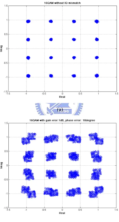
(20) The effects of IQ-M on the 16 QAM constellation after channel correction is depicted in Figure 2-2. Thus, IQ-M can limit the ability of the receiver to achieve better performance especially for high data rate, e.g., 64 QAM constellation.. (a). (b) Figure 2-2. 16 QAM constellation. (a)Without I/Q mismatch (b)Gain error: 1dB,. Phase error: 10degree. -8-.

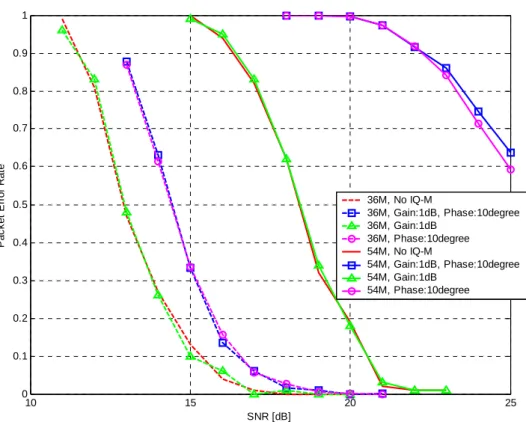
(21) There are simulation results to see how about IQ-M affects the system performance. From simulation results, it is clear to see that the phase error degrades the system performance greatly than the gain error. And the higher data rate, e.g., 54Mbps, is more sensitive to the IQ-M. This is because the minimum distance of high QAM constellation becomes smaller than low data rate. Then a serious decision error will be caused. Figure 2-3 shows the constellation diagrams for 16-QAM and 64-QAM. Figure 2-4 shows the PER curve under the IQ-M and TABLE 2-1 summarizes the required SNR for 10% PER.. -9-.

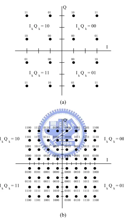
(22) Q 11. 01. 10. I Q = 10 k. I Q = 00. k. 10. 11. k. 00. k. 00. 01. I 01. 00. 00. I Q = 11 k. 11. 10. I Q = 01. k. k. 10. k. 01. 11. (a) Q. I Q = 10 k. 1000 1001 1101. 1100. 1101 1111 0111 0101. 1010 1011 1111. 1110. 1001 1011 0011 0001. 0010 0011 0111. 0110. 1000 1010 0010 0000. 0000 0001 0101. 0100. 0100 0101 0001 0000. 0000 0010 1010. 1000. 0110 0111 0011 0010. 0001 0011 1011. 1001. 1110 1111 1011 1010. 0101 0111 1111. 1101. 1100 1101 1001 1000. 0100 0110 1110. 1100. k. I Q = 11 k. 1100 1110 0110 0100. k. I Q = 00 k. I. I Q = 01. (b) Figure 2-3. Constellation diagrams (a) 16-QAM (b) 64-QAM.. - 10 -. k. k. k.

(23) TABLE 2-1. REQUIRED SNR FOR 10% PER SNR. SNR (IQ-M). (AWGN). gain. phase. gain & phase. 36Mbps. 15.3. 15. 16.6. 16.6. 54Mbps. 21. 21. N/A. N/A. 1. 0.9. 0.8. Packet Error Rate. 0.7. 0.6 36M, 36M, 36M, 36M, 54M, 54M, 54M, 54M,. 0.5. 0.4. 0.3. No IQ-M Gain:1dB, Phase:10degree Gain:1dB Phase:10degree No IQ-M Gain:1dB, Phase:10degree Gain:1dB Phase:10degree. 0.2. 0.1. 0 10. 15. 20 SNR [dB]. Figure 2-4. Packet error rate curve.. - 11 -. 25.

(24) 2.2. I/Q Estimation without CFO. 2.2.1 Proposed Algorithm Here we just analysis the effect of IQ-M in OFDM systems and propose a simple scheme to estimate IQ-M. A joint estimation of IQ-M and CFO will be developed in chapter four. If there is no CFO, equation (2-5) can be rewritten as RBB ,n = DFTN {rBB } = ξ ⋅ DFT {x} + σ ⋅ DFT {( x )∗}. (2-6). = ξ ⋅ Yn + σ ⋅ Y−∗n. Equation (2-6) shows that the IQ-M causes the symbol at the sub-carrier n to be scaled by the complex factor ξ . In addition, the complex conjugate of the symbol at sub-carrier –n multiplied by another complex factor σ will be present. Therefore the symbol at the sub-carrier n will include the unwanted interference related to the symbol at the sub-carrier –n. This means that IQ-M can distort the accuracy of received signal. After channel correction, the effect of IQ-M on channel estimation can be expressed as: R Hˆ n = BB ,n Xn = ξ ⋅ Hn + σ ⋅. - 12 -. X −∗n , N Xn. (2-7) ⋅H. ∗ −n.

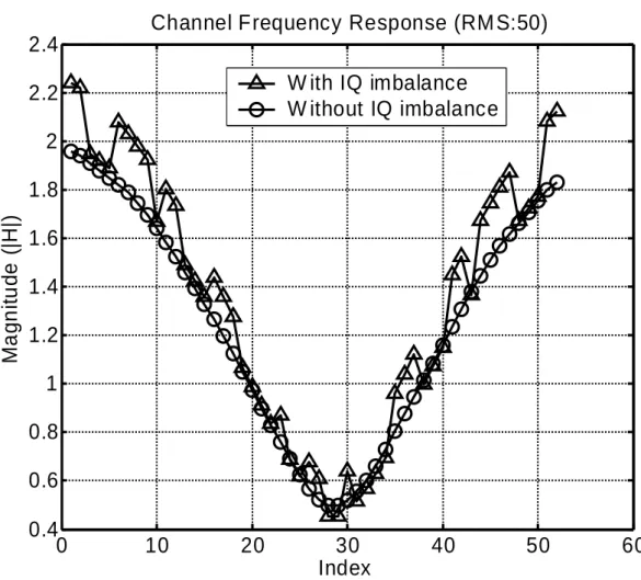
(25) where H n means the exact channel frequency response, Hˆ n is the channel frequency response calculated from long training symbol. From equation (2-7), it is obvious that IQ-M has large impact on the channel frequency response. If we use the influenced channel frequency response, the performance will be terrible especially for 64-QAM transmission. So the challenge is to find precision I/Q parameters and the exact channel frequency response at the same time. Figure 2-5 shows the channel frequency response. Note that Figure 2-5 only shows carriers 26 to 1 and -1 to -26 of FFT output.. Channel Frequency Response (RM S:50) 2.4 W ith IQ imbalance W ithout IQ imbalance. 2.2 2. Magnitude (|H|). 1.8 1.6 1.4 1.2 1 0.8 0.6 0.4 0. 10. 20. 30 Index. 40. Figure 2-5. The estimated channel response under IQ imbalance.. - 13 -. 50. 60.

(26) From Figure 2-5, the variation between sub-carriers Hˆ 26 and Hˆ 25 is very small. However there is a large difference between sub-carriers Hˆ 25 and Hˆ 24 . So the result of Hˆ 24 − Hˆ 25 can be expressed as X −*25 * X −*24 * ˆ ˆ H 24 − H 25 = ξ ⋅ ( H 24 − H 25 ) + σ ⋅ ( H −24 − H −25 ) X 24 X 25. (2-8). Because the coherency bandwidth of the channel is much larger than the inter-carrier-sapcing (channel bandwidth = 20 MHz, the bandwidth of the inter-carrier-spacing = 312.5 kHz), the variation of two consecutive channel carriers can be assumed to be very small. That means H 24 ≈ H 25 . And ξ = 0.5[1 + (1 + ε )(cos(θ ) − j sin(θ ))] ≈ 1 . Since. X −*25 X* = − −24 = −1 , Hˆ −*24 + Hˆ −*25 can be expressed as: X 25 X 24. Hˆ −*24 + Hˆ −*25 = ξ * ⋅ ( H −*24 + H −*25 ) + σ * ⋅ (. X 25 X H 25 + 24 H 24 ) X −25 X −24. = ξ * ⋅ ( H −*24 + H −*25 ) + σ * ⋅ ( H 24 − H 25 ). (2-9). ≈ H −*24 + H −*25. Using these approximations in equation (2-8) leads to. Hˆ 24 − Hˆ 25 = σ ⋅ (Hˆ −*24 + Hˆ −*25 ). (2-10). The results for the estimation of I/Q parameters are. σ = (Hˆ 24 − Hˆ 25 ) /( Hˆ −*24 + Hˆ −*25 ). (2-11). ξ = 1−σ *. (2-12). - 14 -.

(27) There are two consecutive long training symbols for channel estimation in the IEEE802.11a/g standard. After calculating I/Q parameters and the channel frequency response from long training symbol one, we can use the information to update I/Q parameters when long training symbol two is coming. And the final I/Q parameters are expressed as (see Appendix A for details). σ final =. Hˆ 2 [24] − Hˆ 2 [25]( Hˆ 1[24]/ Hˆ 1[25]) Hˆ 1*[−24] ⋅ ( X −*24 / X 24 ) − Hˆ 1*[−25] ⋅ ( X −*25 / X 25 ) ⋅ ( Hˆ 1[24]/ Hˆ 1[25]). (2-13). ξ final = 1 − σ *final. (2-14). where Hˆ 1[ k ] is the channel frequency response calculated form long training symbol one and Hˆ 2 [ k ] is the observed channel frequency response from long training symbol two. So equation (2-13) shows that I/Q parameters not only depend on the current channel frequency response but also the previous one. From Figure 2-5, there are 20 transitions in the long preamble sequence if the I/Q imbalance exists. So the proposed method will get 20 estimates of I/Q parameters. Average them and use them for compensation. The algorithm works as follows: 1) Use long training symbol one to estimate I/Q parameters and channel frequency response at the same time. 2) Use long training symbol two and channel frequency response calculated from long training symbol one to estimate the final I/Q parameters and channel frequency response. 3) Correct the incoming payload by the final I/Q parameters and channel frequency response. 4) If next packet is coming, go to 1).. - 15 -.

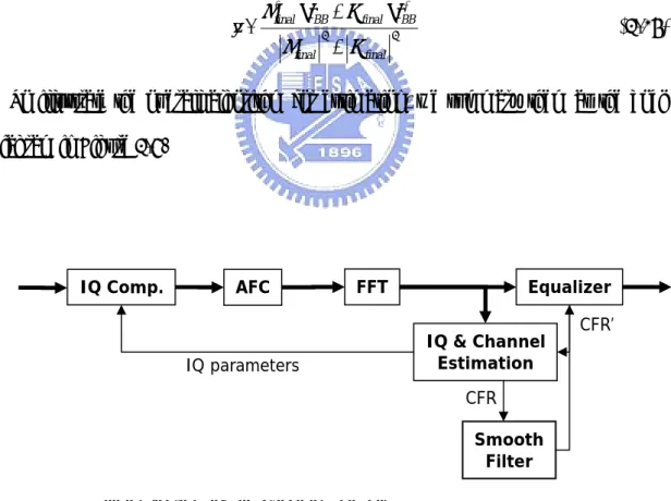
(28) The proposed method estimates the precision channel frequency response and exact IQ-M at the same time. Since I/Q parameters are static over many symbols, the influenced signal can be corrected by the estimates of the IQ-M. In this proposed method, the IQ-M is estimated in the frequency domain, but the compensation scheme of IQ-M is applied in the time domain. This means the influenced signal can be compensated in the time domain, i.e. before the FFT component. Naturally, time domain compensation is inherently better than frequency domain compensation. This is because the time domain compensation can avoid some decision errors, which are inevitable in the decision directed approach. With the mathematical derivation, the original data can be solved from. yˆ =. ∗ ξ ∗final ⋅ rBB − σ final ⋅ rBB 2. ξ final − σ final. (2-15). 2. To illustrate the overall algorithm for estimation, we summary them as the bock diagram in Figure 2-6.. IQ Comp.. FFT. AFC. Equalizer IQ & Channel Estimation. IQ parameters. CFR Smooth Filter. Figure 2-6. Block diagram of the proposed method.. - 16 -. CFR’.

(29) 2.2.2 Simulation and Performance The gain and phase imbalance were set at 1dB and 10° respectively. Four cases are considered in the simulation: (a) no I/Q imbalance. (b) estimate and compensate IQ-M by the proposed method. (c) estimate and compensate IQ-M by Ref. [26]. (d) no I/Q compensation. In Figure 2-7 the compensation scheme gets the degradation at a required SNR for 10% packet error rate (PER) down to 0.2 dB. A comparison is also shown in TABLE 2-2. From TABLE 2-2, the required SNR for 10% packet error rate of the proposed method is less than [26] about 1.3 dB. This means the proposed method can fully estimate and compensate the IQ-M. Figure 2-8 shows that the precision channel frequency response can be obtained by the proposed method. This means the proposed method can estimate the IQ-M and channel frequency response at the same time.. TABLE 2-2 REQUIRED SNR FOR 10% PER Case SNR (dB). (a)No I/Q imbalance. 23.5. (b)The proposed method. 23.7. (c)Ref. [26]. 25. (d)No I/Q compensation. N/A. - 17 -.

(30) Figure 2-7 Packet error rate of the proposed method for 64-QAM transmission.. - 18 -.

(31) Figure 2-8 The effect of the IQ-M on channel estimation.. - 19 -.

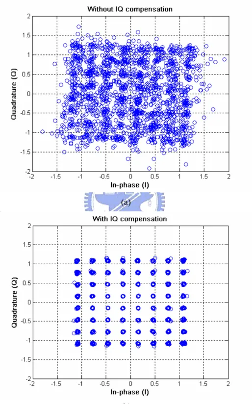
(32) In Figure 2-9 the constellation shall look more regularly if the I/Q compensation scheme is applied. It is obvious that there is a marked improvement.. (a). (b) Figure 2-9 FFT output (a) no I/Q compensation (b) with I/Q compensation.. - 20 -.

(33) 2.3. I/Q Mismatch Estimation with CFO. 2.3.1 Proposed Algorithm In this section, a joint estimation of IQ-M and CFO is developed. When estimating the effect of IQ-M, there are several parameters have to be considered jointly: estimated channel frequency response Hˆ , SG, MG, and Δω . Some WLAN standards have fixed pilot symbols for channel parameter estimation, and the sub-carrier pattern is pre-known [3], [4]. Thus, the channel frequency response can be estimated by dividing the received sub-carriers by the preamble. The result, however, will be different when IQ-M is involved, and is interfered by a conjugate and mirror of itself. Therefore, the resulting estimated channel response is then R Hˆ n = BB ,n Xn = ξ ⋅ H n ⋅ Cn + σ ⋅. X −∗n , N Xn. (2-16) ∗ −n. ⋅ H ⋅C. ∗ n. with X n ∈ {−1,+1} the preamble sub-carrier. When X n ≠ X − n , N , there is a large transition in the received channel frequency response Hˆ , and σ can be calculated with this property as illustrated in Figure 2-5. As can be seen, there are several sharp transitions, and we take the average of σ , which is estimated from those transitions, to be the Mirror Gain. The transition locations keep the same in every preamble since the pattern is pre-defined, and the relationship can be derived from equation (2-16). In the following discussion, we take n = 1 and 2 to be the reference index for algorithm derivation. Thus,. - 21 -.

(34) ∗ ⋅ C1∗ Hˆ 1 = ξ ⋅ H1 ⋅ C1 + σ ⋅ H 63 Hˆ = ξ ⋅ H ⋅ C − σ ⋅ H ∗ ⋅ C ∗ 2. 2. 2. 62. (2-17). 2. with n = 0 the DC value. Subtracting Hˆ 1 from Hˆ 2 , we’ll have an estimation of MG,. σ=. ( Hˆ 1 − Hˆ 2 ) − ξ ( H1C1 − H 2C2 ) ( H 62C2 + H 63C1 )*. (2-18). Similarly, we can find out H 62C2 and H 63C1 from equation (2-16), which are shown as H 62C2 = H 63C1 =. ∗ Hˆ 62 ⋅ C2 ⋅ C62−1 + σ ⋅ H 2∗ ⋅ C62 ⋅ C62−1 ⋅ C2. ξ. (2-19). ∗ ⋅ C63−1 ⋅ C1 Hˆ 63 ⋅ C1 ⋅ C63−1 − σ ⋅ H1∗ ⋅ C63. ξ. Substituting equation (2-19) into equation (2-18), and we can find that. σ=. ( Hˆ 1 − Hˆ 2 )ξ ∗ − ( H1C1 − H 2C2 ) ξ. 2. ∗ ∗ ⎡ ( Hˆ 62C2C62−1 + Hˆ 63C1C63−1 ) − σ ( H1∗C63 C63−1C1 − H 2∗C62 C62−1C2 ) ⎤⎦ ⎣. *. (2-20). From the above derivation, the MG changes its original behavior due to the existence of CFO. Before solving the equation for MG, we have first to reduce and simplify some terms in equation (2-20). To estimate MG and SG, we follow the proposed P-CFO scheme to multiply the received signal with an inversed rotation term. Thus equation (2-16) is then reduced to ∗ ∗ 2 RBB,n = ξ ⋅ Yn + σ ⋅ Y− n ⋅ (Cn ). (2-21). Use equation (2-21) and follow the derivation in equations (2-16) ~ (2-20), we can find that equation (2-20) becomes. - 22 -.

(35) 2 ( Hˆ n − Hˆ n +1 )ξ ∗ − ( H nCn − H n +1Cn +1 ) ξ σ= X X ( − n Hˆ − nCn∗ − − n −1 Hˆ −⋅∗n −1Cn∗+1 ) − σ ∗ ( H nC− nCn∗ − H n +1C− n −1Cn∗+1 ) Xn X n +1 (2-22) ∗ ˆ ˆ ( H n − H n +1 )ξ ≅ X −n ˆ X H − nCn∗ − − n −1 Hˆ −⋅∗n −1Cn∗+1 ) − σ ∗ ( H nC− nCn∗ − H n+1C− n−1Cn∗+1 ) ( Xn X n +1. with the reasonable assumption that the channel changes slowly in its frequency response. We also define some terms as. m = ( Hˆ − n −1 ⋅ Cn +1 + Hˆ − n ⋅ Cn )∗ n = H n ⋅ Cn∗ ⋅ C−∗n − H n +1 ⋅ Cn∗+1 ⋅ C−∗n −1 p = ( Hˆ − Hˆ ) ⋅ ξ ∗ n. (2-23). n +1. Thus we can solve MG and SG from the equation below. ⎧⎪n σ 2 − mσ + p = 0 ⎨ ∗ ⎪⎩ξ = 1 − σ. (2-24). All the parameters in equation (2-24) are complex numbers, and solution can be found by setting the real part and imaginary part to be equal to zero. Each complex number is denoted separately as x = (xR, xI) . Therefore following equations hold: ⎧(σ R2 + σ I2 )nR − (σ R mR − σ I mI ) + pR = 0 ⎨ 2 2 ⎩ (σ R + σ I )nI − (σ R mI − σ I mR ) + pI = 0. (2-25). Some parameters u, v, w are also defined first. ⎧ mR nI − nR mI 2 ) ]nR ⎪ u = [1 + ( mR nR + mI nI ⎪ ⎪⎪ 2(mR nI − nR mI )(nR pI − nI pR )nR (mR nI − nR mI )mI − mR + ⎨v= (mR nR + mI nI ) 2 mR nR + mI nI ⎪ ⎪ (n p − nI pR ) 2 nR (nR pI − nI pR )mI ⎪w = R I + + pR (mR nR + mI nI ) 2 mR nR + mI nI ⎪⎩. (2-26). Rearrange the equation (2-25) with the notation in equation (2-26), it can be easily found. - 23 -.

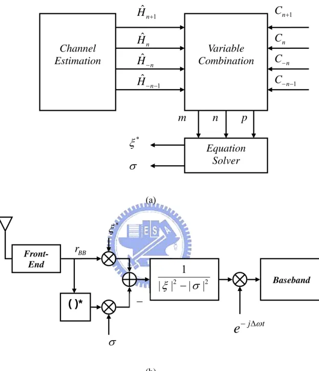
(36) uσ R2 + vσ R + w = 0. (2-27). Thus, σ R can be solved by. σR =. −v ± v 2 − 4uw 2u. (2-28). And σ I can be written as −mI ± mI 2 − 4nR (σ R2 nR − σ R mR + pR ) σI = 2nR. (2-29). Consequently, MG is found from equations (2-28) and (2-29), and SG can be solved from taking the conjugate of MG and subtracting it from one as shown in equation (2-24). Note that, however, we cannot know SG and MG in the beginning of calculation since the parameter p involves the initial SG value. According to the simulation, we can follow equations (2-23) ~ (2-29) by first setting SG to be unit. After the first calculation, we put the results into equations (2-24) ~ (2-29) and solve them again, then accurate SG and MG can be always found in five iterations. Those calculations will be done in receiving the guard interval of an OFDM symbol, and will be ready for the compensation of the coming data. With the information of estimated channel response and the existing CFO amount, we can calculate the necessary MG and SG for data compensation. The original data can be solved from equation (2-30). yˆ =. ∗ ξ ∗ ⋅ rBB − σ ⋅ rBB 2 2 ξ −σ. (2-30). To illustrate the overall algorithm for estimation and compensation algorithm, we summary them as the block diagram in Figure 2-10.. - 24 -.

(37) Channel Estimation. Hˆ n +1. Cn +1. Hˆ n. Cn. Variable Combination. Hˆ − n Hˆ − n −1. C− n C− n −1. m. ξ*. n. p. Equation Solver. σ (a). ξ* FrontEnd. rBB. 1 | ξ | − | σ |2. Baseband. 2. −. ( )*. e − j Δω t. σ (b). Figure 2-10 (a)The block diagram for the IQ estimation (b)The compensation blocks. for IQ imbalance and CFO.. - 25 -.

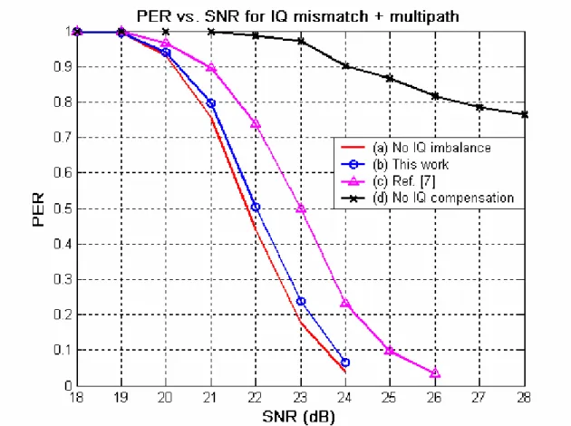
(38) 2.3.2 Simulation and Performance The simulation result is depicted for 64-QAM constellation, CFO and IQ-M. As can be seen in the simulation result, the degradation in the PER values due to the impairment such as IQ-M and CFO is significant. Figure 2-11 shows that the proposed method is also work well under CFO only. It is also shown that we achieve about 2.5dB system improvement compared with the reference designs illustrated in Figure 2-11.. Data rate:54Mbps 1 AWGN only CFO only, this work CFO only, conventional CFO&IQ-M, this work CFO, this work; IQ-M, Ref[18]. 0.9. 0.8. Packet Error Rate. 0.7. 0.6. 0.5. 0.4. 0.3. 0.2. 0.1. 0 17. 18. 19. 20. 21. 22. 23. 24. SNR [dB]. Figure 2-11 The compensated result with gain error 2dB, phase error 20 degree, and CFO 50ppm.. - 26 -.

(39) 2.4. Summary. In this chapter, an IQ-M model with CFO is investigated and the effect of IQ-M is also demoed. From simulation results, it is obvious that the joint effects degrade the system performance greatly especially for high QAM constellation, e.g., 64QAM. Thus, a joint estimation and compensation of IQ-M and CFO is developed to overcome the impairment. This scheme uses the long training symbol to extract I/Q parameters in frequency domain. We also compare the proposed algorithm with reference designs. As expected, the proposed algorithm indeed improves the system performance.. - 27 -.

(40) Chapter 3 Frequency Synchronization Orthogonal Frequency Division Multiplexing (OFDM) is a kind of spectrally efficient signaling technique for communications over frequency selective fading channels. Unfortunately, OFDM is also sensitive to non-perfect synchronization and non-ideal front-end effect, which lead to serious system performance degradation. It also causes strict front-end specifications and results in expensive front-end circuits. Generally, OFDM is more sensitive to Carrier Frequency Offset (CFO) between transmitter and receiver compared with single carrier system. And the presence of CFO will introduce inter-carrier interference (ICI), which would significantly degrade the system performance. In order to mitigate this effect, various techniques have been proposed to estimate CFO for OFDM systems. There are many methods based on two repeat preambles proposed to overcome the CFO, however, these methods don’t take the IQ-M into consideration, and the estimation error will be enlarged when the IQ-M phenomenon is introduced into the system. Some propose joint estimation and compensation of CFO and IQ-M, however the cost is high due to a complicated algorithm, thus it is not suitable for implementation issue. In this chapter, we will propose a modified scheme which is suitable for hardware implementation to improve the estimation accuracy. - 28 -.

(41) 3.1. Effect of Carrier Frequency Offset. All sub-carriers in an OFDM symbol are orthogonal if they all have a different integer number of cycles within the FFT interval. If there is the frequency offset, then the number of cycles in the FFT interval will not be an integer, with the result that inter-carrier interference (ICI) happens after the FFT. Each sub-carrier after the FFT will contain interfering terms from all sub-carriers. Figure 3-1 shows the block diagram of a typical OFDM system (see Appendix D for details). First, the transmitted signal is generated by 2 K + 1 complex sinusoids modulated with 2 K +1 complex modulation values { X k } , xn. =. 1 N. ∑. K k =− K. X k e j 2π nk / N ;. n = 0,..., N − 1;. (3-1) N ≥ 2K + 1. Then N point DFT of { X k } is given. ∑. DFTN {xn } = {. N −1 n=0. xn e. − j 2 π nk / N. }. = { X 0 , X 1 ,..., X k , 0..., 0, X − k ,..., X −1}. (3-2). Then the received sequence can be expressed as Δω j 2π n ( k + )/ N ⎤ 1⎡ K Δf yn = ⎢ ∑ k =− K X k H k e ⎥ + wn ; N ⎢⎣ ⎥⎦. (3-3). n = 0,..., N − 1. where H k and wn denote channel frequency response and AWGN respectively.. Δω is the frequency offset and Δf is the inter-carrier spacing. Then yn is further transformed into frequency domain,. - 29 -.

(42) ⎧ sin(πΔω / Δf ) ⎫ jπ ⎬⋅e ⎩ N sin(πΔω / N Δf ) ⎭. Yk = ( X k H k ) ⎨. ( N −1) Δω N Δf. + I k + Wk. (3-4). where I k denotes the ICI caused by frequency offset and is expressed as K. Ik =. ∑. l =− K l ≠k. ⎪⎧. ⎫⎪ jπ ( NN−1)ΔfΔω − jπ ( l −Nk ) sin(πΔω / Δf ) ⋅e ⎬⋅e ⎪⎩ N sin (π (l − k + Δω / Δf ) / N ) ⎪⎭. ( Xl Hl ) ⎨. (3-5). The effects of frequency offset on a QPSK constellation is depicted in Figure 3-2. Figure 3-2 shows how much a QPSK constellation rotates during 10 OFDM symbols with 5 ppm frequency offset. The figure shows that after 10 symbols, the constellation points have rotated over the decision boundaries, thus correct demodulation is no longer possible. In order to mitigate the effect, a frequency synchronization scheme has to be applied.. Figure 3-1. A typical OFDM system.. - 30 -.

(43) SNR:20dB, CF O: 0ppm. 2. 1.5. 1. Im ag. 0.5. 0. -0.5. -1. -1.5. -2 -2. -1.5. -1. -0.5. 0. 0.5. 1. 1.5. 2. 1. 1.5. 2. Real. (a) SNR: 20dB, CF O: 5ppm. 2. 1.5. 1. Im ag. 0.5. 0. -0.5. -1. -1.5. -2 -2. -1.5. -1. -0.5. 0. 0.5. Real. (b) Figure 3-2. QPSK constellation. (a)CFO: 0ppm (b)CFO: 5ppm. - 31 -.

(44) 3.2. Carrier Frequency Offset Estimation. The CFO sensitivity is one of the drawbacks in OFDM systems. The carrier frequency error often exists between the transmitter and the receiver due to the mismatch between the oscillators or the Doppler effect in mobile channels. The inter-carrier interference (ICI) is introduced by the frequency offset in OFDM systems, and then degrades the system performance seriously. In a lot of OFDM WLAN standards, there are two kinds of preambles for CFO estimation, which are short preamble and long preamble. For example [3], [4], the short preamble consists of 10 periodic short symbols which lasts 0.8 us for coarse estimation, and the long preamble has only two symbols but it has longer period for fine estimation. Several methods have been proposed to estimate frequency offset. Generally, these methods can be classified into three categories: (1). Data-Aided (DA) : Use special synchronization blocks to estimate frequency offset. (2). Nondata-Aided (NDA) : Use the output of the FFT to calculate frequency offset. (3). Guard Interval Based (GIB) : Use the received signal before the FFT and the inserted guard interval in the OFDM signal frame to calculate frequency offset.. - 32 -.

(45) 3.2.1 Conventional Algorithm All sub-carriers in the first symbol will rotate a same angle to the same sub-carriers in the second symbol under the condition of systems with CFO. A basic strategy to calculate the frequency offset is to use two repeat training symbols. The following equation belonging to DA-based methods shows the CFO estimation using two consecutive short training symbols in time domain, Δωˆ =. arg{r2 (r1 )∗ } N sTs. (3-6). where Ns is equal to 16. r1 and r2 are two consecutive short preambles and can be expressed as j Δω nTs. (3-7). j Δω ( n + N s )Ts. (3-8). r1 = y ⋅ e r2 = y ⋅ e. With the negative value of the estimated CFO, received signals can be compensated. The above method assumes an ideal receiver in which there are no errors in the RF and analog circuit. However, it is necessary to take the effect of IQ-M into consideration especially for direct conversion receivers. Generally, the estimation error will be enlarged, when the gain error or phase error are not zero at the receiver. In order to illustrate this effect, let r1,iq and r2,iq be two consecutive short preambles which are distorted by CFO and IQ-M. r2,iq = ξ ⋅ y ⋅ e. (. jΔω nTs ∗. (. jΔω ( n + N s )Ts ∗. jΔω nTs. +σ ⋅ y⋅e. jΔω ( n + N s )Ts. +σ ⋅ y ⋅e. r1,iq = ξ ⋅ y ⋅ e. - 33 -. ). (3-9). ). (3-10).

(46) where ξ and σ denote the I/Q parameters. Then the argument of r2,iq ( r1,iq )∗ can be expressed as. {. }. {. }. ∗ 2 2 j Δω N sTs arg r2,iq ( r1,iq ) = arg | ξ | | y | e +Ψ. (3-11). where arg{·} means the phase of its argument. ψ stands for the interference term caused by CFO and IQ-M, and then this term can be expressed as 2. 2. Ψ =| σ | | y | e. − j Δω N sTs. ∗ 2 jΔω (2n+ N s )Ts ∗ ∗ 2 − jΔω (2n+ N s )Ts + ξσ y e +ξ σ(y ) e. (3-12). From equation (3-12), larger the estimation error will be, larger the original CFO is. The effect is evident in Figure 3-3, which illustrates the estimation of frequency offset vs. the exact CFO value when the transmitting signal is distorted by noise, IQ-M, and CFO. From Figure 3-3, we can see that the phase error has more effect on the estimation of frequency offset than gain error.. 50 phase error:20degree, gain error:2dB phase error:20degree gain error:2dB. Avg. of estimated CFO [ppm]. 45. 40. 35. 30 25. 20. 15. 10 5. 0. 0. 5. 10. 15. 20. 25. 30. 35. 40. 45. Original CFO [ppm]. Figure 3-3. Estimated CFO vs. the exact CFO. The SNR is at 19dB.. - 34 -. 50.

(47) 3.2.2 Proposed P-CFO Algorithm The concept of the proposed algorithm is to use three identical training symbols for frequency offset estimation. First, define r(n)iq, r(n+Ns)iq, and r(n+2Ns)iq as three consecutive short preambles which are interfered by CFO and IQ-M. The original frequency offset and the pseudo frequency offset are assumed to be positive in following mathematical derivations. Then the three preambles are rotated by pseudo frequency offset. So following equations hold:. r1 = r (n)iq e j 2πΔθ nTs = ⎡⎣ξ ye j 2πΔω nTs + σ y*e− j 2πΔω nTs ⎤⎦ e j 2πΔθ nTs r2 = r (n + N s )iq e j 2πΔθ ( n + Ns )Ts = ⎡⎣ξ ye j 2πΔω ( n + N s )Ts + σ y*e − j 2πΔω ( n + Ns )Ts ⎤⎦ ⋅ e j 2πΔθ ( n + N s )Ts r3 = r (n + 2 N s )iq e j 2πΔθ ( n + 2 N s )Ts = ⎡⎣ξ ye j 2πΔω ( n + 2 Ns )Ts + σ y*e− j 2πΔω ( n + 2 Ns )Ts ⎤⎦ ⋅ e j 2πΔθ ( n + 2 Ns )Ts. (3-13). (3-14). (3-15). where Δθ denotes the pseudo frequency offset. The reason for using an additional P-CFO will be discussed later. With the mathematical derivation, we can find that (see Appendix B for details) Im{r2 }Re{r1} − Im{r1}Re{r2 }. (. ). ≅ (1 − ε ) Re{ y}2 + Im{ y}2 sin(2πΔω N sTs ) ⋅ cos(2πΔθ N sTs ) cos(ϕ ). Im{r3 }Re{r1} − Im{r1}Re{r3 }. (. ). ≅ (1 − ε ) Re{ y}2 + Im{ y}2 sin(4πΔω N sTs ) ⋅ cos(4πΔθ N sTs ) cos(ϕ ). From equations (3-16) and (3-17), we can find that. - 35 -. (3-16). (3-17).

(48) sin(4πΔω N sTs ) cos(4πΔθ N sTs ) (3 − 17) = 2(3 − 16) 2sin(2πΔω N sTs ) cos(2πΔθ N sTs ) = cos(2πΔω N sTs ) cos(2πΔθ N sTs ). (3-18). − cos(2πΔω N sTs ) sin(2πΔθ N sTs ) tan(2πΔθ N sTs ) = z1. Since 2πΔθNsTs is small enough for the approximation of. tan(2πΔθNsTs). The. following equation holds:. tan(2πΔθ N sTs ) ≅ sin(2πΔθ N sTs ) ≅0. (3-19). From equation (3-19), equation (3-18) can be approached to z1 ≅ cos(2π (Δω + Δθ ) N sTs ). (3-20). Define an error function as the difference between equations (3-18) and (3-20). It is given by. Error (Δθ , Δω ) = sin(2πΔθ N sTs ) {cos(2πΔω N sTs ) tan(2πΔθ N sTs ) − sin(2πΔω N sTs )}. (3-21). Figure 3-4 shows the error function under different frequency offset. From Figure 3-4, it is clear to see that we can choose an appropriate P-CFO to achieve a smaller error value. For instance, if the original CFO is equal to 50 ppm and P-CFO 30 ppm, the error is on the order of 10-4, i.e., 0.1 ppm, which satisfies actual conditions.. - 36 -.

(49) Figure 3-4. Error function under different frequency offset.. Now the frequency offset can be calculated from equation (3-20). The estimated frequency offset can be written as Δωˆ =. cos −1 ( z1 ) − Δθ 2π N sTs. (3-22). By the same way, we can also find that Im{r3 }Re{r2 } − Im{r2 }Re{r3 }. (. ). ≅ (1 − ε ) Re{ y}2 + Im{ y}2 sin(2πΔω N sTs ) ⋅ cos(2πΔθ N sTs ). (3-23). Hence, frequency offset can also be calculated from equations (3-17) and (3-23). From equations (3-17) and (3-23), we can find that sin(4πΔω N sTs ) cos(4πΔθ N sTs ) (3 − 17) = 2(3 − 23) 2sin(2πΔω N sTs ) cos(2πΔθ N sTs ) = cos(2πΔω N sTs ) cos(2πΔθ N sTs ) − cos(2πΔω N sTs ) sin(2πΔθ N sTs ) tan(2πΔθ N sTs ) = z2. - 37 -. (3-24).

(50) Then equation (3-24) can be reduced to z2 ≅ cos(2π (Δω + Δθ ) N sTs ). (3-25). From equation (3-25), the estimated frequency offset can be expressed as Δωˆ =. cos −1 ( z2 ) − Δθ 2π N sTs. (3-26). It means that we can average the estimation of frequency offset according to equations (3-22) and (3-26). Figure 3-5 shows the inverse cosine (arccosine) function for real element of z in the domain [-1, 1]. From this figure, the arccosine value should be zero if the original CFO value is 0 ppm. However, there is a numerical problem in this case, where the variable z, may be larger than one especially for low CFO amount, inferred by AWGN. This will make the estimated CFO value incorrect. To avoid this condition, we need to shift the CFO amount into a larger value by multiplying an additional exponential term in the proposed method. Therefore, the noise disturbance which results in a large transformation error from inverse cosine can be avoided.. - 38 -.

(51) 3.5. quasi-linear region. 3. 2.5. arccos(z). Pseudo CFO Shifter 2. sensitive to noise. 1.5. 1. 0.5. 0 -1. CFO amount can be shifted into a larger value to avoid the noise disturbance. And the inverse cosine function is in quasi-linear region while the CFO amount is larger.. -0.8. -0.6. -0.4. -0.2. 0. z. Figure 3-5. Inverse cosine function.. - 39 -. 0.2. 0.4. 0.6. 0.8. 1.

(52) If the original CFO is negative, the estimation of frequency offset can also be adjudged by such manner. The sign of CFO can be determined by the following equation, * ⎪⎧ positive, Im{r ( n + N s )r (n) } ≥ 0 ⎨ * ⎪⎩ negative, Im{r (n + N s ) r (n) } < 0. (3-27). Figure 3-6 shows the flowchart of the proposed P-CFO algorithm. After frame detector detects the short training sequence, the P-CFO estimator starts to calculate the frequency offset with IQ-M. First, the sign of original CFO is determined according to (3-27). P-CFO shifter module is noticed to start working by the sign signal. Then CFO calculation module uses the data from P-CFO shifter module to calculate the frequency offset. Since the arccosine value is positive, we have to multiply the estimated CFO from CFO calculation module by -1 if the sign of original CFO is negative. Finally, we minus/add the P-CFO to extract the frequency offset. The proposed P-CFO algorithm can be summarized as follows: 1) If CFO ≥ 0, rotate the received training symbols by additional frequency offset according to equations (3-13) ~ (3-15), otherwise rotate the symbols in adverse direction. 2) Estimate the pseudo frequency offset by the proposed scheme according to (3-16) ~ (3-20), (3-23) ~ (3-25). 3) If CFO ≥ 0, estimated CFO minus P-CFO according to (3-22) and (3-26), otherwise multiply estimated CFO by -1 and add P-CFO. 4) Compensate the frequency offset that is calculated in 3). After the long training symbols are corrected for the effect of frequency offset, the effect of I/Q imbalance can be corrected using the available techniques [23].. - 40 -.

(53) Yes. Data in. Note : Δθ > 0. CFO≥0. No. P-CFO Shifter e. P-CFO Shifter. j 2πΔθ nTs. e− j 2πΔθ nTs. CFO Calculation. Cos-1 Estimated CFO Yes. CFO≥0. No −1× Estimated CFO. Minus Pseudo CFO ( −Δθ ). Add Pseudo CFO ( +Δθ ). CFO out. Figure 3-6. The flowchart of the proposed P-CFO algorithm.. - 41 -.

(54) 3.3. Transmit Center Frequency Tolerance. The frequency error should be a half of the sub-carrier spacing. As an example we can calculate the value of this limit for the IEEE802.11a system. For the short training symbols, the symbol time is 50ns. Thus the maximum allowable frequency error is fmax = 1/(2·16·50·10-9) = 625kHz. This can be compared with the maximum possible frequency error in the IEEE802.11a system. The carrier frequency is approximately 5GHz, and the maximum oscillator error specified in the standard is 20ppm. So the relative frequency between the transmitter and the receiver can be ±40ppm. That means the maximum frequency offset is f = ±40·10-6·5·109 = ±200kHz. If the pseudo CFO is set to be 50ppm in the proposed algorithm, the maximum frequency offset will be f = ±90·10-6·5·109 = ±450kHz. Hence the maximum possible frequency error is well within the range. Now we consider the case of the IEEE802.11g system. The carrier frequency is approximately 2.4GHz, and the maximum oscillator error is 25ppm. So the relative frequency between the transmitter and the receiver could be ±50ppm. That means the maximum frequency offset is f = ±50·10-6·2.4·109 = ±120kHz. If the pseudo CFO is also set to be 50ppm, the maximum frequency offset will be f = ±100·10-6·2.4·109 = ±240kHz. Although this proposed algorithm multiplies an additional exponential term (pseudo CFO), yet it can meet the standard specification from the above analysis.. - 42 -.

(55) 3.4. Simulation and Performance. To evaluate the proposed algorithm, a typical OFDM system based on IEEE802.11g for WLAN is used as a reference-design platform. The parameters used in the simulation platform are: OFDM symbol length is 64 and cyclic prefix is 16. In IEEE802.11g, there are 10 short training symbols for coarse estimation and 2 long preambles for fine estimation. A satisfactory accuracy can usually be reached if enough data samples are used to calculate the estimate from the short training symbols. Hence, in the proposed method, only short training symbols are used to measure the frequency offset. With the presence of IQ-M, the gain error and phase error are set to be 2dB and 20 degree as the design target. The CFO amount is simulated at the maximum value 50 ppm and -50 ppm, respectively at a 2.4GHz carrier frequency, and the additional P-CFO is set to be 30 ppm in the proposed scheme. TABLE 3-1 shows the simulation parameters for a frequency selective fading channel. In Fig. 3-7, it shows the estimation of frequency offset vs. the exact CFO value, referred to the simulation parameters in TABLE 3-1. This result shows that the proposed algorithm can estimate the CFO value more accurately than the conventional methods belonging to two-repeat preamble based. TABLE 3-1. SIMULATION PARAMETERS Channel. RMS:100ns, Tap:6. SNR. 19dB. Data rate. 54Mbps. Gain error. 2dB. Phase error. 20 degree. - 43 -.

(56) 50. 40. SNR:19dB, RMS:100ns, Tap:6 P-CFO (gain:2dB, phase:20degree) P-CFO (phase:20degree) P-CFO (gain:2dB) Two-repeat preamble based (gain:2dB, phase:20degree). Avg. of estimated CFO [ppm]. 30. 20. 10. 0. -10 -20. -30. -40. -50 -50. -40. -30. -20. -10. 0. 10. 20. 30. 40. 50. Original CFO [ppm]. Figure 3-7. Frequency offset estimation.. Figures 3-8 and 3-9 show the average estimation error of the frequency offset estimation under different IQ-M, and the frequency offset is set to be 50 ppm. It is clear to see that the estimation error of the conventional method will be enlarged as IQ-M gets larger, thus it is not robust with different IQ-M conditions. From Figure 2-9, it is obvious that the estimation error of the proposed method is an order small than the conventional method based on two-repeat preamble, and the proposed method is also independent of the IQ-M. Note that for a negligible degradation of about 0.1 dB caused by CFO, the maximum tolerable frequency offset is less than 1% of the sub-carrier spacing [24]. For instance, the oscillator accuracy needs to be about 3kHz or 1.25ppm for an OFDM system at a carrier frequency of 2.4GHz and a sub-carrier spacing 312.5kHz. As a result, the proposed algorithm is accurate in estimating frequency offset with IQ-M and makes little system performance loss. - 44 -.

(57) Figure 3-8. CFO estimation by the two-repeat preamble based method.. Figure 3-9. CFO estimation by the proposed P-CFO algorithm.. - 45 -.

(58) The estimated frequency offset can be characterized by a Gaussian probability density function (PDF) as shown in Figure 3-10. From Figure 3-10, it is clear to see that the mean value of the proposed P-CFO algorithm can approach to the original CFO, but the conventional method always has an offset. And the variance of the conventional method is also larger than the proposed P-CFO scheme. A detailed result when SNR is equal to 20dB is shown in Figure 3-11. From Figure 3-11, it is obvious that the estimated CFO by the proposed P-CFO algorithm is accurate than the conventional method. And the estimated CFO calculated by the method based on two-repeat preamble always has a bias compared with the proposed P-CFO method. Figure 3-12 shows the mean square error (MSE) of frequency estimation vs. SNR under different I/Q imbalance conditions. From Figure 3-12, we see that for almost entire SNR range, the P-CFO algorithm under the condition of 2dB gain error and 20-degree phase error performs better than the conventional method under the same condition or moderate IQ-M scenario, i.e., 1dB gain error and 10-degree phase error. That means the P-CFO algorithm can improve the estimation accuracy under IQ-M. It is also noticeable that the MSE of P-CFO algorithm is still smaller than the conventional method even if there is no IQ-M, thus the P-CFO algorithm is also compatible with the conventional method. From Figure 3-12, it is clear that the phase error has more effect on the estimation of frequency offset since the MSE is larger than the case of gain error only. TABLE 3-2 summarizes the required SNR when the MSE is on the order of 10-6. Since the proposed scheme decreases the impact of CFO greatly, a technique for I/Q compensation can be applied more easily [23].. - 46 -.

(59) 30. Probability [%]. 25 20 15 10 5 0 26 60. 24 55. 22 50. 20. 45 18. SNR [dB]. 40. CFO [ppm]. (a). 30. Probability [%]. 25 20 15 10 5 0 26 60. 24 55. 22 50. 20. SNR [dB]. 45 18. 40. CFO [ppm]. (b) Figure 3-10. Probability density function of 50ppm CFO: (a) P-CFO algorithm (b). Two-repeat preamble based.. - 47 -.

(60) Probability Density Function 25 Proposed method Conventional method. Probability (%). 20. 15. 10. 5. 0 40. 42. 44. 46 48 50 52 54 Carrier Frequency Offset [ppm]. Figure 3-11. Probability density function.. - 48 -. 56. 58. 60.

(61) RMS:100ns, Tap:6, CFO:50ppm. -4. 10. -5. -6. 10. P-CFO (gain:2dB, phase:20degree) P-CFO (phase:20) P-CFO (phase:10) P-CFO (gain:2) P-CFO (gain:1) P-CFO (gain:1, phase:10) P-CFO (gain:0, phase:0) conventional (gain:2, phase:20) conventional (phase:20) conventional (phase:10) conventional (gain:2) conventional (gain:1) conventional (gain:1, phase:10) conventional (gain:0, phase:0). MSE of frequency estimates. 10. -7. 10. -8. 15. 20. 10 30. 25. SNR [dB]. Figure 3-12. Mean square error (MSE) of frequency estimation vs. SNR under. different I/Q imbalance conditions with 50ppm CFO.. TABLE 3-2. REQUIRED SNR FOR 10-6 MSE Required SNR P-CFO. Two-repeat. Gain: 2dB, Phase: 20degree. > 30. N/A. Gain: 0dB, Phase: 20degree. > 30. N/A. Gain: 0dB, Phase: 10degree. 21. > 30. Gain: 2dB, Phase: 0degree. 19. 24. Gain: 1dB, Phase: 0degree. 19. 23.6. Gain: 1dB, Phase: 10degree. 21. > 30. Gain: 0dB, Phase: 0degree. 19. 23.6. - 49 -.

(62) 3.5. Implementation. Figure 2-13 illustrates the architecture of the P-CFO algorithm, where the P-CFO scheme contains of three main parts, including P-CFO shifter, CFO calculation and inverse cosine. When the training symbols are arrived, the P-CFO shifter module is noticed to work. The task of P-CFO shifter module is to rotate the received training symbols by pseudo frequency offset. As shown in Figure 2-13, a look-up table and a complex multiplier are employed to achieve the rotation. In order to reduce complexity and hardware cost of complex multiplier, we need to modify its direct-form implementations. From TABLE 2-3, it is clear that there are four multipliers and two adders if the direct implementation is applied. However, the modified implementation only needs three multipliers and five adders to reduce the hardware cost (if the wordlength is long enough). When the rotation is finished by the P-CFO shifter module, CFO calculation module starts to do correction based on the proposed algorithm. As shown in Figure 2-13, 6 multipliers (4 for multiplication and 2 for division) and 4 adders are used to realize the correction function. After calculation of CFO, the output of CFO calculation module is sent to inverse cosine module. The task of inverse cosine module is to find the angle of the correction calculated from CFO calculation module, and then add/minus the pseudo frequency offset to extract the final CFO. The synthesis result of the proposed algorithm is listed in TABLE 2-4 and the target clock rate is 120MHz in 0.13μm CMOS. The layout of the proposed algorithm is also presented in Figure 2-14 and its summary is listed in TABLE 2-5... - 50 -.

(63) Figure 3-13. Hardware design of P-CFO scheme.. - 51 -.

(64) TABLE 3-3. COMPLEX MULTIPLIER (a+bj)(c+dj). Gate counts (process: 0.13μm CMOS). Real = (ac – bd). Modified. 2,650. Imag = (a + b)(c – d) – ac + bd. Direct. Real = (ac – bd). Implementation. Imag = (ad + bc). 2,954. TABLE 3-4. THE COMPLEXITY (GATE COUNT) OF P-CFO Blocks. Gate Counts. P-CFO shifter(LUT). 333 (1%). P-CFO. Complex multiplier. 2,650 (8%). Shifter. Combinational. 7,498 (22%). Module. Non-combinational. 6,190 (18.5%). Module 1. 13,688 (41%). CFO. Combinational. 7,980 (23%). Calculation. Non-combinational. 6,826 (20%). Module. Module 2. 14,806 (43%). Inverse cosine(LUT). 339 (1%). Combinational. 5,406 (16%). Non-combinational. 162 (0.5%). Module 3. 5,568 (16%). Inverse Cosine Module. 34,062 (100%). Total. - 52 -.

(65) Figure 3-14. Layout of the P-CFO design.. TABLE 3-5. CHIP PROFILE Technology. 0.13μm CMOS process. No. of Cells. 48028. Core Size. 4.5427e+05 um2. Chip Size. 1.3877e+06 um2. No. of IOs. 34. Max. Speed. 120MHz. - 53 -.

(66) 3.6. Summary. This chapter has described the effect of frequency offset in OFDM systems. Then a joint problem of CFO and IQ-M is introduced to see how it degrades the system performance. Thus, a novel scheme based on P-CFO is proposed to estimate the frequency offset with IQ-M in direct-conversion OFDM receivers. The detailed analysis of the proposed scheme is also given, and then simulation results show that the average estimation error of P-CFO algorithm is small enough for little system performance loss under different Q-M. The result of the hardware implementation of the proposed P-CFO design is also given in this chapter. In next chapter, detail expression of IQ-M will be introduced.. - 54 -.

(67) Chapter 4 Conclusion and Future Work. 4.1 Conclusion This thesis proposes a novel scheme to estimate the frequency offset with IQ-M in direct-conversion OFDM receivers. The proposed algorithm can use training symbols to estimate frequency offset between from -50 to 50 ppm under a 2.4 GHz carrier frequency with 2 dB gain error and 20-degree phase error in multipath environments. From simulation results, the average estimation error of the proposed P-CFO algorithm is small enough for little system performance loss under different IQ-M. And the proposed P-CFO algorithm is suitable for implementation issue compared with the reference designs. By the way, an IQ-M model with CFO effect is also investigated in this thesis. It is found that the joint effects of IQ-M and CFO degrade the system performance dramatically. Thus we propose a novel estimation algorithm and a robust compensation scheme which is shown to work well under gain error 1dB, phase error 10 D ,. and maximum CFO tolerance 50 ppm at 2.4 GHz carrier frequency. All of the. estimations are done in the known preambles, and the estimated parameters converge. -55-.

(68) fast. Therefore, the proposed algorithm can enhance the performance of OFDM systems and is possible to achieve both small and low-cost systems.. 4.2 Future Work In the future, high QAM constellation like 256-QAM may be used for higher data rate. However, this modulation will be more sensitive to non-ideal effects such as CFO and IQ-M. Multi-input multi-output OFDM (MIMO-OFDM) systems are also gaining prominence in high data rate applications. However, IQ-M will also cause interference between sub-carriers in MIMO-OFDM systems and limit the system performance. That means a more robust scheme has to be applied to overcome these impairments. So some extensions to the research presented in this thesis will be included in our future work. z. In the future, the work is to improve the performance of the proposed method at low SNR. Additionally, we will extend the proposed method to the case with joint estimation of CFO, IQ-M and channel.. z. This thesis proposed the IQ-M and CFO estimation in single-input single-output OFDM (SISO-OFDM) system. In the future, we will try to derive a model for the effect of IQ-M and CFO in MIMO-OFDM system and develop a compensation technique for the impairment.. z. The final suggestion for future investigation will be hardware implementation and verification of the proposed scheme.. -56-.

(69) Appendix A Derivation of (2-13) In previous analysis, H [25] is assumed to be equal to H [24] because the coherency bandwidth of the channel is much larger than the inter-carrier-sapcing. After calculation of channel frequency response from long training symbol one, the channel frequency response can be used to estimate the final I/Q parameters. When long training symbol two is coming,. Hˆ 2[25] and Hˆ 2 [24] can be expressed as: *. X Hˆ 2 [25] = ξ ⋅ Hˆ 1[25] + σ ⋅ −25 ⋅ Hˆ 1*[−25] X 25. (A.1). *. X Hˆ 2 [24] = ξ ⋅ Hˆ 1[24] + σ ⋅ 24 ⋅ Hˆ 1*[−24] X 24. (A.2). where Hˆ 1[k ] is the channel frequency response calculated form long training symbol one and Hˆ 2[k ] is the observed channel frequency response from long training symbol two. From equation (A.1), ξ will be. ξ=. Hˆ 2 [25] − σ ⋅ ( X −*25 / X 25 ) ⋅ Hˆ 1*[−25] Hˆ 1[25]. (A.3). Apply equation (A.3) to equation (A.2), ⎛ Hˆ [25] − σ ⋅ ( X * / X 25 ) ⋅ Hˆ *[−25] ⎞ −25 1 ˆ H 2 [24] = ⎜ 2 ⎟ Hˆ 1[24] + σ ⋅ ( X −*24 / X 24 ) ⋅ Hˆ 1*[−24] ˆ ⎜ ⎟ H1[25] ⎝ ⎠ (A.4) - 57 -.

(70) So the final I/Q parameters are. σ final =. Hˆ 2 [24] − Hˆ 2 [25]( Hˆ 1[24]/ Hˆ 1[25]) (A.5) Hˆ 1*[−24] ⋅ ( X −*24 / X 24 ) − Hˆ 1*[−25] ⋅ ( X −*25 / X 25 ) ⋅ ( Hˆ 1[24]/ Hˆ 1[25]). ξ final = 1 − σ *final. - 58 -. (A.6).

(71) Appendix B Derivation of (3-16), (3-17) The detailed expressions of equations (14)-(16) are expressed as r1 = cos(2πΔω nTs ) cos(2πΔθ nTs ) Re{ y} − sin(2πΔω nTs ) cos(2πΔθ nTs ) Im{ y} −(1 − ε )[sin(2πΔω nTs − ϕ ) sin(2πΔθ nTs ) Re{ y} + cos(2πΔω nTs − ϕ ) sin(2πΔθ nTs ) Im{ y}] + j[cos(2πΔω nTs ) sin(2πΔθ nTs ) Re{ y}. (B.1). − sin(2πΔω nTs ) sin(2πΔθ nTs ) Im{ y}] + j (1 − ε )[sin(2πΔω nTs − ϕ ) cos(2πΔθ nTs ) Re{ y} + cos(2πΔω nTs − ϕ ) cos(2πΔθ nTs ) Im{ y}] r2 = cos(2πΔω (n + N s )Ts ) cos(2πΔθ (n + N s )Ts ) Re{ y} − sin(2πΔω (n + N s )Ts ) cos(2πΔθ (n + N s )Ts ) Im{ y} −(1 − ε )[sin(2πΔω (n + N s )Ts − ϕ ) sin(2πΔθ (n + N s )Ts ) Re{ y} + cos(2πΔω (n + N s )Ts − ϕ ) sin(2πΔθ (n + N s )Ts ) Im{ y}] + j[cos(2πΔω (n + N s )Ts ) sin(2πΔθ (n + N s )Ts ) Re{ y}. (B.2). − sin(2πΔω (n + N s )Ts ) sin(2πΔθ (n + N s )Ts ) Im{ y}] + j (1 − ε )[sin(2πΔω ( n + N s )Ts − ϕ ) cos(2πΔθ ( n + N s )Ts ) Re{ y} + cos(2πΔω (n + N s )Ts − ϕ ) cos(2πΔθ (n + N s )Ts ) Im{ y}] r3 = cos(2πΔω (n + 2 N s )Ts ) cos(2πΔθ (n + 2 N s )Ts ) Re{ y} − sin(2πΔω (n + 2 N s )Ts ) cos(2πΔθ (n + 2 N s )Ts ) Im{ y} −(1 − ε )[sin(2πΔω (n + 2 N s )Ts − ϕ ) sin(2πΔθ (n + 2 N s )Ts ) Re{ y} + cos(2πΔω (n + 2 N s )Ts − ϕ ) sin(2πΔθ (n + 2 N s )Ts ) Im{ y}] + j[cos(2πΔω (n + 2 N s )Ts ) sin(2πΔθ (n + 2 N s )Ts ) Re{ y} − sin(2πΔω (n + 2 N s )Ts ) sin(2πΔθ (n + 2 N s )Ts ) Im{ y}] + j (1 − ε )[sin(2πΔω (n + 2 N s )Ts − ϕ ) cos(2πΔθ ( n + 2 N s )Ts ) Re{ y} + cos(2πΔω (n + 2 N s )Ts − ϕ ) cos(2πΔθ (n + 2 N s )Ts ) Im{ y}]. - 59 -. (B.3).

(72) So following equations hold: Im{r2 }Re{r1} = ([(1 − ε ) sin(2πΔω (n + N s )Ts − ϕ ) cos(2πΔθ (n + N s )Ts ) + cos(2πΔω (n + N s )Ts ) sin(2πΔθ ( n + N s )Ts )]) ⋅ (Re{ y}2 [cos(2πΔω nTs ) cos(2πΔθ nTs ) − (1 − ε ) sin(2πΔω nTs − ϕ ) sin(2πΔθ nTs )] − Re{ y}Im{ y}[sin(2πΔω nTs ) cos(2πΔθ nTs ) + (1 − ε ) cos(2πΔω nTs − ϕ ) sin(2πΔθ nTs )]). (B.4). + ([(1 − ε ) cos(2πΔω (n + N s )Ts − ϕ ) cos(2πΔθ (n + N s )Ts ) − sin(2πΔω (n + N s )Ts ) sin(2πΔθ ( n + N s )Ts )]) ⋅ (− Im{ y}2 [sin(2πΔω nT ) cos(2πΔθ nTs ) + (1 − ε ) cos(2πΔω nTs − ϕ ) sin(2πΔθ nTs )] + Re{ y}Im{ y}[cos(2πΔω nTs ) cos(2πΔθ nTs ) − (1 − ε ) sin(2πΔω nTs − ϕ ) sin(2πΔθ nTs )]). Im{r1}Re{r2 } = ([(1 − ε ) sin(2πΔω nTs − ϕ ) cos(2πΔθ nTs ) + cos(2πΔω nTs ) sin(2πΔθ nTs )]) ⋅ (Re{ y}2 [cos(2πΔω (n + N s )Ts ) cos(2πΔθ (n + N s )Ts ) − (1 − ε ) sin(2πΔω (n + N s )Ts − ϕ ) sin(2πΔθ (n + N s )Ts )] − Re{ y}Im{ y}[sin(2πΔω (n + N s )Ts ) cos(2πΔθ (n + N s )Ts ) + (1 − ε ) cos(2πΔω (n + N s )Ts − ϕ ) sin(2πΔθ (n + N s )Ts )]). (B.5). + ([(1 − ε ) cos(2πΔω nTs − ϕ ) cos(2πΔθ nTs ) − sin(2πΔω nTs ) sin(2πΔθ nT )]) ⋅ (− Im{ y}2 [sin(2πΔω (n + N s )Ts ) cos(2πΔθ ( n + N s )Ts ) + (1 − ε ) cos(2πΔω (n + N s )Ts − ϕ ) sin(2πΔθ (n + N s )Ts )] + Re{ y}Im{ y}[cos(2πΔω (n + N s )Ts ) cos(2πΔθ (n + N s )Ts ) − (1 − ε ) sin(2πΔω (n + N s )Ts − ϕ ) sin(2πΔθ (n + N s )Ts )]). To simplify the notation, let ⎧2πΔω nTs − ϕ = α ⎪2 Δ N T = ⎪⎪ π ω s s β ⎨2πΔω nTs = γ ⎪2πΔθ nT = μ s ⎪ ⎩⎪2πΔθ N sTs = ν. - 60 -. (B.6).

(73) Then Im{r2}Re{r1}-Im{r1}Re{r2} can be expressed as Im{r2 }Re{r1} − Im{r1}Re{r2 }. = Re{ y}Im{ y}{[ − sinν cos( μ −ν ) ] (1 − ε ) 2 ⋅ [ − sin α cos α cos β + sin α sin α sin β − cos α cos β sin α − cos α cos α sin β ] + [sinν cos( μ −ν ) ]. (B.7). ⋅ [ − sin β cos γ cos γ − cos β sin γ cos γ − sin γ cos β cos γ + sin γ sin β sin γ ]}. + Re{ y}2 (1 − ε ) sin β cos ϕ cosν + Im{ y}2 (1 − ε ) sin β cos ϕ cosν Since 2πΔθNsTs is small enough for the approximation of sin(2πΔθNsTs). Hence, we can approximate sin(2πΔθNsTs) by. sin(2πΔθ N sTs ) = sinν ≅0. (B.8). As a result, equation (B.7) can be simplified to Im{r2 }Re{r1} − Im{r1}Re{r2 } ≅ Re{ y}2 (1 − ε ) sin β cos ϕ cosν + Im{ y}2 (1 − ε ) sin β cos ϕ cosν. (B.9). = {Re{ y}2 + Im{ y}2 }(1 − ε ) sin β cos ϕ cosν. It is clear to know that equation (B.9) is the same as equation (3-16), and then equation (3-17) can also be derived with the same technique described above.. - 61 -.