輸入多輸出無線通訊中基於QR分解逐級偵測之最小錯誤率功率分配法

國 立 交 通 大 學

電信工程學系碩士班

碩士論文

多輸入多輸出無線通訊中基於 QR 分解

逐級偵測之最小錯誤率功率分配法

BER-Minimized Power Allocation

for QR-Based Successive Detection

in MIMO Wireless Communications

研 究 生：匡劼剛 Student:

Jie-Gang

Kuang

指導教授：李大嵩 博士 Advisor:

Dr.

Ta-Sung

Lee

多輸入多輸出無線通訊中基於 QR 分解逐級偵測之

最小錯誤率功率分配法

BER-Minimized Power Allocation for QR-Based

Successive Detection in MIMO Wireless Communications

研 究 生：匡劼剛 Student:

Jie-Gang

Kuang

指導教授：李大嵩 博士 Advisor:

Dr.

Ta-Sung

Lee

國立交通大學

電信工程學系碩士班

碩士論文

A Thesis

Submitted to Department of Communication Engineering

College of Electrical and Computer Engineering

National Chiao Tung University

in Partial Fulfillment of the Requirements

for the Degree of

Master of Science

in

Communication Engineering

October 2007

Hsinchu, Taiwan, Republic of China

多輸入多輸出無線通訊中基於 QR 分解逐級偵測

之最小錯誤率功率分配法

學生：匡劼剛 指導教授：李大嵩 博士

國立交通大學電信工程學系碩士班

摘要

新一代無線通訊中，空間多工（Spatial Multiplexing）和傳送多樣（Transmit Diversity）為廣受矚目的技術。在本論文中，吾人考慮空間多工系統搭配基於 QR 分解逐級偵測技術，提出一種最小錯誤率之功率分配法。吾人設計的方法是利用 空間多工下 QR 分解的機率分布，針對降低整體通道的平均錯誤率做功率分配， 可在中高訊號雜訊比的情況下改善系統的效能表現。此外透過雙重空時傳送多樣 （Double Space-Time Transmit Diversity）下 QR 分解的機率分布，吾人提出的功率 分配法亦可適用於雙重空間傳送多樣系統。儘管雙重空間傳送多樣系統中部份機 率分布為估計得來，其平均錯誤率之公式仍相當準確。模擬結果顯示，吾人提出 的方法應用在雙重空間傳送多樣系統時，亦可在中高訊號與雜訊比的環境中改善 無線通訊系統效能。此外，電腦模擬顯示，吾人設計的功率分配法可延伸用在多 重空間傳送多樣系統中。

BER-Minimized Power Allocation for QR-Based

Successive Detection in MIMO Wireless

Communications

Student: Jie-Gang Kuang Advisor: Dr. Ta-Sung Lee

Department of Communication Engineering

National Chiao Tung University

Abstract

It is well known that spatial multiplexing and transmit diversity are popular techniques in modern wireless communications. In this thesis, we first propose a BER-minimized power allocation strategy for spatial multiplexing systems over i.i.d. Rayleigh fading channels based on the QR-based successive detection scheme. With the knowledge of distribution of QR decomposition in spatial multiplexing, the design criterion for power loading is the overall BER averaged with respect to the channel distribution. Based on the closed-form solution, the optimal power allocation scheme is proposed, which aims to minimize the overall average BER performance of spatial multiplexing systems at medium-to-high SNR. Afterwards, with the distribution of the R matrix of QR decomposition for DSTTD systems, the design procedure of the power allocation scheme proposed for spatial multiplexing systems can be applied to DSTTD systems. Although parts of the distribution of the R matrix in DSTTD are merely approximations, the estimated average BERs are quite accurate. The power allocation scheme adapted for DSTTD systems are shown to be also effective at the high SNR regime by numerical simulations. Moreover, the proposed scheme can be further extended to multiple STTD systems.

Acknowledgement

I would like to express my deepest gratitude towards my advisor, Dr. Ta-Sung Lee, for his enthusiastic guidance and great patience. His positive attitude has guided me in many areas and has propelled me in the direction of reaching my future goals. In addition, I would like to express many heartfelt thanks to all the members and staff of the Communication System Design and Signal Processing (CSDSP) Lab for their constant support and encouragement. Last by not least, I would like to show my most sincere appreciation and love to my family for their continual love and support of my pursuit of excellence. Thank you once again.

Contents

Chinese Abstract...

I

English Abstract...

II

Acknowledgement...

III

Contents ...

IV

List of Figures ...

VII

Acronym Glossary...

IX

Notations ...

XI

Chapter 1 Introduction...

1

Chapter 2 Model of MIMO Wireless Communication Systems....

4

2.1 Review of Spatial Multiplexing

...

4

2.2 Review of Double Space-Time Transmit Diversity

...

6

2.2.1 Alamouti Space-Time Transmit Diversity

...

7

2.2.2 Double Space-Time Transmit Diversity Systems

...

9

2.3 QR Decomposition of Channel Matrix

...

11

2.3.1 Review of QR Decomposition

...

11

2.3.2 QR Decomposition of Channel Matrix in Spatial Multiplexing MIMO Systems

...

12 2.3.3 QR Decomposition of Channel Matrix in Double Space-Time

Transmit Diversity Systems

...

13

2.4 Model of MIMO Wireless Communication Systems with

QR-Based Successive Detection

...

16

2.4.1 Model of Spatial Multiplexing MIMO systems

...

16

2.4.2 Model of Double Space-Time Transmit Diversity Systems

...

18

2.5 Computer Simulations

...

19

2.6 Summary

...

22

Chapter 3 Power Allocation for Minimum BER in Spatial

Multiplexing Systems ...

23

3.1 Bound for BER of QR-Based Successive Detection

...

24

3.2 Optimal Power Allocation for Minimum Upper Bound of Overall

Average BER

...

29

3.3 Computer Simulations

...

33

3.4 Summary

...

36

Chapter 4 Power Allocation for Minimum BER in Double

Space-Time Transmit Diversity Systems ...

37

4.1 Distribution of Diagonal Elements of R Matrix in QR

Decomposition

...

38

4.2 Optimal Power Allocation for Minimum Upper Bound of Overall

Average BER

...

43

4.3 Extension of Proposed Optimal Power Allocation Scheme

...

48

4.4 Computer Simulations

...

50

4.5 Summary

...

54

Appendix A Proof of Lemma 2.4 ...

57

Bibliography...

62

List of Figures

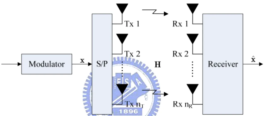
Figure 2.1: Block diagram of a spatial multiplexing system with nT transmit antennas

and nR receive antennas... 6

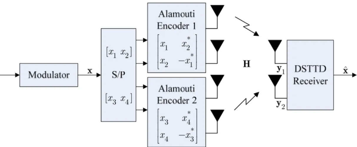
Figure 2.2: Block diagram of an Alamouti space-time coded system for two transmit antennas and single receive antenna ... 9 Figure 2.3: Block diagram of a DSTTD system with four transmit antennas and two

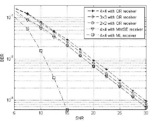
receive antennas ... 11 Figure 2.4: Average BER performances of spatial multiplexing MIMO systems with

different receivers with QPSK modulation ... 21 Figure 2.5: Average BER performances of DSTTD systems with different receivers

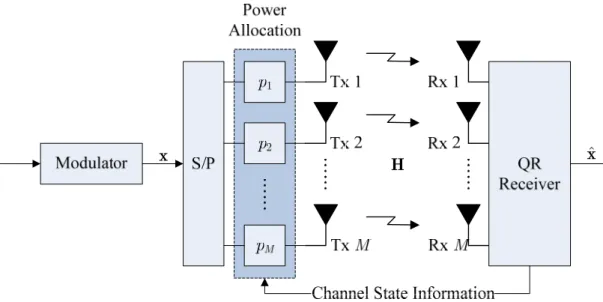
with QPSK modulation ... 21 Figure 3.1: Block diagram of a 4 spatial multiplexing MIMO system with the QR

receiver with the transmit power allocation scheme ... 25

4 ×

Figure 3.2: Evaluations of upper bounds for the lower bound of overall average BER in spatial multiplexing systems with the QR receiver with QPSK

modulation... 34

4 4×

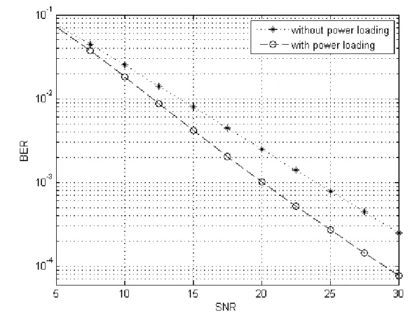
Figure 3.3: Average BER performances of spatial multiplexing systems with different receivers with QPSK modulation ... 35

4 4×

Figure 3.4: Average BER performances of spatial multiplexing systems with the QR receivers with different modulation orders... 35

4 4×

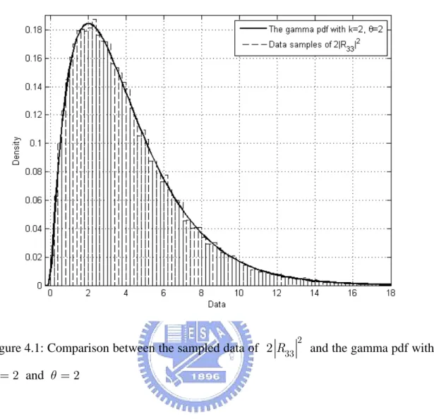
Figure 4.1: Comparison between the sampled data of 2 R₃₃2 and the gamma pdf with and ... 42

2

k = θ =2

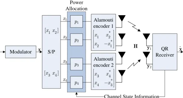
Figure 4.2: Block diagram of a DSTTD system with the QR receiver with transmit power allocation scheme ... 44 Figure 4.3: Comparisons between 2 R₃₃2, 2 R₅₅2 and the gamma pdfs with k =4,

2

θ = , and k =2, θ =2, respectively ... 49 Figure 4.4: Evaluations of upper bounds for the lower bound of average overall BER in

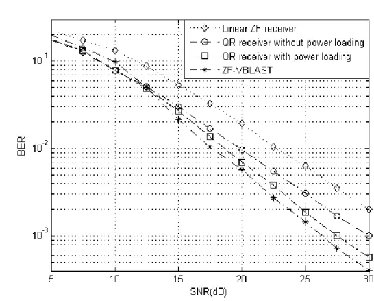
DSTTD systems with QPSK modulation... 52 Figure 4.5: Average BER performances of DSTTD systems with different receivers

with QPSK modulation ... 52 Figure 4.6: Average BER performances of DSTTD systems with the QR receiver with

different modulation orders... 53 Figure 4.7: Average BER performances of triple STTD systems with the QR receiver 53

Acronym Glossary

AWGN additive white Gaussian noise BER bit error rate

BLAST Bell laboratories layered space-time BPSK binary phase shift keying

BS base station

CIR channel impulse response CSI channel state information DSTTD double space-time transmit diversity EP error propagation

EQ equalizer

IEEE institute of electrical and electronics engineers ISI intersymbol interference

LB lower bound LOS line of sight

MIMO multiple-input multiple-output MISO multiple-input single-output ML maximum likelihood MMSE minimum mean-square error MRC maximal ratio combining MS mobile station

OSTBC orthogonal space-time block code PL power loading

QAM quadrature amplitude modulation QPSK quadrature phase shift keying SDMA spatial division multiple access SIMO single-input multiple-output SISO single-input single-output SM spatial multiplexing SNR signal-to-noise ratio

SIC successive interference cancellation STBC space-time block code

STTD space-time transmit diversity

V-BLAST vertical Bell laboratories layered space-time

Notations

s

E symbol energy T

n number of transmit antennas R

n number of receive antennas

0

N noise power spectrum density

R rate of space-time codes

P power loading matrix ρ instantaneous SNR

M number of transmission links

Chapter 1

Introduction

Multiple-input multiple-output (MIMO) systems, employing several transmit and receive antennas at both ends, are capable of providing a significant increase in capacity compared to traditional single-input single-output (SISO) systems [1], [2]. The spatial multiplexing technique was proposed to increase system capacity. On the other hand, orthogonal space-time code designs [3], [4] generally yield good bit error rate (BER) performance. Space-time transmit diversity (STTD) as well as Alamouti space-time block codes (STBCs) was introduced to provide transmit diversity gain. One main limitation of these schemes providing transmit diversity is that they do not achieve full rate, which, for a single channel, means that each transmitter antenna transmits one symbol per second per Hertz. To exploit these two advantages at the same time, double space-time transmit diversity (DSTTD) with four antennas was suggested in [5], [6]. In this system, two STTD encoders are used at the transmitter and interference cancellation based detector is employed at the receiver.

When the transmitter has acquired some knowledge of the channel state information (CSI), a precoder can be applied at the transmitter to improve the performance of the system. With full knowledge of CSI, a minimum mean-square error (MMSE) precoder has been designed in [8]. To reduce the requirement of CSI feedback,

Space-Time (V-BLAST) detection [16]. The design adjusts the power and rate of each antenna to minimize either the maximum BER of all sub-streams or the total transmission power. However, when the transmission rates in the antennas are equal, this may lead to the result of equal power allocation.

This thesis addresses the symbol detection problem of spatial multiplexing MIMO systems and DSTTD systems over i.i.d. Rayleigh fading channels. To achieve the BER performance balance between linear receivers and joint maximum likelihood (ML) detection, a QR-based successive symbol detection scheme with proper symbol power allocation is proposed. There have been many performance measures for successive symbol recovery in spatial multiplexing systems and DSTTD systems discussed in [9]-[15]. The average BER with error free front-layer decision feedback, though just a lower bound of the exact mean error rate, is simple to characterize and, furthermore, is closely related to the upper bound of the block error rate when error propagation occurs [15]. Thus, it becomes an efficient and meaningful performance metric accounting for the actual BER performance analysis. Motivated by this fact and to also guarantee the performance improvements regardless of the instantaneous channel conditions, a power allocation scheme aiming to minimizing the overall BER averaged with respect to the channel distribution is proposed. Specific contributions of this thesis include:

1. By exploiting the distinctive channel matrix structure induced by DSTTD, we derive an explicit formula for the associated QR decomposition.

2. With the approved statistical property of the R matrix in QR decomposition for spatial multiplexing systems and DSTTD systems, the closed-form upper bounds for the BER metric are obtained.

3. By minimizing the upper bounds, an optimal power allocation scheme is proposed, and is obtained through numerical search.

has been addressed in many previous researches [9]-[16], all of them are based on a given fixed channel realization known to the transmitter. The strategy proposed in this thesis is grounded on the overall BER averaged over the channel distribution; that is, it is independent of the instantaneous channel condition, and thus requires fewer feedback messages from the receiver. Furthermore, the distribution of QR decomposition for DSTTD is discovered. This makes it possible to apply the design criterion to DSTTD systems, and even multiple STTD systems.

This thesis is organized as follows. In Chapter 2, the review of spatial multiplexing MIMO systems and DSTTD systems is introduced, and the statistical property and particular matrix structure of QR decompositions for spatial multiplexing and DSTTD are stated. Additionally, the system models of spatial multiplexing and DSTTD with QR-based successive detection are also built. In Chapter 3, with knowledge of distribution of the R matrix for spatial multiplexing, a power allocation scheme which aims to minimize the overall average BER performance of spatial multiplexing systems is proposed. In Chapter 4, the probability density functions (pdfs) of the matrix for DSTTD systems are calculated and estimated. With the exact and approximated pdfs, the power loading factors proposed for DSTTD systems are obtained. Computer simulations of BER performances of the proposed scheme are then illustrated. Finally, we conclude this thesis and describe some potential future works in Chapter 5.

Chapter 2

Model of MIMO Wireless

Communication Systems

Equation Section 2

This chapter first presents the review of spatial multiplexing (SM) and double space-time transmit diversity (DSTTD). Spatial multiplexing scheme is a promising technique to enhance data rate, and it can only be implemented in multiple-input multiple-output (MIMO) systems. Before the review of DSTTD systems, we will give an introduction to Alamouti space-time transmit diversity. DSTTD system is basically a simple combination of spatial multiplexing and space-time transmit diversity such that both capacity and reliability can be achieved simultaneously. Afterwards, we will review the QR decomposition and introduce the QR decompositions of spatial multiplexing systems and DSTTD systems. We detect the received symbols by exploiting these special structures and compare their performances with the conventional detection methods.

2.1

Review of Spatial Multiplexing

Spatial multiplexing is capable of offering a linear increase in the transmission rate (or capacity) for the same bandwidth and without additional power consumption. The

minimum of number of transmit antennas and that of receive antennas. The bit stream to be transmitted is divided into multiple sub-streams, modulated and transmitted simultaneously from each transmit antenna [1]. Under favorable channel conditions, the spatial signatures of these signals induced at the receive antennas can be well separated. The receiver, having knowledge of the channels, is able to differentiate among the co-channel signals and extract all signals, after which demodulation yields the original sub-streams that can now be combined to give the original bit stream. Spatial multiplexing can also be applied in a multi-user format (MIMO-MU, also known as space division multiple access or SDMA).

We assume that in spatial multiplexing MIMO systems there are transmit antennas at transmitter and receive antennas at receiver. The channel response from transmit antenna to receive antenna i , , is assumed flat and can be modeled as an i.i.d. complex zero-mean Gaussian variable with unit variance. Let be the symbol to be transmitted from antenna , and the received signal on receive antenna , T n R n j h_ij i x i j y_j, is given by 1 1 2 2 _{T T}. j j j n j y =h x +h x + +h x_n (2.1)

Accordingly, we can express the spatial multiplexing MIMO systems in matrix form:

11 12 1 1 1 1 2 21 22 2 2 2 1 2 , T T R _{R R R T} T R n n n _{n n n n} n n h h h y x n y h h h x n y h h h x n ⎡ ⎤ ⎡ ⎤ _{⎢ ⎥}⎡ ⎤ ⎡ ⎤ ⎢ ⎥ _{⎢ ⎥}⎢ ⎥ ⎢ ⎥ ⎢ ⎥ _{⎢ ⎥}⎢ ⎥ ⎢ ⎥ ⎢ ⎥ ⎢ ⎥ ⎢ ⎥ =⎢ ⎥ = ⎢_⎢ ⎥_⎥⎢ ⎥+⎢ ⎥ = + ⎢ ⎥ _{⎢ ⎥}⎢ ⎥ ⎢ ⎥ ⎢ ⎥ _{⎢ ⎥}⎢ ⎥ ⎢ ⎥ ⎢ ⎥ _{⎢ ⎥ ⎣}⎢ ⎥_⎦ ⎢ ⎥ ⎣ ⎦ _{⎣ ⎦} ⎣ y H ⎦ x n ) R (2.2)

where are i.i.d. complex Gaussian random variables with zero mean and variance 1.

=1, ( 2, ..., i

n i n

is demultiplexed into sub-streams which are transmitted simultaneously. At receiver, the received data stream is obtained by combining the detected received signals. Although spatial multiplexing technique is capable of providing a boost in transmission data rate, it can not induce diversity gain to improve the reliability of wireless communication systems. Therefore, we will discuss transmit diversity technique in the next section and give a simple transmission scheme to enhance the reliability of wireless communication systems.

T

n

x ˆx

H

Figure 2.1: Block diagram of a spatial multiplexing system with nT transmit antennas

and nR receive antennas

2.2

Review of Double Space-Time Transmit

Diversity

Recently space-time transmit diversity (STTD) has been studied extensively as a method of combating detrimental effects in wireless fading channels because of its relative simplicity of implementation and feasibility of having multiple antennas at the base station. The first bandwidth efficient transmit diversity scheme was proposed by Wittneben [17], and it includes the delay diversity scheme of Seshadri and Winters [18] as a special case. More recently, space-time trellis coding has been proposed [3] which

combines signal processing at the receiver with coding techniques appropriate to multiple transmit antennas and provides significant gain over [17] and [18]. In addressing the issue of decoding complexity, Alamouti discovered a remarkable transmission scheme which can provide full rate and full diversity gain with two transmit antennas [4].

2.2.1 Alamouti Space-Time Transmit Diversity

In the Alamouti space-time transmit diversity scheme, we consider two antennas at the transmitter and a single receive antenna. Assume that an M-ary modulation is used and each group of m information bits is modulated, where . The symbols to be space-time encoded are divided into groups of two symbols in each encoding operation. Two different symbols and in each group are transmitted simultaneously from antennas 1 and 2 respectively during the first symbol period. During the next symbol period, is transmitted form antenna 1 and is transmitted from antenna 2. Superscripts ( ) , , and ( ) denote transpose, complex conjugate, and Hermitian operation, respectively.

2 log m = M ⎤⎥⎦ 1 x x₂ * 2 x −x₁* T i ( )i* i H

We assume that the channel remains constant over the two symbol periods, and is frequency flat. Let and be the fading channel coefficients from antenna 1 and antenna 2. The real part and imaginary part of channel coefficients are modeled as Gaussian random variables with zero mean and variance 0.5. Consequently,

and the signals and received over the two symbol periods are given by 1 h h₂ 1 2 T h h ⎡ = ⎢⎣ h y₁ y₂

(2.3) 1 1 1 2 2 , y =h x +h x +n₁ 2 (2.4) * * 2 1 2 2 1 , y =h x −h x +n

where and are i.i.d. complex Gaussian random variables with zero mean. The real part and imaginary part of noise have the same variance

1

n n₂

(2 )

T

n SNR , where SNR stands for the average signal-to-noise ratio. The received signals can be written as

1 2 1 1 * * 2 2 1 2 , x x y h y x x h 1 2 n n ⎡ ⎤ ⎡ ⎤ _{⎢ ⎥}⎡ ⎤ ⎡ ⎤ ⎢ ⎥ _{= ⎢ ⎥}⎢ ⎥ ⎢ ⎥ ⎢ ⎥ _{⎢ − ⎥}⎢ ⎥ ⎢ ⎥ ⎢ ⎥ ⎢ ⎥ ⎢ ⎥ ⎣ ⎦ ⎣ ⎦ ⎣ ⎦ + ⎣ ⎦ (2.5)

and we can obtain a rearranged signal vector y as follows:

1 1 2 1 1 * * * * 2 2 2 1 2 . y h h x n x y h h n ⎡ ⎤ ⎡ ⎤⎡ ⎤ ⎡ ⎤ ⎢ ⎥ ⎢ ⎥⎢ ⎥ ⎢ ⎥ =_{⎢ ⎥} =_{⎢ ⎥⎢ ⎥}+_{⎢ ⎥} = + − ⎢ ⎥ ⎢ ⎥⎢ ⎥_{⎣ ⎦} ⎢ ⎥ ⎣ ⎦ ⎣ ⎦ ⎣ ⎦ y Hx n (2.6)

The channel matrix H is orthogonal (i.e., H 2 ₂ F = H H h I ). If , we can get H = z H y 2 2 , H H F = + = + z H Hx H n h I x n (2.7) where { } _2,1 and { H} 2 _{0 2} F

E n =0 E nn = h N I . Hence, the effective channel for symbols x i_i ( =1, 2) becomes 1, 2, 2 , i _F i i z = h x +n i = (2.8)

and the receive SNR, η, per symbol is given by

2

, 2

F ρ

η = h (2.9)

where ρ E N_{s 0} is the average signal-to-noise ratio (SNR).

The block diagram that includes modulator, serial to parallel structure and Alamouti space-time encoder is shown in Figure 2.2. The data stream is demultiplexed

into two sub-streams which are converted from serial to parallel and mapped to an Alamouti encoder. The Alamouti scheme extracts a diversity order of 2 (full diversity), even in the absence of channel knowledge at the transmitter.

T n x [x x1 2] * 1 2 * 2 1 x x x x ⎡ ⎤ ⎢ ⎥ ⎢ ⎥ ⎢ − ⎥ ⎣ ⎦ 1 h 2 h y ˆx

Figure 2.2: Block diagram of an Alamouti space-time coded system for two transmit antennas and single receive antenna

2.2.2 Double Space-Time Transmit Diversity Systems

After the review of Alamouti space-time transmit diversity, combining spatial multiplexing technique with it, we then introduce the concept of double space-time transmit diversity (DSTTD) systems. The DSTTD system is an open-loop multiple-input multiple-output system with four transmit antennas and two receive antennas. It has two Alamouti space-time encoders at transmitter and obtains high data rate as well as transmit diversity.

In DSTTD system, four symbols are transmitted during two symbol periods. The symbols are first arranged into two groups and , and they are then mapped into two Alamouti space-time encoders respectively. Let be the channel coefficient from transmit antenna to receive antenna , and it is complex Gaussian with zero mean and unit variance. At receiver

1 2 3 4 { ,x x , x , x } 1 2 { ,x x } 3 4 { ,x x } ij h j i

antenna 1, the received signals during two symbol periods can therefore be written in matrix form as

1,1 1,2 [y y ]T n n 11 1 2 3 4 1,1 12 1,1 * * * * 1,2 2 1 4 3 13 1,2 14 , h x x x x y h y x x x x h h ⎡ ⎤ ⎢ ⎥ ⎡ ⎤ ⎢ ⎥ ⎡ ⎤ _{⎢ ⎥ ⎢ ⎥} ⎡ ⎤ ⎢ ⎥ _{= ⎢ ⎥ ⎢} ⎢ ⎥ ⎥ ⎢ ⎥ _{⎢ − − ⎥ ⎢ ⎥} ⎢ ⎥ ⎢ ⎥ ⎢ ⎥ ⎣ ⎦ ⎣ _{⎦ ⎢ ⎥} ⎣ ⎦ ⎢ ⎥ + ⎣ ⎦ (2.10)

where is noise on receive antenna i at symbol period t , which is assumed complex zero-mean Gaussian with variance 1. We can express with similar formulation: , i t n 2,1 2,2 [y y ]T n n 21 1 2 3 4 2,1 22 2,1 * * * * 2,2 2 1 4 3 23 2,2 24 . h x x x x y h y x x x x h h ⎡ ⎤ ⎢ ⎥ ⎡ ⎤ ⎢ ⎥ ⎡ ⎤ _{⎢ ⎥ ⎢ ⎥} ⎡ ⎤ ⎢ ⎥ _{= ⎢ ⎥ ⎢ ⎥} ⎢ ⎥ ⎢ ⎥ _{⎢ − − ⎥ ⎢ ⎥} ⎢ ⎥ ⎢ ⎥ ⎢ ⎥ ⎣ ⎦ ⎣ _{⎦ ⎢ ⎥} ⎣ ⎦ ⎢ ⎥ + ⎣ ⎦ (2.11)

Combining (2.10) and (2.11), we can rearrange the received signals as follows:

1,1 11 12 13 14 ₁ 1,1 * * * * * * 1 1,2 12 11 14 13 2 1,2 2 2,1 21 22 23 24 3 2,1 * * * * * * 4 2,2 22 21 24 23 2,2 y h h h h _x n y h h h h x n y h h h h x n x y h h h h n ⎡ ⎤ ⎡ ⎤_{⎡ ⎤} ⎡ ⎤ ⎢ ⎥ ⎢ ⎥_{⎢ ⎥} ⎢ ⎥ ⎢ ⎥ ⎢ ⎥_{⎢ ⎥} ⎢ ⎥ ⎡ ⎤ _{⎢ ⎥ ⎢− − ⎥⎢ ⎥ ⎢ ⎥} ⎢ ⎥ =_{⎢ ⎥} =⎢ ⎥ =⎢ ⎥_{⎢ ⎥}+⎢ ⎥ ⎢ ⎥ ⎢ ⎥_{⎢ ⎥} ⎢ ⎥ ⎢ ⎥ ⎣ ⎦ _{⎢ ⎥ ⎢ ⎥⎢ ⎥ ⎢ ⎥} ⎢ ⎥ ⎢_{− −} ⎥_{⎢ ⎥⎣ ⎦} ⎢ ⎥ ⎢ ⎥ ⎢ ⎥ ⎢ ⎣ ⎦ ⎣ ⎦ ⎣ ⎦ y y y = + . ⎥ Hx n (2.12)

The block diagram of a DSTTD system with four transmit antennas and two receive antennas is shown in Figure 2.3. The data stream is demultiplexed into four sub-streams which are divided into two groups. Each group of two sub-streams is encoded by an Alamouti space-time encoder.

1 y 2 y H x 1 2 [x x ] 3 4 [x x ] * 1 2 * 2 1 x x x x ⎡ ⎤ ⎢ ⎥ ⎢ ⎥ ⎢ − ⎥ ⎣ ⎦ * 3 4 * 4 3 x x x x ⎡ ⎤ ⎢ ⎥ ⎢ ⎥ ⎢ − ⎥ ⎣ ⎦ ˆx

Figure 2.3: Block diagram of a DSTTD system with four transmit antennas and two receive antennas

2.3 QR

Decomposition

of

Channel

Matrix

In this section, we will introduce the QR decompositions of spatial multiplexing MIMO systems and double space-time transmit diversity systems. The diagonal entries of for spatial multiplexing systems are related to chi-square distribution, and this let us be able to find a performance bound of spatial multiplexing systems. For QR decomposition of DSTTD systems has a special structure, and the diagonal entries of it are found to be associated with the entries of the DSTTD channel matrix.

R

R

2.3.1 Review of QR Decomposition

QR decomposition is one of the well-known decompositions, and can be obtained by the Gram-Schmidt process straightforwardly. We know that the formulation of Gram-Schmidt procedure is to find an orthonormal basis for the space spanned by the original linearly independent basis. The Gram-Schmidt process frequently appears in the matrix form, and it is equivalent to QR decomposition. Let us show the lemma of QR decomposition and apply it to spatial multiplexing MIMO systems and double

space-time transmit diversity systems.

Lemma 2.1: Every matrix with linearly independent columns can be uniquely factored as in which the columns of are an orthonormal basis for

and is an upper triangular matrix with positive diagonal entries. m n× H = H QR Q_{m n×} ( ) R H R_{m n×}

Based on Lemma 2.1, we are going to apply QR decomposition to spatial multiplexing MIMO systems and DSTTD systems respectively in the next two sections.

2.3.2 QR Decomposition of Channel Matrix in Spatial

Multiplexing MIMO Systems

In spatial multiplexing MIMO systems, the channel matrix is defined as a standard complex Gaussian matrix which has i.i.d. complex zero-mean Gaussian entries with identical variance 1. Though the QR decomposition of i.i.d. MIMO channel matrix has no special structure, there is still a lemma in random matrix theory worth mentioning. R n ×n_T ii R i∈ m j H

Lemma 2.2: Let be an m standard complex Gaussian matrix with . Denote its QR decomposition by . The upper triangular matrix is independent of Q. The entries of are independent and its diagonal entries, , are such that are chi-square random variables with degrees of freedom while the off-diagonal entries, , are independent zero-mean complex Gaussian with variance 1.

H ×n n ≥m = H QR R R for {1,..., } 2R_ii2 2(n− +i 1) R_ij for i <

We will discuss it later in Chapter 3.

2.3.3 QR Decomposition of Channel Matrix in Double

Space-Time Transmit Diversity Systems

First, the properties of Alamouti block are introduced. They are important in deriving the QR decomposition of DSTTD systems. We list some fundamental properties as follows:

1. The sum of two Alamouti matrices is also an Alamouti matrix. 2. The product of two Alamouti matrices is also an Alamouti matrix. 3. The inverse of an Alamouti matrix is also an Alamouti matrix.

It is easy to derive the above results and the proofs are omitted here. From the above properties, it is obvious that the Alamouti structure for block matrices is preserved if the matrix operation is performed. We arrange them and show Lemma 2.3 and Lemma 2.4 [19].

Lemma 2.3: For a square matrix constructed by Alamouti blocks, the inverse of is also constructed by Alamouti blocks. That is, it is a block matrix with Alamouti sub-blocks.

n n×

H

n n×

H

Here is a simple example to explain the above lemma. Consider a matrix with four Alamouti sub-blocks given by

4 4× H 1 2 4 4 3 4 , × ⎡ ⎤ ⎢ ⎥ = ⎢ ⎥ ⎢ ⎥ ⎣ ⎦ H H H H H (2.13)

and 11 12 13 14 * * * * 1 2 12 11 14 13 , , h h h h h h h h ⎡ ⎤ ⎡ ⎢ ⎥ ⎢ =_{⎢ ⎥} =_⎢ − − ⎢ ⎥ ⎢ ⎣ ⎦ ⎣ H H ⎤ ⎥ ⎥ ⎥⎦ . ⎤ ⎥ ⎥ ⎥⎦ × and (2.14) and 21 22 23 24 * * * * 3 4 22 21 24 23 , h h h h h h h h ⎡ ⎤ ⎡ ⎢ ⎥ ⎢ =_{⎢ ⎥} = _⎢ − − ⎢ ⎥ ⎢ ⎣ ⎦ ⎣ H H

Under some manipulations, it can be shown that all the sub-blocks in are also Alamouti block matrices by using the fundamental properties of Alamouti structure. By this example, we can know that the inverse of channel matrix in DSTTD systems has the same structure.

1 4 4 −

×

H

Lemma 2.4: For a square matrix which is constructed by Alamouti sub-blocks, assume is factored as , where the columns of are an orthonormal basis and is a square unitary matrix. is an upper triangular matrix with positive diagonal entries. Then, is also constructed by Alamouti sub-blocks. has a special structure which is a block matrix with multiples of along its diagonal and with Alamouti sub-blocks in its upper triangular part. Continue with the previous example

n n× H n n× H H_{n n×} =Q_{n n×} R_{n n} Q_{n n×} n n× Q R_{n n×} n n× Q n n× R 2 I 11 12 13 14 * * * * 12 11 14 13 21 22 23 24 * * * * 22 21 24 23 . h h h h h h h h h h h h h h h h ⎡ ⎤ ⎢ ⎥ ⎢_{− −} ⎥ ⎢ ⎥ = ⎢ ⎥ ⎢ ⎥ ⎢ ⎥ ⎢_{− −} ⎥ ⎢ ⎥ ⎣ ⎦ H (2.15)

and 11 12 13 14 11 13 14 * * * * * * 12 11 14 13 22 14 13 21 22 23 24 33 * * * * 44 22 21 24 23 0 0 , , 0 0 0 0 0 0 q q q q R R q q q q R R R q q q q R R q q q q R ⎡ ⎤ ⎡ ⎤ ⎢ ⎥ ⎢ ⎥ ⎢_{− −} ⎥ ⎢ ₋ ⎥ ⎢ ⎥ ⎢ ⎥ = ⎢_⎢ ⎥_⎥ =⎢ ⎥ ⎢ ⎥ ⎢ ⎥ ⎢ ⎥ ⎢− − ⎥ ⎢ ⎥ ⎢ ⎥ ⎣ ⎦ ⎣ ⎦ Q R (2.16)

where all 2 2× sub-blocks are all Alamouti block matrices.

The proof is given in Appendix A. From the proof we can discover that the and for diagonal entries of , and they can be written in terms of determinants of channel matrix and its partitioned matrices (Alamouti sub-blocks). Finally, we can arrange the above derivations and conclude this section with the following properties:

11 22

R =R R₃₃ =R₄₄ R

H

1. The channel matrix of DSTTD systems is given by

11 12 13 14 * * * * 1 2 12 11 14 13 3 4 21 22 23 24 * * * * 22 21 24 23 . h h h h h h h h h h h h h h h h ⎡ ⎤ ⎢ ⎥ ⎢ ⎥ ⎡ ⎤ _{⎢− − ⎥} ⎢ ⎥ =_{⎢ ⎥} = ⎢ ⎥ ⎢ ⎥ ⎢ ⎥ ⎣ ⎦ _{⎢ ⎥} ⎢_{− −} ⎥ ⎢ ⎥ ⎣ ⎦ H H H H H (2.17) It can be factorized as 11 12 13 14 11 13 14 * * * * * * 12 11 14 13 22 14 13 21 22 23 24 33 * * * * 44 22 21 24 23 0 0 . 0 0 0 0 0 0 q q q q R R q q q q R R R q q q q R R q q q q ⎡ ⎤⎡ _R ⎤ ⎢ ⎥ ⎢ ⎥ ⎢_{− −} ⎥ ⎢ ₋ ⎥ ⎢ ⎥ ⎢ ⎥ = = ⎢ _{⎥ ⎢ ⎥} ⎢ ⎥ ⎢ ⎥ ⎢ ⎥ ⎢ ⎥ ⎢− − ⎥ ⎢ ⎥ ⎢ ⎥ ⎣ ⎦ ⎣ ⎦ H QR (2.18)

2. The diagonal entries of R can be expressed as

11 22 det( 1) det( 3), R =R = H + H (2.19) and 33 44 1 3 det( ) , det( ) det( ) R =R = + H H H (2.20)

2 2 2 1 11 12 2 13 14 det(H )= h + h , det(H )= h + h 2, and 2 2 2 3 21 22 4 23 24 det(H )= h + h , det(H )= h + h 2. (2.21)

2.4 Model

of

MIMO

Wireless

Communication

Systems with QR-Based Successive Detection

From the above discussions, in this section we will introduce the models of the two wireless communication systems. The symbol detection of QR-based receiver is based on unordered successive interference cancellation (SIC). In spatial multiplexing MIMO systems, symbol detection in one stage depends on the decisions made in the previous stages. Detection in DSTTD systems experiences the same effect, but in a group-wise manner; that is, symbols encoded by the same Alamouti space-time encoder will not interfere with each other.

2.4.1 Model of Spatial Multiplexing MIMO systems

We consider a spatial multiplexing MIMO systems whose channel matrix is given by 4 4× 11 12 13 14 21 22 23 24 31 32 33 34 41 42 43 44 , h h h h h h h h h h h h h h h h ⎡ ⎤ ⎢ ⎥ ⎢ ⎥ ⎢ ⎥ = ⎢ ⎥ ⎢ ⎥ ⎢ ⎥ ⎢ ⎥ ⎣ ⎦ H (2.22)

which can be factorized as

(2.23) 11 12 13 14 11 12 13 14 21 22 23 24 22 23 24 31 32 33 34 33 34 41 42 43 44 44 0 . 0 0 0 0 0 q q q q R R R R q q q q R R R q q q q R R q q q q R ⎡ ⎤ ⎡ ⎢ ⎥ ⎢ ⎢ ⎥ ⎢ ⎢ ⎥ ⎢ = _{= ⎢ ⎥ ⎢} ⎢ ⎥ ⎢ ⎢ ⎥ ⎢ ⎢ ⎥ ⎢ ⎣ ⎦ ⎣ H QR ⎤ ⎥ ⎥ ⎥ ⎥ ⎥ ⎥ ⎥⎦

Since is upper triangular, successive symbol detection through canceling the contributions of the previously detected components can be performed, as in

R

[15], [16]. From Equations (2.2) and (2.23), the received signals are multiplied by the unitary matrix QH to yield (2.24) 1 11 12 13 14 1 1 2 22 23 24 2 2 3 33 34 3 3 4 44 4 4 0 , 0 0 0 0 0 y R R R R x n y R R R x n y R R x n y R x n ⎡ ⎤ ⎡ ⎤ ⎡ ⎤ ⎡ ⎤ ⎢ ⎥ ⎢ ⎥ ⎢ ⎥ ⎢ ⎥ ⎢ ⎥ ⎢ ⎥ ⎢ ⎥ ⎢ ⎥ ⎢ ⎥ ⎢ ⎥ ⎢ ⎥ ⎢ ⎥ = _{⎢ ⎥} = _{⎢ ⎥ ⎢ ⎥}+_{⎢ ⎥} = + ⎢ ⎥ ⎢ ⎥ ⎢ ⎥ ⎢ ⎥ ⎢ ⎥ ⎢ ⎥ ⎢ ⎥ ⎢ ⎥ ⎢ ⎥ ⎢ ⎥ ⎢ ⎥ ⎢ ⎥ ⎣ ⎦ ⎣ ⎦ ⎣ ⎦ ⎣ ⎦ y Rx n j i y R = + = −

_∑

4,

where and . It is noted that and have an identical distribution since is unitary. Equation (2.24) can be expressed as follows:

H = y Q y n =Q nH n n H Q (2.25) 4 1 , 1, 2, 3, 4. i ii i ij j i j i y R x R x n i = + = +

_∑

+ =

Then we can get the modified received signals

(2.26) ˆ_i y 4 1 ˆ i ij jx 4 1 ˆ ( ) , 1, 2, 3, ii i ij j j i j i R x R x x n i = + = +

_∑

− + =

where xˆ_j is the symbols detected in the previous detection stages. Therefore, to detect symbol x_i, we will need to know the detected symbols xˆ_j (j = +i 1, i +2, ..., 4). The detection procedure can be described by the following expressions:

for . 4 1 ˆ ˆ_i Quant i j i ij j 1, 2, 3, 4 ii y R x x R = + ⎡ ₋ ⎤ ⎢ ⎥ = ⎢ ⎥ ⎢ ⎥ ⎢ ⎥ ⎣ ⎦

∑

i = b (2.27)

The function sets a to the element of signal constellations that is closet to . Assuming that these decisions are correct (

Quant a = ⎡ ⎤_{⎢ ⎥⎣ ⎦}

b x_j =xˆ_j), Equation (2.26) is

2.4.2 Model of Double Space-Time Transmit Diversity

Systems

In DSTTD systems, for its special channel matrix structure, the symbols grouped together will not affect each other. The channel matrix is given by

11 12 13 14 * * * * 12 11 14 13 21 22 23 24 * * * * 22 21 24 23 , h h h h h h h h h h h h h h h h ⎡ ⎤ ⎢ ⎥ ⎢_{− −} ⎥ ⎢ ⎥ = ⎢ ⎥ ⎢ ⎥ ⎢ ⎥ ⎢_{− −} ⎥ ⎢ ⎥ ⎣ ⎦ H (2.28)

and its QR decomposition is obtained as follows:

and 11 12 13 14 11 13 14 * * * * * * 12 11 14 13 11 14 13 21 22 23 24 33 * * * * 33 22 21 24 23 0 0 , . 0 0 0 0 0 0 q q q q R R q q q q R R R q q q q R R q q q q R ⎡ ⎤ ⎡ ⎤ ⎢ ⎥ ⎢ ⎥ ⎢_{− −} ⎥ ⎢ ₋ ⎥ ⎢ ⎥ ⎢ ⎥ = ⎢_⎢ ⎥_⎥ = ⎢ ⎥ ⎢ ⎥ ⎢ ⎥ ⎢ ⎥ ⎢− − ⎥ ⎢ ⎥ ⎢ ⎥ ⎣ ⎦ ⎣ ⎦ Q R (2.29)

Similar to the expressions in the previous section, from Equations (2.12) and (2.29), the received signals can be written as

(2.30) 11 13 14 1 1 * * 2 11 14 13 2 3 33 3 4 33 4 0 0 , 0 0 0 0 0 0 R R R y x y R R R x y R x y R x ⎡ ⎤ ⎡ ⎤ _{⎢ ⎥}⎡ ⎤ ⎡ ⎤ ⎢ ⎥ _{⎢ ⎥}⎢ ⎥ ⎢ ⎥ ⎢ ⎥ _{⎢ − ⎥}⎢ ⎥ ⎢ ⎥ ⎢ ⎥ ⎢ ⎥ ⎢ ⎥ = _{⎢ ⎥} = _{⎢ ⎥⎢ ⎥}+_{⎢ ⎥}= + ⎢ ⎥ ⎢ ⎥ _{⎢ ⎥}⎢ ⎥ ⎢ ⎥ ⎢ ⎥ _{⎢ ⎥}⎢ ⎥ ⎢ ⎥ ⎢ ⎥ ⎢ ⎥ ⎢ ⎥ ⎣ ⎦ ⎣ ⎦⎣ ⎦ ⎣ ⎦ y R 1 2 3 4 n n n n x n 4

and this equation is equivalent to

(2.31) 1 11 1 13 3 14 * * 2 11 2 14 13 4 3 33 3 4 33 4 , , , . x y R x R x R x y R x R x R x y R x y R x = + + = − + = =

Thus, the detection procedure can be described by the following formulas:

4 4 33 ˆ Quant y , x R ⎡ ⎤ ⎢ ⎥ = _{⎢ ⎥} ⎢ ⎥ ⎣ ⎦ 3 3 33 ˆ Quant y , x R ⎡ ⎤ ⎢ ⎥ = _{⎢ ⎥} ⎢ ⎥ ⎣ ⎦

* * 2 14 3 13 4 2 11 ˆ Quant y R x R x , x R ⎡ _{+ −} ⎤ ⎢ ⎥ = _{⎢ ⎥} ⎢ ⎥ ⎣ ⎦ and ₁ 1 13 3 14 4 11 ˆ Quant y R x R x . x R ⎡ _{+ −} ⎤ ⎢ ⎥ = _{⎢ ⎥} ⎢ ⎥ ⎣ ⎦ (2.32)

As we can see in Equation (2.32), and can be detected individually, and then and can be decided with the decisions made for and . The simulations are provided and compared with the MMSE detector.

3

x x₄

1

x x₂ x₃ x₄

2.5 Computer

Simulations

In the simulation results, we first examine the performances of spatial multiplexing MIMO systems. Assume that QPSK modulation is adopted and the fading channels are flat. The channel coefficients are i.i.d. complex Gaussian random variables with zero mean and unit variance. The noise is complex zero-mean Gaussian random variable with unit variance. In Figure 2.4, the performances of spatial multiplexing MIMO systems with different numbers of transmit-receive antenna pairs and with different detection schemes are presented. As we can see in Figure 2.4, in spatial multiplexing systems with ML detection at the receiver, ML receiver is capable of extracting four-order spatial diversity because the ML detecting process outputs the most likely transmitted signal vector, so that the receiver spatial diversity can be fully obtained. The linear receivers like QR receiver and MMSE receiver can only extract one-order spatial diversity for all degrees of freedom of the transmission systems are exploited to increase the capacity. In spatial multiplexing systems, MMSE receiver performs better than QR receiver. Further, for QR receiver, when the number of parallel channels increases, the performances degrade slightly. One reason for this is

power sharing among the transmit antennas; since the normalization keeps the total transmit energy constant, in spatial multiplexing the power per stream is reduced by a factor of . Another reason is that when the number of data streams increases, in QR detection the average performances will become poorer due to cross-stage error propagation.

R

n

In DSTTD systems, the simulation results for different receivers are shown in Figure 2.5. The performances of DSTTD systems with QR receiver and MMSE receiver are quite comparable. That is, we can provide similar average BER performances with QR-based successive detection compared with the MMSE detection. Because of the transmit diversity provided by Alamouti space-time encoder, compared with the performance in spatial multiplexing for the same transmission rate, DSTTD systems have a two-order spatial diversity which is higher than unordered spatial multiplexing schemes. With ML receiver, a four-order spatial diversity can be achieved since ML receiver is able to extract the two-order receive spatial diversity in DSTTD systems.

Figure 2.4: Average BER performances of spatial multiplexing MIMO systems with different receivers with QPSK modulation

Figure 2.5: Average BER performances of DSTTD systems with different receivers with QPSK modulation

2.6 Summary

In wireless communication systems, spatial multiplexing techniques are widely used to exploit the characteristics of multipath channels and to improve the capacity of transmission without allocating extra bandwidth. On the aspect of diversity techniques, which is implemented to reduce the effects of multipath fading and to enhance the reliability of transmission without increasing the transmit power or sacrificing the bandwidth, it is popular to make use of space diversity which can be classified into two categories, transmit diversity and receive diversity. In this chapter, we focus on two high-rate wireless communication systems, simple spatial multiplexing and double space-time transmit diversity. Spatial multiplexing systems can provide a high date rate but no diversity gain can be obtained. Thus, a compromised transmission scheme, double space-time transmit diversity, is introduced. Compared to conventional SISO systems, DSTTD can provide a double rate and double diversity at the same time.

The QR decompositions of spatial multiplexing and DSTTD systems are characterized in Section 2.3. Based on the results of QR decomposition, the structures of the upper triangular matrix are shown in Equation (2.23) and (2.29). It is useful for us to detect the received signals and provide better performance. Furthermore, in DSTTD systems, we derive the diagonal entries of the upper triangular matrix and express them in terms of the determinants of the channel matrix and its partitioned matrices. Then, some performance comparisons are illustrated in Section 2.5. Since QR detector is an unordered SIC detector, its performance is slightly poorer than the performance of MMSE detector. In the next two chapters, we will exploit the precoding matrix to allocate the transmit power and reduce the average bit error rate (BER). That is, we focus on the power allocation scheme by using the statistical properties of with QR-based SIC detection in spatial multiplexing and DSTTD systems.

Chapter 3

Power Allocation for Minimum BER

in Spatial Multiplexing Systems

Equation Section 3

In this chapter, we will discuss the power allocation scheme with QR-based successive detection for spatial multiplexing MIMO systems over flat fading channels. Our consideration is confined to uncoded quadrature phase-shift keying (QPSK) signals and the channels are independent and identically distributed Rayleigh fading. Given that the channel state information (CSI) is perfectly available at the receiver and only signal-to-noise ratio (SNR) is known at the transmitter, we design a precoding matrix to allocate transmit power at the transmitter under average channel realizations. Furthermore, at the receiver, the received signals are detected with a QR-based successive symbol detecting scheme which is described in the previous chapter. For simplicity, the precoding matrix is restricted to be a diagonal power loading matrix so as to reduce the computational complexity. The optimization criterion is determined based on minimizing the overall average bit error rate (BER) of this transmission scheme. From the theory in [15], the design of the precoding matrix is based on the minimization of the lower bound for average BER. It can be proved that minimizing the lower bound for average BER will lead to minimizing the upper bound for the block error rate simultaneously. Following that, we exploit the power loading factors derived

from the closed-form solutions which we obtain by averaging the lower bound for BER over the channel realizations. Finally, some performance comparisons and discussions will be illustrated in the end of this chapter.

3.1

Bound for BER of QR-Based Successive

Detection

Power loading schemes allocate the transmit power across symbols under the constraint of constant power per block. At the transmitter, for four symbols

transmitted at the same time, we denote the transmit power allocated to the th symbol as and define the power loading matrix as

, 1, 2, 3, i x i = 4 0 i p_i2 1 2 3 4 0 0 0 0 0 , 0 0 0 0 0 0 p p p p ⎡ ⎤ ⎢ ⎥ ⎢ ⎥ ⎢ ⎥ = ⎢ ⎥ ⎢ ⎥ ⎢ ⎥ ⎢ ⎥ ⎣ ⎦ P (3.1)

where is the power loading factor ,and the block transmit power constraint must be normalized as 0 i p > (3.2) 4 2 1 trace{ H } _i 4. i p = =

_∑

= P P

Assuming that the channels are flat fading, we insert the power loading matrix into the system model in Equation (2.24). If the receiver replies the channel state information (CSI) to the transmitter, the transmitter can determine the power loading factors by the CSI. The block diagram with the transmit power allocation scheme is shown in Figure 3.1.

x ˆx

H

Figure 3.1: Block diagram of a spatial multiplexing MIMO system with the QR receiver with the transmit power allocation scheme

4 4×

The received signals are multiplied from the left by the unitary matrix from QR decomposition, and they can be written as

H Q 1 11 12 13 14 1 1 1 2 22 23 24 2 2 2 3 33 34 3 3 3 4 44 4 4 4 0 0 0 0 0 0 0 , 0 0 0 0 0 0 0 0 0 0 0 y R R R R p x n y R R R p x n y R R p x n y R p x n ⎡ ⎤ ⎡ ⎤ ⎡ ⎤ ⎡ ⎤ ⎡ ⎤ ⎢ ⎥ ⎢ ⎥ ⎢ ⎥ ⎢ ⎥ ⎢ ⎥ ⎢ ⎥ ⎢ ⎥ ⎢ ⎥ ⎢ ⎥ ⎢ ⎥ ⎢ ⎥ ⎢ ⎥ ⎢ ⎥ ⎢ ⎥ ⎢ ⎥ = _{⎢ ⎥} = _{⎢ ⎥ ⎢ ⎥ ⎢ ⎥}+_{⎢ ⎥}= + ⎢ ⎥ ⎢ ⎥ ⎢ ⎥ ⎢ ⎥ ⎢ ⎥ ⎢ ⎥ ⎢ ⎥ ⎢ ⎥ ⎢ ⎥ ⎢ ⎥ ⎢ ⎥ ⎢ ⎥ ⎢ ⎥ ⎢ ⎥ ⎢ ⎥ ⎣ ⎦ ⎣ ⎦ ⎣ ⎦ ⎣ ⎦ ⎣ ⎦ y RPx n j i y R = + = −

_∑

. i (3.3)

where and . The i th element of modified received signals is detected as follows: H = y Q y n=Q nH (3.4) ˆ_i y 4 1 ˆ i ij j jp x 4 1 ˆ ( ) ii i i ij j j j i j i R p x R p x x n = + = +

_∑

− +

Assume that there is no error in the previous symbol detection, and then we can obtain . It is obvious that the i th modified received signal is determined by the th transmitted symbol and the transformed channel noise. As long as the symbol in each stage is correctly detected and, hence, there is no layer-wise error

ˆ_{i ii i i}

y =R p x +n i

The power loading factor represents the transmit power allocated to the i th sub-channel and is the i th sub-channel gain. The average energy of the symbols transmitted from each antenna is normalized to be one. Therefore, the total symbol energy is equal to , so that the average power of received signal at each receive antenna is also . The real part and imaginary part of noise have the same variance 2 i p ii R s E n_T T n (2 ) T

n SNR . The average signal-to-noise ratio (SNR) is defined by

0

s

E N

ρ , where the total symbol energy and noise variance are defined as and , respectively. At some ρ , the instantaneous BER under the th sub-channel is given by

4 { } 4 T H s n E xx =E I = I E{nnH}=N_{0 4}I i ( ei i ii P =Q ρ p R ), (3.5) where 2 ₂ 1 ( ) 2 y Q x _π e π ∞ −

∫

dy and QPSK modulation is adopted. Thus, the average

instantaneous BER of the symbol block given a fixed channel realization is expressed as 4 4 1 1 1 1 ( 4 4 e ei i i i P P Q ρ p R = = =

_∑

=

_∑

_ii ). (3.6)

It is noted that the above discussion is under the error propagation free case; that is, error propagation is not taken into account. In this case, Equation (3.6) is merely a lower bound for average BER, and we rewrite it as

4 4 1 1 1 1 ( 4 4 eL eLi i ii i i P P Q ρ p = = =

_∑

=

_∑

R ), (3.7)

where the subscript indicates the lower bound for BER. This is a lower bound with QR-based successive symbol detection without considering the error propagation.

SNR regime because the error propagation is small enough to be neglected when SNR is high. If the error propagation occurs, the detection error of previous symbol decisions will affect the detection of the present symbol. This effect causes that the average BER with the error propagation is slightly higher than the average BER in the error propagation free case.

After the lower bound for average BER is presented, we will introduce the upper bound for average block error rate, which is of our major concern. First, let us define the detection error in the th symbol when there may be errors in the detection of previous symbols. We denote the received signal vector which would have been detected before by , and the transmitted signal vector which will be detected before by

i x_i

i

x xˆ_ei =[xˆ_i+1, ,xˆ ]₄T

i

x x_{ei = ⎢}⎡_⎣x_i+1, ,x₄⎤_⎥⎦T, respectively. For the detection of the th symbol i x_i, based on Bayes’ rule, we can get

ˆ { _{i i}} P x ≠x =P x{ _i ≠xˆ_i|x_ei =ˆx_ei}P{x_ei =xˆ_ei} +P x{ _i ≠xˆ_i |x_ei ≠ ˆx_ei}P{x_ei ≠ˆx }_ei . (3.8) } 1 1 } P x x = − = ˆ { _{i i}

P x ≠x |x_ei = ˆx_ei is equivalent to Equation (3.5) for the error propagation free case so that Equation (3.8) can be written as

ˆ { _{i i}} P x ≠x =P P_eLi {x_ei =ˆx_ei}+P x{ _i ≠xˆ_i|x_ei ≠xˆ_ei}P{x_ei ≠xˆ_ei} (3.9) ˆ { }. eLi ei ei P P ≤ + x ≠x

In the above equation, the last inequality is due to the fact that and for high SNR. Furthermore,

ˆ { _{i i} P x ≠x |x_ei ≠xˆ_ei}≤ P{x_ei =ˆx_ei}≅ ˆ { _{ei ei}} P x ≠ x = −1 P{x_ei =ˆx_ei 4 ˆ4 1 { }P x{ ₃ =xˆ₃|x₄ =xˆ₄} P x{ ₊ =xˆ₊ |x ₊ =ˆx ₊ }

(3.10) 4 4 1 1 1 _{j i= +} (1 P_eLj) _{j i= +} P_eLj. = −

_∏

− ≤

_∑

Because is written as

, the last equality is obtained which can be easily derived by some manipulations. Combining (3.9) and (3.10), the result is shown as

1 ˆ 1 { _{i i} P x ₊ =x ₊ |x_ei+1 =ˆx_ei+1} P ˆ 1−P x{ _i ≠x_i |x_ei = ˆx_ei) 1 P_eLj = − (3.11) ˆ { _{i i}} P x ≠x 4 4 1 ˆ { } , eLi ei ei

eLi eLj eLj eUi

j i j i P P P P P = + = ≤ + ≠ ≤ +

_∑

=

_∑

= x x

where the subscript indicates the upper bound for BER. Equation (3.11) represents the upper bound for the BER based on the consideration that there may be detection errors in the previous detected symbols. The upper bound for the average BER of four symbols is given by U 4 4 4 1 1 4 4 1 1 1 1 4 4 1 1 ( ) 4 4 eU eUi eLj i i j i eLi i ii i i P P P iP iQ ρ p R = = = = = = = = =

∑

∑ ∑

∑

∑

. . L P } (3.12)

The last equality is achieved because the detection order follows the upper triangular structure of the matrix. In view of the block error rate, let i =0 in (3.11), we have

(3.13) ˆ { } P x≠x _{0 0} 4 1 ˆ { _{e e} } _eLi 4 _e i P P = = x ≠x ≤

_∑

=

It is obvious that the block error rate is upper bounded by four times the lower bound for the average BER . This is an important result for us to determine the power allocation factors. If a power allocation matrix is designed to minimize the lower bound for the average BER, it simultaneously minimizes the upper bound for the block error rate as well. From the above derivations, the minimization of lower bound for the average BER is reasonable because we can minimize the upper bound for the block error rate at the same time. It implies that the decision performance can be

ˆ { P x ≠x

eL

potentially improved even in the presence of cross-layer error propagation. In the next section, we will propose a power allocation scheme to minimize the overall average BER over average channel realizations with this lower bound for BER.

3.2

Optimal Power Allocation for Minimum

Upper Bound of Overall Average BER

In the previous section, it has been shown that, given a fixed channel realization, the design criterion for power allocation to minimize the average BER can be modified to minimize the lower bound for average BER

4 | 1 1 ( 4 eL i ii i P Q ρ p = =

_∑

H R ), R (3.14)

instead of minimization of the upper bound for the block error rate. Now we would like to consider the channel probability density function (pdf) in deriving the error probability. We consider the general case assuming ; i.e., there are parallel transmission links in the spatial multiplexing MIMO systems, and the lower bound in (3.14) is expressed as T M =n =n M | 1 1 ( M eL i ii i P Q p M ₌ ρ =

_∑

H R ). (3.15)

First of all, we have to determine the distribution of R_ii . From Lemma 2.2, we have known that is a chi-square random variable with 2( degrees of freedom; that is,

2 2R_ii M − +i 1) 2 2 2 1 (2 ) (2 ) . 2 ( ii R M i ii ii _{M i} R e p R M i − − − + = Γ − + 1) (3.16)

Let r_i = R_ii for convenience, and with some variable transformations, it is shown [20] that the pdf of R_ii can be expressed as

2 2( ) 1 2 ( ) . ( )! i r M i i i r e p r M i − − + = − (3.17)

Hence, the lower bound for the overall detection error rate of x_i is given by

2 2( ) 1 | 0 0 2 ( ) ( ) . ( )! i r M i i eLi eLi i i i i i r e P P p r dr Q p r M i ρ − − + ∞ ∞ = = −

∫

H

∫

dr (3.18)

The lower bound for the overall average BER for the data block is given by

2 2( ) 1 1 _{1 0} 2 1 1 ( ) ( )! i r M i M M i eL eLi i i i i i r e P P Q p r M M ρ M i − − + ∞ = = = = −

∑

∑ ∫

dr (3.19) .

It is very difficult to calculate (3.19) if we use the definition of Q-function directly, and there will be no closed-form solution for it. Thus, we substitute Q-function with its Chernoff bound for 2 2 1 ( ) , 0, 2 x Q x ≤ e− x ≥ (3.20)

and obtain an upper bound of (3.19) given by

2 2 2 1 2( ) 1 2 1 0 2 1 1 . 2 ( )! i i i M i r M _{p r} i eL i i r e P e M M ρ − + − ∞ ₋ = ⎛ _⎞⎟ ⎜ _⎟ ⎜ _⎟ ≤ ⎜_{⎜ ⎟⎟} − ⎜ _⎟⎟ ⎜⎝ ⎠

∑ ∫

dr i (3.21)

After some rearrangements, we can rewrite this bound as

2 2₍₁ 1 ₎ 2( ) 1 ₂ 1 ₀ 1 1 . ( )! i i M _{r p} M i eL i i i P r e M M i ρ ∞ _{− +} − + = ≤ −

∑

∫

dr (3.22)

In order to calculate the above integrand, we use a known integration formula shown as follows: for and 2 2 1 1 0 ! 0 0, 1, 2, 2 n px n n x e dx p n p ∞ + − + = > =

∫

… (3.23) .

In the above equation, let x =r_i, p = +1 ρ p_i2 2, and , the upper bound in Equation (3.22) can be expressed as

n =M − i 2 2₍₁ 1 ₎ 2( ) 1 ₂ 1 ₀ 2 ₁ 1 2 _{( 1)} 1 1 1 ( )! 1 1 ( )! ( )! 1 2(1 ) 2 1 1 (1 ) , 2 2 i i M _{M i} r p eL i i i M M i i i M M i i i P r e M M i M i M M i p p M ρ ρ ρ ∞ _{− +} − + = − + = − − + = ≤ − − = ⋅ − ₊ = +

∑

∫

∑

∑

dr (3.24)

where is the number of transmission links. Based on the above result, we can find a set of to minimize this upper bound, and, hence, minimize

M

i

p P . _eL

To find the set of to minimize the upper bound with the power constraint on the elements , we can formulate an optimization problem as follows:

i p i p s.t. 2 _{( 1} 1 2 1 1 1 min (1 ) 2 2 , i M M i i p _i M i i p M p M ρ − − + = = + =

∑

∑

) (3.25)

which can be solved by the Lagrange multipliers technique. First, we define

2 _{( 1)} 1 1 1 1 (1 ) ( ). 2 2 M M M i i i i F p p M ρ λ − − + = = + +

∑

∑

i 2−M (3.26)

By Lagrange multipliers, the optimization problem is transformed into

(3.27) 0.

F

∇ = Assuming a_i = p_i2, we can get