轉移機率含因子的分析方法

國 立 交 通 大 學

統計學研究所

碩 士 論 文

轉移機率含因子的分析方法

Analysis of

Transition Probability with Covariates

研 究 生 ：艾雪芳

指導教授 ：彭南夫 博士

轉移機率含因子的分析方法

Analysis of

Transition Probability with Covariates

研 究 生 ：艾雪芳

Student: Hsueh-Fang Ai

指導教授 ：彭南夫 博士

Advisor: Dr. Nan-Fu Peng

國 立 交 通 大 學

統計學研究所

碩 士 論 文

A Thesis

Submitted to institute of Statistics

College of Science

National Chiao Tung University

in Partial fufillment of the Requirements

for the Degree of

Master

in

Statistics

June 2007

Hsinchu, Taiwan, Republic of Chian

中 華 國 國 九 十 六 年 六 月

Analysis of transition probability with covariates

Student: Hsueh-Fang Ai Advisor: Dr. Nan-Fu Peng

Institute of Statistic

National Chiao Tung University

Abstract

In Huang et al [6] the single rate research is provided by a lot of statistical

methods. Now we want to develop a new method to analyze the transition data with

risk factors. With the conditional Markov model we can solve the dependent data

question.

Use this method we need a large “enough” sample in each cell of transition

probability. So we recode the continuous factors and use some tests to find more

influential factors.

Under the model, bootstrap method can help us to construct a confidence interval

for each parameter. Thus we still can test the parameter if it is significant.

The results include all the transition probability of the process of the disease.

Then we can compare the rates among the factor. In this report we use ARM

(age-related maculopathy) data to demonstrate the method and provide the previous

research in analysis of ARM data.

轉移機率含因子的分析方法

研究生： 艾雪芳 指導教授： 彭南夫 博士

國立交通大學統計學研究所

摘要

在過去的文獻[6]中提供了很多針對單一比率(發生率、惡化率…)的統計方 法，而今我們想要發展的分析方法是針對含有風險因子的轉移資料(transition data

with risk factors). 在條件馬可夫模型下我們可以解決資料不獨立的問題。 使用這個方法，我們需要足夠大的樣本所以我們把一些連續型的變數重新編 碼，且用一些檢定找出比較有影響的因子，來建立統計模型。 在模型下，我們使用拔靴法(bootstrap method)來估計每個參數的信賴區間， 據此來檢定各參數是否顯著。 最後我們可以看到這個疾病所有歷程上的轉移機率。所以我們可以做不同的 比率(發生率、惡化率…)在不同的風險因子之間的比較。在本研究中，我們使用 退化性視網膜黃斑部病變(ARM)的資料來展示這個方法，且提供之前對 ARM 資 料分析的回顧。 關鍵字：退化性視網膜黃斑部病變、轉移機率、條件馬可夫鏈

誌謝

「…要感謝的人太多那就謝天吧。」(摘錄自陳之藩《謝天》)也許一連串的 好運就從交大前面的土地公公開始，讓我考上的交大統研所，開始了我最想唸的 領域。不知不覺兩年就過去了，我很開心有走進了統計的世界。要學的東西很多， 但每學到一點又會多想知道一點，我還是第一次對於讀書有這樣的渴望。而今又 幸運的考上博班，可以在我最喜歡的學門中探索更深入的學問，真是一件令人振 奮的事。 這兩年先要感謝老師們的栽培，尤其是彭南夫老師對我論文的指導及黃冠華 老師給寶貴的建議。另外何其有幸能與大家成為同學，分享學習及生活上的點點 滴滴。感謝大家平日忍受我焦慮的啐啐唸，生日時送我小時候想看的三角系列小 說。時間過得真快，從完全不懂數統到開始唸統計，從超級路痴到可以幫人指路， 羽球也進步到會殺球，好像都有點長進，除了數十年如一日的牌技外。 謝謝火哥、穗碧學姊、小米、素梅、大哥大嫂、映伶、阿淳和雅莉，因為有 你們，研究才會這麼有趣。尤其是小米，你真是一個可以好好討論問題的同學， 不管是隨機、倖存還是實驗設計。最後謝謝從小到大的朋友，謝謝你們平日聽我 倒垃圾。常常陪我看電影，在沒有公車時跑來載我回家的 Amy 小姐；另外還有常 常沒事來吵我，要我載他回家的小華。謹以本論文獻給我的師長、朋友及同學， 並獻上我最誠摯的謝意。 艾雪芳 丁亥夏至

Content

Abstract ...i

摘要... ii

誌謝... iii

Content ...iv

Tables and Figures Content...v

1 Introduction...1 1.1 Purpose of Research...1 1.2 Background ...1 1.3 Literature review ...2 1.4 Procedures...3 2 Methodology ...5 2.1 Statistical model...5

2.2 Select the influential factors...6

2.3 Estimate the parameters ...8

2.3 The confidence intervals of parameter...13

3 Numerical method...15

3.1 Data exhibit ...15

3.2 Results of numerical method ...17

3.3 Interpretation...21

4 Conclusion ...22

Tables and Figures Content

Table 3.1.1 The factor means or the count in different coding ...15

Table 3.1.2 The codebook (for discrete data)...16

Table 3.1.3 The units in continuous data. ...16

Table 3.2.1 Stationarity test...17

Table 3.2.2 Homogeneity test ...17

Table 3.2.3 the correlation of age and year of birth ...17

Figure 3.2.1 the transition probability of data...18

Figure 3.2.2 the transition probability of model ...19

Table 3.2.4 mle of the parameters ...19

Table 3.2.5 parameter CIs using 100 rounds...20

Table 3.2.6 parameter CIs using 300 rounds...20

1 Introduction

1.1 Purpose of Research

The study we present is a new analysis of transition data with factors by using Markov

chain. Select the factors to build a statistical model and will pay more attention. In the

cohort study we will follow the same participants in each time echo however the

information they provide will dependent. Today we add a Markov property assumption to

solve difficulty in the analysis of dependent data. Conditional on covariates the process of

each person will be a Markov chain to solve difficulty in the analysis of dependent data.

The new strait in the analysis is that we need an “enough” sample size. In this example

with many factors then the size of subgroup is small not mention to the continuous factors.

Our method is to break the continuous data to categorical data simplified the level of

factor and use homogeneity and stationarity tests to pick up the influential factors.

1.2

Background

Vision composition

The visional system consists of retina of eyes which connected optic nerve to the

visional center of brain. The maculopathy on the retina is against to the pupil with 5.5 mm

larger than the pupil. If we look straightly then the maculopathy can controls 20 degree of

viewpoint. Highly sensitive visional cells are located at the maculopathy although its area

occupied the all retina is just 2%. The visional center uses more then one half of cells to

analyze the information by it received.

The vision consists of retina and the maculopathy is not only the geographic center but

effected by it even loosed one's sight.

1.3

Literature review

The previous researches in the Beaver Dam Eye Study [7-17] provide some statistical

method but most of them are focus on the single events rate such prevalence rate or

procession rate et al. Our method in this paper not only solve the dependent data but also

provide a global view to understand how a factor/factors act on the ARM.

These risk factors were chosen because of a strong relation with age-related

maculopathy in previous studies. In the Beaver Dam Eye Study, smoking was related to the

prevalence of age-related maculopathy [12], heavy drinking and hypertension were

associated with exudative macular degeneration, a lesion that defined late age-related

maculopathy [14, 16], and serum cholesterol was inversely associated with age-related

maculopathy [10]. Vitamin use was found to be associated with the incidence of

age-related maculopathy in a clinical trial [1]. Definitions of these confounding variables

have been described in detail elsewhere [2, 12, 14 and 19]. In brief, a subject was classified

as a current smoker if he/she had smoked more than 100 cigarettes in his/her lifetime and

had not stopped smoking; as a former smoker if he/she had smoked more than this number

but had not smoked within the last year prior to the examination; and as a nonsmoker if

he/she had smoked fewer than 100 cigarettes in his/her lifetime. A current heavy drinker

was defined as a person consuming four or more servings of alcoholic beverages daily, a

former heavy drinker had consumed four or more servings daily in the past but not within

the last year, and a non-heavy drinker had never consumed four or more servings daily on a

regular basis. A person was classified as a current vitamin user if he/she had taken at least

one vitamin per week in the month prior to the examination; as a past vitamin user if he/she

had ever regularly taken vitamins at least once a week but not within the last month; and as

a systolic blood pressure of 160 mmHg and/or a diastolic blood pressure of 95 mmHg

and/or a history of hypertension using antihypertensive medication at the time of the

examination. We adjusted for these potential confounding variables in each model.

Measurements of risk factors were taken at each examination; however, multivitamin use

and cholesterol level were not available at the 10-year follow-up. In the following analysis,

we use the 5-year multivitamin use and cholesterol level as the 10-year measurements.

The possible reasons for nonparticipation include death, moving out of the area, and

refusal [9, 11 and 13] .Comparisons between participants and non-participants at all three

examinations have been presented elsewhere [9, 11 and 13].

1.4

Procedures

Procedures for obtaining and evaluating photographs of participants' eyes have been

described elsewhere [9, 17]. At each examination, 30° color stereoscopic fundus

photographs were taken of both of each participant's eyes. Preliminary and detailed grading

was then carried out on the fundus photographs to determine the presence and severity of

specific lesions associated with age-related maculopathy, including largest drusen size,

most severe drusen type (in order of increasing severity: hard distinct drusen, soft distinct

drusen, soft indistinct drusen, and reticular drusen), increased retinal pigment, retinal

pigment epithelial depigmentation, exudative macular degeneration (retinal pigment

epithelial detachment, subretinal hemorrhage, subretinal fibrosis), and geographic atrophy.

In this reporter, we adopt 6-level scale. Experienced graders used the photographs to

evaluate the severity of lesions of ARM, which were graded on a 6-level scale, such as 10

The scale will be re-classified to three levels (the detail is the following definition), in

order to increase severity: level 0 = disease free, level 1 = early ARM and

level 2 = late ARM. Results presented here use each individual's ARM level in the worse

eye. [6]

Define 1.1 the states of ARM

Level 0: disease free if 6-level=10 Level 1: early ARM if 6-level=20/30/40 Level 2: late ARM if 6-level=50/60

2 Methodology

2.1

Statistical model

We want to model the transition probability with covariates. The probability form state

i to state j is ij n m t n t m t n m p m t m t m t ij x x x P _⎟⎟ ⎠ ⎞ ⎜⎜ ⎝ ⎛ + + =

∑

∑

≠ =1 , 0 exp β β γ

where p is the number of covariates and the t is the time echo.

n m m x mn m m and factor risk for prob. n transitio log the decrese : factor risk specified for prob. n transitio log the decrese : line based of prob. n transitio log minus : factor) (risk covariate : 0 γ β β

The procedure is as following.

1. Pick up the complete data in all time echoes.

2. Test each covariate if it is significant.

3. Pick up the complete data again focus on the significant covariates.

2.2 Select the influential factors

The Markov chain needs an enough sample size and uniform data to construct the model so we hope just select influential factors which can affect the over all transition. The first thing we have to do is to scan all the factors and put the influential ones in our model. The follow tests [3, 18] will help us select the influential factors.

Test for stationarity of the Transition probability Matrix

a. The approximant distribution of likelihood ratio

If L

( )

P is the likelihood function, l

( )

P =ln

(

L

( )

P

)

is the likelihood ratio then Λ

( )

2 . . ~ ln 2 Λ χ_{d f} −

If the transition probability with m states then

( )

[

( )

( )

]

2 1 1 0 . 0 ~ ln 2 ˆ 2 ln 2

∑∑

χ = = ⎟ ⎟ ⎠ ⎞ ⎜ ⎜ ⎝ ⎛ = − = Λ − m i m j i ij ij ij P n n n l l P P

The degree of freedom is m (m-1)

b. Test for stationarity

At time t the transition probability is P_ijt =P

[

X

( )

t+1 = j|X

( )

t =i

]

1 2 … M 1 1 1 i n n_i1₂ … n_im1 2 2 1 i n n_i2₂ n_im2 M M M M T T i n1 T i n2 … T im n

(

t T

)

P P H₀ : _ijt = _ij =1,2_L

( )

[

( )

( )

]

_∑∑∑

_{( )} = = = − − = − = Λ − T t m i m j m T ij t i t ij t ij t _～ P n n n L L 1 1 1 2 1 1 2 ln 2 ˆ ˆ 2 ln 2 p p χ

Test for homogeneity across several Markov Chain

If there are S samples of Markov Chain, each transition probability is

and

{

S l P_ijl ∈1,_L,

}

∑

= = m j l ij l i l ij n n n 1 . and count transition :

Each mle of different sample is _l

i l ij l ij n n P .

ˆ _{= and the mle of pooled transition probability}

∑

∑

= = = _S l l i S l l ij ij n n P 1 . 1 ˆ S ij ij ij P P P H₀: 1= 2_L=

(

)

₍2 _{1) ( 1)} 1 _. 2 . ~ ˆ ˆ − − =

∑∑∑

− S mm S l i j _il _ij ij l i l ij P n P n n χ

2.3 Estimate the parameters

The next we want to find the mle accord to the model.

Now we have N individual in t time, is a special factor in kth individual dependant

on t, but its parameter

t k x ij

β does not dependant on t.

We will democrat I=J=3 for some state i will transient to next state.

[ ]

(

)

(

)

(

(

)

(

)

(

)

⎥⎥ ⎥ ⎥ ⎦ ⎤ ⎢ ⎢ ⎢ ⎢ ⎣ ⎡ ∑ − − − − ∑ − − − − ∑ − = = = = = t ij i t t t t ij i t t t t ij i t ij p x b x b x b p x b x b x b p p 3 32 32 31 31 23 23 2 21 21 13 13 12 12 1 1 exp exp exp 1 exp exp exp 1 β β β β β β t P

)

(

t

)

k ij ij t k ij =b exp−β x p ,

∑

(

)

≠ − − = j i t k ij ij t k ii 1 b exp β x p ,

The partial likelihood function is

( )

( )

( )

( )

( )

( )

(

)

(

( )

)

(

)

⎟ ⎠ ⎞ ⎜ ⎝ ⎛_{∏∏ − − − −} ⎟ ⎠ ⎞ ⎜ ⎝ ⎛_{− −} ∏ ∏ ∏ ∏ = = = = = = = = = = = =

∑∑

∑∑

t k t t k t N k t t N k t k t t N k t k t t N k t t N k t i x b x b x x b b L 1 , 1 exp 1 , 1 exp 1 3 , 1 2 , 1 exp 3 , 1 2 , 1 , 13 13 12 12 1 3 1 3 1 1 13 3 1 1 12 13 1 3 1 12 1 3 1 1 I I I I I I b β β β β β

The partial log-likelihood function is

( )

( ) ( )

( ) ( )

( )

( )

( )

(

)

(

( )

)

(

)

∑∑

∑∑

∑∑

∑∑

∑∑

= = = = = = = = = = = − − − − + − − + = 3 1 1 13 13 12 12 3 1 1 13 3 1 1 12 13 3 1 1 12 3 1 1 1 1 , 1 exp 1 , 1 exp 1 ln 3 , 1 2 , 1 ln 2 , 1 ln 2 , 1 , t N k t k t t k t t N k t k t t N k t k t t N k t t N k t i x b x b x x b b l I I I I I I b β β β β β Define: ,

( )

∑∑

= = = 3 1 1 , t N k t k t ij i j x X I

∑∑

(

= = = 3 1 1 , t N k t ij i j n I

)

Let

( )

, 0 12 1 = ∂ ∂ ₌ β i l β b .

( )

(

( )

)

( )

(

)

(

( )

)

∑∑

= = − − − − − + − = 3 1 1 _{12 12 13 13} 12 12 12 1 , 1 ˆ exp ˆ 1 , 1 ˆ exp ˆ 1 1 , 1 ˆ exp ˆ 1 , 1 0 t N k t t_k t _kt t k t t k t x b x b x b x X I I I I β β β

( )

(

( )

)

( )

(

)

(

( )

)

( )

( )

( )

∑

∑∑

= = = − − − − − = − − − − − = 1 ), 1 , 1 ( _{12 12 13 13} 12 12 3 1 1 _{12 12 13 13} 12 12 12 ˆ exp ˆ ˆ exp ˆ 1 ˆ exp ˆ 1 , 1 ˆ exp 1 , 1 ˆ exp ˆ 1 1 , 1 ˆ exp ˆ 1 , 1 x t N k t k t t k t t k t t k t b b b x b x b x b x X I I I I I β β β β β β Define:

( )

ij ij ij b Pˆ = ˆ exp−βˆ some on l conditiona state to state from count The : , i j x nijx

( )

( )

( )

(

)

_⎟⎟ ⎠ ⎞ ⎜ ⎜ ⎝ ⎛ + = − ⇒ − − = ⇒ − − = − − = − − − − − = = = = = = =

∑

∑

1 , 11 13 13 12 1 , 11 13 13 12 13 1 , 11 13 13 12 13 1 , 11 1 ), 1 , 1 ( 12 13 13 1 ), 1 , 1 ( _{12 12 13 13} 13 13 13 1 ˆ 1 ˆ ˆ 1 ˆ ˆ ˆ 1 ˆ ˆ ˆ 1 ˆ ˆ exp ˆ ˆ exp ˆ 1 ˆ exp ˆ x x x x x x n X p p n X p p p n X p p p n p p p b b b X I I β β β

(

)

(

)

(

)

(

)

(

11, 1 13

)

12 13 1 , 11 13 1 , 11 12 13 13 1 , 11 13 13 1 , 11 12 13 13 ˆ ˆ 1 ˆ 1 ˆ 1 ˆ X n p X n X n p X X n p X n p X p x x x x x + − = + − − + = − ⇒ + − = = = = = =

(

)

12 1 , 11 13 12 12 ˆ 1 ˆ X n p X p x + − = =

(

11, 1 12

)

12

(

13

)

12 1 ˆ ˆ n X X p p x + = − ⇒ ₌

(

)

₍

₎

(

) (

11, 1 13

)

1 , 11 12 13 1 , 11 13 12 12 1 , 11 12 13 1 , 11 12 13 1 , 11 12 12 1 , 11 12 ˆ ˆ ˆ X n n X X n X X X n p X n p X n X X n p x x x x x x x + = ⎟ ⎟ ⎠ ⎞ ⎜ ⎜ ⎝ ⎛ + − + ⇒ + − = + ⇒ = = = = = = =

(

)(

)

(

11, 1 12 11, 1 13 12 13

)

11, 1 12 12 ˆ n X n X X X n X p x= + x= + − = x= ⇒

(

)

11 12 13 12 13 12 1 , 11 12 13 12 1 , 11 1 , 11 12 1 , 11 12 ˆ X X X X X X n X X X n n X n p x x x x + + = + + = + + = ⇒ = = = = 13 12 11 X X X + + 12 12 ˆ X p =

then as the same from

13 12 11 13 13 ˆ X X X X p + + = The next

( )

0 , 12 1 = ∂ ∂ ₌ b l β b _i

( )

(

)

( )

(

)

(

( )

)

∑∑

= = − − − − − − + = 3 1 1 _{12 12 13 13} 12 12 12 1 , 1 ˆ exp ˆ 1 , 1 ˆ exp ˆ 1 1 , 1 ˆ exp ˆ 0 t N k t _kt t _kt t k t x b x b x b n I I I β β β

( )

( )

12 13

( )

13 12 12 1 ), 1 , 1 ( 13 12 0 ), 1 , 1 ( 12 12 ˆ exp ˆ ˆ exp ˆ 1 ˆ exp ˆ ˆ 1 1 ˆ _{β β} β − − − − − ∑ + ⎟ ⎟ ⎠ ⎞ ⎜ ⎜ ⎝ ⎛ − − ∑ = ⇒ = = _{b b b b} b n x x I I

( )

( )

( )

12 13 12 12 0 , 11 12 13 12 12 0 ), 1 , 1 ( 13 13 12 12 12 12 1 ), 1 , 1 ( 13 12 12 0 ), 1 , 1 ( 12 ˆ ˆ 1 ˆ ˆ ˆ 1 ˆ ˆ exp ˆ exp 1 ˆ exp ˆ ˆ 1 ˆ X b b b n X b b b b b b b b b n x x x x + ⎟ ⎟ ⎠ ⎞ ⎜ ⎜ ⎝ ⎛ − − = + ⎟ ⎟ ⎠ ⎞ ⎜ ⎜ ⎝ ⎛ − − ∑ = − − − − − ∑ + ⎟ ⎟ ⎠ ⎞ ⎜ ⎜ ⎝ ⎛ − − ∑ = ⇒ = = = = I I I β β β 12 13 12 12 0 , 11 12 _{ˆ ˆ} 1 ˆ X b b b n n x ⎟⎟+ ⎠ ⎞ ⎜ ⎜ ⎝ ⎛ − − = ⇒ ₌ 13 12 12 0 , 11 12 12 ˆ ˆ 1 ˆ b b b n X n x − − = − ⇒ =

(

)

(

)

(

)

(

)

12 12 0 , 11 13 12 12 12 13 0 , 11 12 12 0 , 11 12 12 12 13 12 0 , 11 12 12 12 ˆ 1 ˆ ˆ 1 1 ˆ ˆ ˆ 1 ˆ X n n b X n b b n X n n X n b b b n X n b x x x x − + − − = ⇒ − − = ⎟ ⎟ ⎠ ⎞ ⎜ ⎜ ⎝ ⎛ ₋ + ⇒ − − − = = = = =

13 13 12 13 0 , 11 13 _{ˆ ˆ} 1 ˆ X b b b n n _⎟⎟+ ⎠ ⎞ ⎜ ⎜ ⎝ ⎛ − − =

(

)

(

)

( )

⎟ ⎟ ⎠ ⎞ ⎜ ⎜ ⎝ ⎛ + − + − − − − = − − − = = 13 12 12 0 , 11 13 12 12 0 , 11 13 13 13 12 0 , 11 13 13 13 ˆ ˆ 1 1 ˆ ˆ 1 ˆ _b X n n b X n n X n b b n X n b x

(

)

( )

⎟ ⎟ ⎠ ⎞ ⎜ ⎜ ⎝ ⎛ − + − − − − = ⎟ ⎟ ⎠ ⎞ ⎜ ⎜ ⎝ ⎛ ₋ + ⇒ =0 12 12 , 11 13 12 12 0 , 11 13 13 0 , 11 13 13 13 ˆ 1 1 1 ˆ X n n b X n n X n n X n b x

(

)

⎟ ⎟ ⎠ ⎞ ⎜ ⎜ ⎝ ⎛ − + − − − = ⎟ ⎟ ⎠ ⎞ ⎜ ⎜ ⎝ ⎛ + − ⇒ = = = = = 12 12 0 , 11 12 12 13 0 , 11 0 , 11 13 13 0 , 11 13 13 0 , 11 13 ˆ ˆ X n n X n b n n X n n X n n b x x x x x

(

)(

)

(

)

⎟⎟_⎠ ⎞ ⎜ ⎜ ⎝ ⎛ − + − = ⎟ ⎟ ⎠ ⎞ ⎜ ⎜ ⎝ ⎛ − + − − − − + ⇒ = = = = = = = 12 12 0 , 11 0 , 11 0 , 11 13 13 12 12 0 , 11 0 , 11 13 13 12 12 0 , 11 13 13 0 , 11 13 ˆ X n n n n X n X n n n X n X n n X n n b x x x x x x x

(

)(

)

(

)

11, 0 12 12 13 13 12 12 0 , 11 0 , 11 13 13 12 12 0 , 11 13 13 0 , 11 13 ˆ X n n X n X n n n X n X n n X n n b x x x x x − + − = ⎟ ⎟ ⎠ ⎞ ⎜ ⎜ ⎝ ⎛ − + − − − − + ⇒ = = = = =

(

)(

)

(

)(

)

(

)

(

)

12 12 0 , 11 0 , 11 13 13 13 13 12 12 12 12 0 , 11 13 13 0 , 11 13 ˆ X n n n X n X n X n X n n X n n b x x x x _{+ −} − = − − − − + − + ⇒ = = = =

(

)

0 , 11 0 , 13 0 , 12 0 , 13 0 , 11 13 13 12 12 13 13 13 ˆ = = = = = + + = + − + − − = x x x x x n n n n n X n X n X n b 0 , 11 0 , 13 0 , 12 0 , 13 13 ˆ = = = = + + = x x x x n n n n b 0 , 11 0 , 13 0 , 12 0 , 12 12 ˆ = = = = + + = x x x x n n n n b . ˆ all get can then we ˆ and ˆ all get Finally we p_ij b_ij β

Intuitively the mle of transition probability is

. ˆ i ij ij x x P = .

le, the function of mle will give a maximum

likelihood estimator of the function. i.e

We can divide data to subgroups and estimate all the transition probabilities in each subgroup. According to the invariance of m

) ˆ ( ) ( ˆ _{β f β} f =

Under no such risk factor the transition probability is 0 , . 0 , 0 , ˆ = = = = x i x ij x ij x x P , and 1 , . 1 , 1 , ˆ = = = = x i x ij x ij x x P

For instance the model assumption is _ij

x ij b

P ₌₀ =

, , Pij,x=1 =bijexp

(

−βijx

)

On the other

hand

(

)

( )

_ij x ij x ij ij f P P f b = _{= =} = P 0 , 0

, , each transition probability is uncorrelated bij f

( )

Pˆij

ˆ ₌ and the same as βˆ_ij =g P

( )

ˆ_ij

2.3 The confidence intervals of parameter

Since finding a close form to the variance is different and not the only way to estimate

the confidence interval of parameters. We try a simple method to evaluate the confidence

interval of parameters. The method we used is so called parametric bootstrap method [4].

First estimate the mle of parameters and then we put all the factor history and initial state to

the model. Generate the new sample and estimate the new sample mle then use all mle to

develop the confidence intervals.

We trust the method will provide a reasonable variance. Bootstrap method has second

order accuracy and however the Delta method is just first order accuracy.

In the beginning, the ideal is such that the following.

( )

(

)

2 1 * * * _{ˆ ˆ} 1 1 ˆ var

∑

= − − = n n i i n n θ θ θ

However if n is large then it is impossible to use the formula. Fortunately the new one

is available.

( )

(

)

2 1 * * * _{ˆ ˆ} 1 1 ˆ var

∑

= − − = B i i B B θ θ

θ B: bootstrap sample size

When n and B is large enough the bootstrap method has good properties.

( )

θˆ _var

( )

θˆ

varB* ⎯⎯ →B→∞⎯ * (Converge in probability)

( )

θˆ _var

( )

θˆ var* ⎯⎯ →n→⎯∞

According to the new sample we can get a new mle. Sort all mle’s to take 5th% and

95th% as the 90% CI.

ne factors model the estimators are complex but we still can use the same

concept to do. More then o

To understand better the process and algorithm are like the following.

Process

1. Pick up predictors.

2. Construct the model.

3. Estimate the model parameters (maximum likelihood estimators).

4. Use the model, parameters, initial data and factor history to generate samples.

5. Go to 3 until the enough number of samples.

6. Order the parameters to construct the confidence intervals for each parameter.

Parametric bootstrap Algorithm

1. For some time t the transition probability with covariates x [Ptx]ij (simply pij(x)).

The state is from S1≦i≦SI and S1≦j≦SJ , where I=J

2. m=0, N subjects with their covariate classes xm and initial state im for all m<N.

3. For m<N generate a r.v. Um or goto 5. The transition probability form stat im with

covariate class xm is pij(xm). If Um<summation of pij(xm) wher j is from S1 to j*+1 then assign jm=j*

4. Estimate the mlem then Go to 3

3 Numerical method

3.1

Data exhibit

The Beaver Dam Eye Study is a longitudinal population based cohort study that aims

at determining the long-term course of common vision-threatening conditions in adult

Americans [9, 17]. Between September 15, 1987, and May 4, 1988, a private census was

performed to identify residents of the city or township of Beaver Dam, Wisconsin, who

were 43–84 years of age. A total of 5,924 persons were invited to participate in the study.

We pick up the all following participates. The total account is 927.Use these data to

test homogeneity and stationarity. Then pick up the factors which are significant in above

testing.

Table 3.1.1 The factor means or the count in different coding

Factor Baseline 5-year 10-year 15-year

Year of birth 1932.87 1932.87 1932.87 1932.87 Gender(1/0) 0.54 0.54 0.54 0.54 Age 55.43 60.22 65.48 70.25 hypertension(1/0) 0.28 0.36 0.46 0.58 Cholesterol 232.25 241 210.6 History of drink 0.28 0.3 0.26 0.17 0/1/2 709/178/40 681/217/29 705/201/21 783/131/13 Smoke 1.32 1.25 1.19 1.17 0/1/2 20/587/320 17/665/245 18/719/190 0/770/157

Packages per year 27.96 28.92 29.24 29.16

Self reported

vitamin use 0.88 1.17

0/1/2 409/219/299 274/226/427

3-level scale of

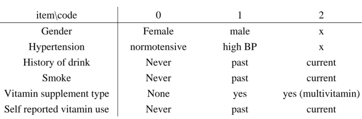
Table 3.1.2 The codebook (for discrete data)

item\code 0 1 2

Gender Female male x

Hypertension normotensive high BP x

History of drink Never past current

Smoke Never past current

Vitamin supplement type None yes yes (multivitamin) Self reported vitamin use Never past current

Table 3.1.3 The units in continuous data.

Item Unit Year of birth year

Age year Total cholesterol mg/dL

3.2

Results of numerical method

In order to simply the analysis we just select some categorical factors like smoke (the

information of package of year included), history of drinking and vitamin used and two

continuous factors age (if someone is older than 65) and year of birth (if someone is birth

before than 1922) divided each into two subgroups. The data we use is all following in four

times.

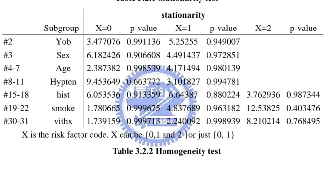
Table 3.2.1 Stationarity test

stationarity

Subgroup X=0 p-value X=1 p-value X=2 p-value

#2 Yob 3.477076 0.991136 5.25255 0.949007 #3 Sex 6.182426 0.906608 4.491437 0.972851 #4-7 Age 2.387382 0.998539 4.171494 0.980139 #8-11 Hypten 9.453649 0.663772 3.101827 0.994781 #15-18 hist 6.053536 0.913359 6.64387 0.880224 3.762936 0.987344 #19-22 smoke 1.780665 0.999675 4.837689 0.963182 12.53825 0.403476 #30-31 vithx 1.739159 0.999713 2.240092 0.998939 8.210214 0.768495

X is the risk factor code. X can be {0,1 and 2 }or just {0, 1}

Table 3.2.2 Homogeneity test

Homogeneity

times 1 p-value 2 p-value 3 p-value #2 yob 21.0670 0.00178 20.3829 0.00237 28.6282 0.00007 #3 sex 3.7381 0.71208 0.3694 0.99909 3.5203 0.74126 #4-7 age 18.2841 0.00556 18.2841 0.00556 23.7751 0.00057 #8-11 hypten 5.8456 0.44071 4.4790 0.61214 10.3536 0.11053 #15-18 hist 27.5529 0.00011 6.1372 0.40800 3.1723 0.78694 #19-22 smoke 2.7631 0.83794 13.4480 0.03645 9.3461 0.15503 #30-31 vithx 7.5825 0.27031 3.9208 0.68739 9.1054 0.16774

Table 3.2.3 the correlation of age and year of birth

age age2 age3

Although the year of birth is influential but year of birth and age are highly collinear.

The different methods [7, 8] show the birth cohort effect but in this report we do not deal

with both just select age in the model.

Finally, we select the age (x1) and history of drink (x2) in our model. The stationarity test is insignificant so we combine all the times under the Markov property assumption the

next time a participant provides a independent data. In the assumption we believe that the

risk factor would multiple the original probability then the statistical model is as following:

[ ]

(

)

⎩ ⎨ ⎧ ≠ ≠ ∀ Σ − = − − − − = = = , 2 1 0 , exp _{,0 ,1 1 ,2 2 1 2 02} i j i P x x x x P P i ij ij ij ij ij ij γ β β β P

{ }

_∑

≠ = Σ ∈ i j ij i p x x, 0,1, and where _{1 2}

0 1 2

0 1 2

0 1 2

0 1 2

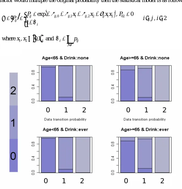
Figure 3.2.1 the transition probability of data

Figure 3.2.1 contains 4 graph illustrations of transition probabilities in each different covariate. The horizontal axes represent the starting state; the vertical axes represent the sum of the transition probability.

0 1 2

0 1 2

0 1 2

0 1 2

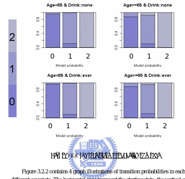
Figure 3.2.2 the transition probability of model

Figure 3.2.2 contains 4 graph illustrations of transition probabilities in each different covariate. The horizontal axes represent the starting state; the vertical axes represent the sum of the transition probability.

Table 3.2.4 mle of the parameters

( )

ˆ0

exp−β exp

( )

−βˆ₁ exp

( )

−βˆ2 exp

( )

−γˆ

(0,1) 0.0462 2.7385 0.8354 1.0572 (1,0) 0.1105 0.9449 0.8653 1.2947 (1,2) 0.0103 8.2766 1.6913 0.3695

Table 3.2.5 parameter CIs using 100 rounds each round has 5955 samples

exp

( )

−βˆ0 exp

( )

−βˆ1 exp

( )

−βˆ2 exp

( )

−γˆ

L U L U L U L U (0,1) 0.0394 0.0527 2.2240 3.2164 0.5743 1.1639 0.5662 1.8719 (1,0) 0.0874 0.1440 0.7217 1.3078 0.4228 1.3530 0.6861 2.6281 (1,2) 0.0026 0.0180 4.2324 34.6112 0.5638 10.1478 0.0439 1.2775

The underline represents significant.

Table 3.2.6 parameter CIs using 300 rounds each round has 5955 samples

exp

( )

−βˆ0 exp

( )

−βˆ1 exp

( )

−βˆ2 exp

( )

−γˆ

L U L U L U L U (0,1) 0.0397 0.0527 2.2709 3.2750 0.5304 1.1166 0.6116 1.8667 (1,0) 0.0874 0.1362 0.6922 1.2958 0.4510 1.4160 0.6125 2.8056

(1,2) 0.0026 0.0206 4.0129 30.0967 0.5638 8.4565 0.0630 1.2305

The underline represents significant.

Table 3 ounds

Each round has 5955 samples .2.7 parameter CIs using 1000 r

( )

ˆ0

exp−β exp

( )

−βˆ₁ exp

( )

−βˆ₂ exp

( )

−γˆ

L U L U L U L U (0,1) 0.0397 0.0531 2.2604 3.3016 0.5338 1.1852 0.5939 1.7702 (1,0) 0.0823 0.1362 0.6824 1.3293 0.4510 1.4025 0.5698 2.8269

(1,2) 0.0026 0.0180 4.2637 32.3540 0.5638 6.7652 0.0595 1.1562

3.3

Interpretation

Since the stationarity test is insignificant so we combine the different times to analysis

and reduce the model to stationary model. Some probability is too small like (0,2) , (2,1),

(2,2) so we assumption they are 0 in the model.

The testing data is used the all following that means no missing data in the data set

and the total is 927 in three transient times . Once we select the factors then we used the no

missing data just in the interesting factors so the number of data is increasing the total is

1985.

Before generate the CIs see Figure 3.2.1 the transition probability plot show that the

history of drink is insignificant by compare with the factor present or not. With the Table

form 3.2.5 to 3.2.7 it is consist with the figure.

Some factors are effect in previous paper but they are not significant this. The reason

may be some factors affect the ARM in part and the test is over all testing so they become

not significant.

From the mle estimate we can see that the age will 2.7385 times from ARM free to

early-ARM and 8.2766 times form early-ARM to late-ARM. Beside it seems to prevent

from early-ARM to ARM free (0.9449 times but not significant).

In the common scene we may think the elder and the worse the ARM. In fact, age will

4 Conclusion

In this report we develop a new analysis of transition data with factors. Under the

Markov property assumption we can easily solve the dependent data question but we need

an “enough” sample size the better is uniform in each cell of probability. Use this method

we will have a global view of a disease different from other methods in the past.

We use the ARM data to demonstrate the method in this example age happened to a

factor so we do not need to develop a non-stationary model of course we can do it also.

The parametric model you can try any reasonable intuitively for factors and disease.

It’s quite flexible.

The future work may try to develop a continuous time Markov chain with factors in

5

Reference

1. A randomized, placebo-controlled, clinical trial of high-dose supplementation with vitamins C and E, beta carotene, and zinc for age-related macular degeneration and vision loss. Age-related Eye Disease Study Research Group. Arch Ophthalmol 2001;119 1417–36. (AREDS report no. 8).

2. Allain CC, Poon LS, Chan CGS, et al. Enzymatic determination of total serum cholesterol. Clin Chem 1974;20 470–5.

3. Basawa, Rao, Statistical Inference for Stochastic Process.

4. B. F. Efron, Bootstrap Methods: Another Look at the Jackknife. Ann. Statist. 1979;

7 1-26.

5. B. F. Efron, Computers and the Theory of Statistics: Thinking the unthinkable. SIAM

Review . 1979; 21 460-480.

6. George Casella, Roger L. Berger. Statistical Inference 2001

7. Huang GH, Ronald Klein, Barbara E. K. et al.Birth Cohort Effect on Prevalence of Age-related Maculopathy in the Beaver DamEye Study.

Am J Epidemiol 2003;157 721–729

8. Huang GH, Klein R, Klein BEK: Joint analysis of incidence, progression, regression and disappearance rates. Manuscript

9. Klein R, Klein BEK, Linton KLP, et al. The Beaver Dam Eye Study: visual acuity.

Ophthalmology 1991;98 1310–15.

10. Klein R, Klein BEK, Franke T. The relationship of cardiovascular disease and its risk factors to age-related maculopathy. The Beaver Dam Eye Study. Ophthalmology 1993;100 406–14.

11. Klein R, Klein BEK, Lee KP. The changes in visual acuity in a population. The Beaver Dam Eye Study. Ophthalmology 1996; 103 1169–78.

12. Klein R, Klein BEK, Moss SE. Relation of smoking to the incidence of age-related maculopathy: the Beaver Dam Eye Study. Am J Epidemiol 1998; 147 103–10.

13. Klein R, Klein BEK, Lee KE, et al. Changes in visual acuity in a population over a 10-year period: the Beaver Dam Eye Study. Ophthalmology 2001;108 1757–66.

14. Klein R, Klein BEK, Tomany SC, et al. Ten-year incidence of age-related

maculopathy and smoking and drinking: the Beaver Dam Eye Study. Am J Epidemiol 2002; 156 589–98.

15. Klein R, Klein REK, Wong TY, Tomany SC, Cruickshanks KJ. The association of cataract and cataract surgery with the long-term incidence of age-Related maculopathy.

Archives of Ophthalmology 2002; 120 1551-1558.

16. Klein R, Klein BEK, Tomany SC, et al. The association of cardiovascular disease with the long-term incidence of age-related maculopathy. The Beaver Dam Eye Study.

Ophthalmology (in press).

17. Linton KLP, Klein BEK, Klein R. The validity of self-reported and surrogate-reported cataract and age-related macular degeneration in the Beaver Dam Eye Study. Am J

Epidemiol 1991; 134 1438–46.

18. S. Ross, Stochastic Process, 2nd Wiley.

19. The hypertension detection and follow-up program. Hypertension Detection and Follow-up Program Cooperative Group. Prev. Med. 1976; 5 207–15.