國 立 交 通 大 學
管 理 學 院
企業管理碩士學位學程
碩 士 論 文
金融風暴前後汽車及零組件產業之
永續競爭優勢族群分析
An Empirical Study of
Configuring Competitive Advantages for Sustainable Growth
in Automobile Industry before and after financial crisis
研 究 生:徐瓊璐
指導教授:唐瓔璋博士
金融風暴前後汽車及零組件產業之
永續競爭優勢族群分析
An Empirical Study of
Configuring Competitive Advantages for Sustainable Growth
in Automobile Industry before and after financial crisis
研
究 生 :徐瓊璐
Student: Chiung-Lu Hsu
指導教授:唐瓔璋博士 Advisor: Dr. Ying-Chan Tang
國
立 交 通 大 學
管理學院
企業管理碩士學位學程
碩
士 論 文
A Thesis
Submitted to Master Degree Program of Global Business Administration
College of Management
National Chiao Tung University
in partial Fulfillment of the Requirements
for the Degree of
Master
in
Business Administration
July 2014
Hsinchu, Taiwan, Republic of China
金融風暴前後汽車及零組件產業之
永續競爭優勢族群分析
研
究 生 :徐瓊璐
指導教授:唐瓔璋博士
國
立 交 通 大 學
管理學院
企業管理碩士學位學程
碩
士 論 文
Chinese Abstract 中文摘要
在全球化的動態競爭局勢下,如何保持企業組織的永續競爭力儼然成為學術 研究的顯學。本研究試圖嘗試利用研究金融風暴前後三年內的汽車及其零組件產業的 財務報表,從中推演出汽車及零組件產業的關鍵競爭優勢並依據將此產業進行優勢分 群。本研究發現在金融風暴前,本產業可以劃分為流程效率優勢族群、技術創新族群 及資產利用優化族群。金融風暴後,不令人驚奇的發現此時期的優勢族群稍有變化, 但是競爭優勢的特質與前期大致雷同,此時期的產業被劃分為流程效率優勢族群,雙 手同能族群,及資產利用優化族群。本研究將前後兩時期的策略族群交叉比較,進一 步依據金融風暴前後的策略優勢轉折將此產業內的公司細分為九種型態。最後使用變 異數分析分析此九種型態的財務績效後發現,此九種型態族群的資本投資報酬率 (ROIC),在 95%的信心水準的統計驗證上被證實有顯著差異。其中危機前期屬於技 術創新,危機後期屬於雙手同能的第八型態族群的財務績效顯著優於以下四種族群: 一、 兩期都是效率流程優勢族群,二、兩期都是產能利用優化族群,三、前期產能 利用優化後期流程效率優勢的族群以及四、前期產能利用優化後期雙手同能的族群。 本研究總結前後期研究發現,主導汽車產業的關鍵競爭力可歸納為以下四種:高績效 的流程管理能力,資產利用優化能力,創新科技的續航力以及雙元組織能力的均衡發 展。 關鍵字:競爭優勢 雙元組織 策略族群 杜邦方程式 汽車及其零組件產業 iAn Empirical Study of
Configuring Competitive Advantages for Sustainable Growth
in Automobile Industry before and after financial crisis
Student: Chiung-Lu Hsu Advisors: Dr. Ying-Chan Tang
Master Degree Program of Global Business Administration
College of Management
National Chiao Tung University
English Abstract
This research applied financial ratio to configure the competitive advantages and prevailing strategies in the automobile industry before and after financial crisis. The decomposed financial ratio revealed the resources allocation of the firms and implicitly indicated the possible strategies the firms applied. Four factors were derived to represent as critical resource allocation before crisis, which were Administration Process Efficiency, Assets Utilization Arrangement, External Relationship and Technology Exploration. Ambidextrous Value Creation, Assets Utilization Arrangement and Relationship Leverage, three factors were derived from the financial index in the period of after crisis. In each period, three strategic groups were clustered based on the latent resource allocation types and each group was salient with its unique competitive advantages. Before financial crisis, the automobile industry was classified into Process Efficiency group, Assets Utilization group and Technology Exploration group. The strategic groups were Process Efficiency, Ambidexterity Prone and Assets Utilization after financial crisis. Further compared the two classifications by cross tabulation of the clustering groups in two periods and resulted in 9 types of strategy swift of competitive advantages. At 95% confidence interval, there was significant difference between the 9 types and financial performance represented by ROIC. Furthermore, Type 8, which originated at Technology Exploration groups and switched to Ambidexterity Prone groups, appealed to create higher profits than other 4 types of groups (Type 1, 4, 5 and 6). In the end, the two classifications of strategic groups in two periods plausibly summarized to four dominant competitive advantages in the automobile industry.
1. Capability of managing Process Efficiency; 2. Capability of maximizing Assets Utilization ; 3. Capability of insisting on Technology Exploration; 4. Capability of balancing Ambidexterity Prone.
Keywords: Competitive advantage, Organizational ambidexterity, Strategic Group, Du Pont identifier, Automobile industry
Acknowledgement
I would like to express my sincere appreciation and thanks to my advisor Dr. Ying-Chan Tang, who has been a tremendous mentor for me. I would like to thank for his encouraging my research and fostering me to grow as an independent research thinker. His advice on both research as well as on my career have been priceless. I would also like to thank my committee members, Dr. Jin-Li Hu and Dr. Mei-Fang Chen, for serving as my committee advisors even at hardship. I also want to thank for their valuable comments and suggestions to further polish my thesis.
A special thanks to my family. Words cannot express how grateful I am to my father, my mother, my brothers, my sisters in law and my baby sister for all of the sacrifices that they have made on my behalf. Their kind prayers and full assistance for me were what supported me to strive toward my goal. I would also like to thank all of my friends who supported me and encouraged me during my hard time. At the end I would like express appreciation to my beloved husband, Warren, who spent sleepless nights with me and his consent and supports for me sustained me thus far.
Sincerely,
Lucy Hsu 2014/8/12
Table of Contents
Chinese Abstract 中文摘要 ... i English Abstract ... ii Acknowledgement ... iii Research motivation ... 1 Literature review ... 2 2.1 Competitive advantage ... 2 2.2 Dynamic capability ... 32.3 Organizational configuration and strategic group ... 3
2.4 Organizational ambidexterity ... 4 2.5 Du Pont identifier ... 4 Research methodology ... 5 3.1 Research parameters ... 5 3.2 Analytical process ... 6 3.3 Research methods ... 6 Research results ... 8 4.1 Samples ... 8
4.2 Principal component analysis results ...10
4.3 Cluster analysis results ...15
4.4 Discriminant analysis results ...19
4.5 Cross tabulation comparison for categorical variables ...22
4.6 ANOVA test on ROIC and EBIT rate among clusters ...26
4.7 Strategy transition ...27
4.8 ANOVA test for 9 types of strategy transitions ...28
Conclusion ...29
Research limitation ...30
Research contribution ...31
Bibliographies ...32
Appendix 1 Firms in nine types of strategy transition ...33
Autobiography ...35
Tables
TABLE 1RESEARCH PARAMETERS ... 5
TABLE 2ROIC TREND IN AUTOMOBILE INDUSTRY FROM 2007 TO 2012 ... 8
TABLE 3DESCRIPTIVE STATISTICS FOR TWO PERIODS ... 9
TABLE 4ROTATED FACTOR PATTERN BEFORE FINANCIAL CRISIS ... 11
TABLE 5ROTATED FACTOR PATTERN AFTER FINANCIAL CRISIS ... 13
TABLE 6CRITERIA OF OPTIMAL NUMBER OF CLUSTERS ... 15
TABLE 7AVERAGED FACTOR SCORES IN EACH CLUSTER BEFORE CRISIS ... 15
TABLE 8AVERAGED FACTOR SCORES IN EACH CLUSTER AFTER CRISIS ... 17
TABLE 9RESULTS OF DISTRIMINANT ANALYSIS BEFORE CRISIS. ... 19
TABLE 10RESULTS OF DISCRIMINANT CANONICAL FUNCTION BEFORE CRISIS ... 19
TABLE 11HIT RATIOS OF DISCRIMINANT ANALYSIS AND CROSS VALIDATION BEFORE CRISIS ... 20
TABLE 12RESULTS OF DISCRIMINANT ANALYSIS AFTER CRISIS ... 20
TABLE 13RESULTS OF DISCRIMINANT CANONICAL FUNCTION AFTER CRISIS ... 21
TABLE 14HIT RATIOS OF DISCRIMINANT ANALYSIS AND CROSS VALIDATION AFTER CRISIS ... 21
TABLE 15TABLE OF CLUSTER BY SIC ... 22
TABLE 16TABLE OF COUNTRY BY CLUSTER IN TWO PERIODS ... 23
TABLE 17TABLES OF REGION BY CLUSTER ... 23
TABLE 18TABLE OF CLUSTER BY EMPLOYEE SIZE ... 23
TABLE 19TABLE OF CLUSTER BY ROICD ... 24
TABLE 20TABLE OF EBIT_SD BY CLUSTERS ... 24
TABLE 21TABLE OF AMB_RS BY CLUSTERS ... 25
TABLE 22ANVOA TEST OF ROIC AND EBIT_S ... 26
TABLE 23CROSS COMPARISON OF TWO CLUSTERING ... 27
TABLE 24ANOVA TEST IN ROIC&EBIT_S FOR 9 TYPES OF STRATEGY TRANSITIONS ... 28
Figure
FIGURE 1ANALYTICAL PROCESS OF THE RESEARCH ... 6FIGURE 2ROIC TREND OF SAMPLE FIRMS IN AUTOMOBILE INDUSTRY ... 8
FIGURE 3COMPARISON OF FACTOR SCORES MEAN AMONG CLUSTERS BEFORE CRISIS ... 16
FIGURE 4COMPARISON OF FACTOR SCORES MEAN AMONG CLUSTERS AFTER CRISIS ... 17
Research motivation
In the trend of dynamic competition and globalization, the issue of sustainable growth of organizations has been one of the major research topics in the academic industry. Classical strategic management theory claimed that an organization with extinguished competitive advantages promisingly entailed its sustainable growth (Barney, 1991; Porter 1985). However the heterogeneous performance occurred among organizations which used to be marked with competitive advantages. Powell proposed a new perspective to explain the difference. He elaborated that not only competitive advantages but also organizational errors of an organization could result eminent influence on its performance (Powell & Arregle 2007; Tang & Liou 2010). March (1990) defined the competitive advantages from organizational learning’s point of view as exploitation and exploration. If the firms who were capable of balancing the capabilities of exploitation and exploration, the firms were classified as ambidextrous organizations. Firms that cannot balance the capability of exploitation and exploration were defined as committing organizational errors. In recent years, the theory of organizational ambidexterity led a new research paradigm in
organization theory and more researches regarded organizational ambidexterity as one of the key factors to maintain competitive advantages in a quick-changed environment.
The research was aimed to study of how to use financial figures to address competitive advantages and how to apply organization financial performance, resource configuration, and organizational ambidexterity to analyze the evolutionary changes of automotive industry from 2007 to 2012. The research further tried to verify if
organizational ambidexterity could be proved to positively influence superior financial performance of an organization in the long-term.
Literature review
Traditional competitive theory believed that competitive advantages were the key elements of maintaining organizational sustainable performance. However, some successful organizations who once outperformed in their era suffered while encountering discontinuity environment changes. Researchers initialed relative studies to find out possible reasonable causes of maintaining the sustainable performance. In this atmosphere, organizational ambidextrous theory was one of the prevailed contemporary theories applied to address the capability of maintaining superior performance. Ambidexterity related theory declared that the organizations that were capable of balancing the competitive advantages of exploitation and exploration at the same time should be likely to enjoy the outperforming growth.
2.1 Competitive advantage
Porter proposed that competitive structure of an industry was the main force of influencing the organizational performance. Porter further identified two basic types of competitive advantages, cost leadership and differentiation, which firms could exercise according to their positions in the industry structure. The cost leadership competitive advantage existed as a firm offered the same value to customers with lower cost and the differentiation advantages emerged as a firm offered more valued benefits to customers with similar products or service.
Resource-based view defined competitive advantages as the firm’s ability to efficiently create or preserve scarce resources to outperform its competitors. This ability could be achieved by appropriate resource allocation (Reed, 1990). Even though
competitive advantages may be duplicated through the resource distribution of a company, heterogeneous performance still occurred among organizations which once carried similar competitive advantages.
March redefined the competitive advantages from the view of organizational learning theory by proposing two new competitive advantages, exploitation and exploration, to emphasize the organizations’ ability of creating values (March, 1991). Exploitation represented the ability to make the best usage of current resources, in terms of activities related to operational efficiency, duplication or execution, whereas exploration advantages represented the ability to explore new opportunities, in terms of activities related to developing new technologies, new businesses and new production technologies. (March, 1991). Utila et. al (2009) also proved that there was curved linear relationship between sales performance and exploration behaviors.
Along with the quick-changes in the global business, the static competitiveness view
was criticized to fail into simplicity and logic tautology (Tang, 2010). Teece, Pisano, and Shuen(1997) proposed dynamic capability theory to address a firm’s capability that should be altered according to the changes of environment.
2.2 Dynamic capability
Dynamic capability was defined by Teece et al. (1997) as "the firm’s ability to integrate, build, and reconfigure internal and external competences to address rapidly changing environments." Teece’s concept of dynamic capabilities essentially declared that competitiveness derived from enhancing, combining, protecting, and, when necessary, reconfiguring the enterprise’s intangible and tangible assets.” In other words, dynamic capability was applied to address a firm’s ability to maintain competitive survival especially when facing changes.
Zott(2003) proposed that the firm’s dynamic capability indeed made influence on its performance. The cultivation timing, imitation of competitors’ resource allocation,
developing and learning cost and utilization of dynamic capability were all critical to the firms’ integral performance and were also responsible for the diversity of performance.
2.3 Organizational configuration and strategic group
Zott(2003) proposed that the dynamic capability derived from the process when a firm allocated its resources and each firm created its own unique resource configuration based on its corporate strategy and management ability. The concept of resource
configuration was similar to the concept of organizational configuration in organizational theory. The organizational configuration was an organizational framework used to explain how an organization was shaped in a certain way and why some organizations shared similar characters or frameworks (Mintzberg 1990, Meyer et al., 1993).
Tang and Liou (2010) redefined the causal relationship between the sustainable competitiveness and superior performance as strategy, resource, configuration and
performance. They declared that cooperate strategy determined a firm’s resource allocation and a firm’s resource allocation would eventually shape its organizational resource
configuration, which implied the latent competitive advantages of the company. The latent competitive advantages ended up influencing the firm’s performance. In other words, a firm’s competitive advantages were cultivated by its resources allocation and organizational configuration.
Hunt(1972) proposed the concept of strategic group in his study of competition in the major home appliance industry. He discovered the existence of subgroups within the same industry and the competition level within a subgroup was fiercer than level from
industry average. Different subgroups competed with different combinations of strategies. Strategic group analysis was the application of taxonomy method, where the subjects were classified empirically by their analogue functions (Mayr,1969).
Cool and Schendel (1987) believed that strategic groups was classified for
distinguishing those who owned similar strategy combinations or resource allocation within the same industry and directly competed with one another. In other words, the different strategic groups owned different resource configuration.
2.4 Organizational ambidexterity
March (1991) referred that a firm’s capability of balancing both exploitation and exploration advantage simultaneously improved its chance of maintaining sustainable performance. The capability was further defined as organizational ambidexterity and was applied to explain why some organizations could continue their super performance not only when facing gradually incremental evolutionary change, but also when dealing with
revolutionary changes within the quick-changing dynamic environment (Tushman & O’Reilly, 1997). Gibson and Birkinshaw further proved that there was positive relationship between ambidexterity and firms’ financial performance. (Gibson & Birkinshaw, 2004)
2.5 Du Pont identifier
Du Pont identifier was the one of the substantial financial index which could be fairly addressed the relationship between financial performance and resource inputs. Du Pont identifier was broadly applied to decompose a firm’s capacity, especially to configure the ability of generating profits and utilizing resources. Grant (2008) used Du Pont identifier to decompose ROIC into several financial index such as SGA/sales, COGS/sales,
depreciation/sales and Fixed assert turnover rate to analyze Ford automobile. Tang and Liou (2010) also applied Du Pont identifier to configure strategic groups in semiconductor industry. (Financial index: Account receivable turnover rate, Tax/sales and inventory turnover rate.) Return on invested capital (ROIC) was considered as good index to measure a firm’s performance and its ability of creating profits for stockholders (Cao, Jiang and Koller, 2006). 𝐑𝐑𝐑𝐑𝐑𝐑𝐑𝐑 =𝑬𝑬𝑬𝑬𝑬𝑬 ×𝑵𝑵𝑵𝑵 𝑬𝑬𝑬𝑬𝑵𝑵𝑬𝑬 ×𝑬𝑬𝑬𝑬𝑬𝑬 𝑺𝑺𝑺𝑺𝑺𝑺𝑺𝑺𝑺𝑺 ×𝑬𝑬𝑬𝑬𝑵𝑵𝑬𝑬 𝑺𝑺𝑺𝑺𝑺𝑺𝑺𝑺𝑺𝑺𝑬𝑬𝑻𝑻 ×𝑬𝑬𝑻𝑻𝑵𝑵𝑰𝑰 (1) 𝐑𝐑𝐑𝐑𝐑𝐑𝐑𝐑 = 𝐓𝐓𝐓𝐓𝐓𝐓 𝐁𝐁𝐁𝐁𝐁𝐁𝐁𝐁𝐁𝐁𝐁𝐁 𝐓𝐓 𝐑𝐑𝐁𝐁𝐈𝐈𝐁𝐁𝐁𝐁𝐁𝐁𝐈𝐈𝐈𝐈 𝐁𝐁𝐁𝐁𝐁𝐁𝐁𝐁𝐁𝐁𝐁𝐁 𝐓𝐓 𝐄𝐄𝐁𝐁𝐑𝐑𝐓𝐓 𝐌𝐌𝐓𝐓𝐁𝐁𝐌𝐌𝐌𝐌𝐁𝐁 𝐓𝐓 𝐀𝐀𝐈𝐈𝐈𝐈𝐁𝐁𝐈𝐈 𝐓𝐓𝐁𝐁𝐁𝐁𝐁𝐁𝐓𝐓𝐓𝐓𝐁𝐁𝐁𝐁 𝐓𝐓 𝐋𝐋𝐁𝐁𝐓𝐓𝐁𝐁𝐁𝐁𝐓𝐓𝐌𝐌𝐁𝐁 (2) 4
Research methodology
3.1 Research parameters
This research revised the definition of the Du Pont identity from Tang and Liou(2010) and added new variables, the ratio of interest over sales, to further take the interests effect into consideration. The financial index indicated the firm’s capability of manipulating its resource to create value for the company. ROIC and EBIT margin was employed to represent a firm’s overall performance, EBIT margin was the ratio of Earnings before interest and tax over sales and it represented the power of a firm’s core competence of generating profits.
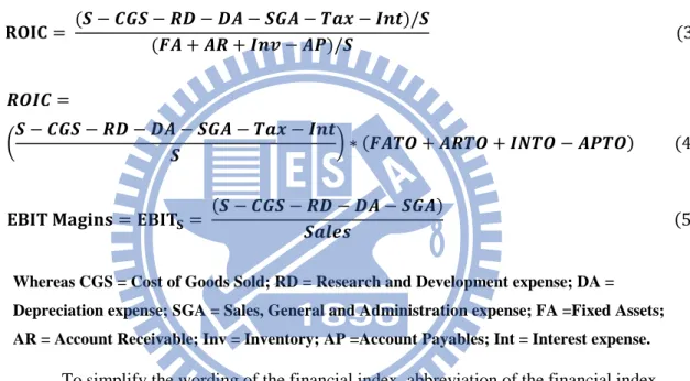
𝐑𝐑𝐑𝐑𝐑𝐑𝐑𝐑 = (𝑺𝑺 − 𝑰𝑰𝑪𝑪𝑺𝑺 − 𝑹𝑹𝑹𝑹 − 𝑹𝑹𝑻𝑻 − 𝑺𝑺𝑪𝑪𝑻𝑻 − 𝑬𝑬𝑺𝑺𝑻𝑻 − 𝑵𝑵𝑰𝑰𝑰𝑰)/𝑺𝑺(𝑭𝑭𝑻𝑻 + 𝑻𝑻𝑹𝑹 + 𝑵𝑵𝑰𝑰𝑰𝑰 − 𝑻𝑻𝑨𝑨)/𝑺𝑺 (3) 𝑹𝑹𝑹𝑹𝑵𝑵𝑰𝑰 =
�𝑺𝑺 − 𝑰𝑰𝑪𝑪𝑺𝑺 − 𝑹𝑹𝑹𝑹 − 𝑹𝑹𝑻𝑻 − 𝑺𝑺𝑪𝑪𝑻𝑻 − 𝑬𝑬𝑺𝑺𝑻𝑻 − 𝑵𝑵𝑰𝑰𝑰𝑰𝑺𝑺 � ∗ (𝑭𝑭𝑻𝑻𝑬𝑬𝑹𝑹 + 𝑻𝑻𝑹𝑹𝑬𝑬𝑹𝑹 + 𝑵𝑵𝑵𝑵𝑬𝑬𝑹𝑹 − 𝑻𝑻𝑨𝑨𝑬𝑬𝑹𝑹) (4) 𝐄𝐄𝐁𝐁𝐑𝐑𝐓𝐓 𝐌𝐌𝐓𝐓𝐌𝐌𝐌𝐌𝐁𝐁𝐈𝐈 = 𝐄𝐄𝐁𝐁𝐑𝐑𝐓𝐓𝐒𝐒= (𝑺𝑺 − 𝑰𝑰𝑪𝑪𝑺𝑺 − 𝑹𝑹𝑹𝑹 − 𝑹𝑹𝑻𝑻 − 𝑺𝑺𝑪𝑪𝑻𝑻)𝑺𝑺𝑺𝑺𝑺𝑺𝑺𝑺𝑺𝑺 (5)
Whereas CGS = Cost of Goods Sold; RD = Research and Development expense; DA = Depreciation expense; SGA = Sales, General and Administration expense; FA =Fixed Assets; AR = Account Receivable; Inv = Inventory; AP =Account Payables; Int = Interest expense.
To simplify the wording of the financial index, abbreviation of the financial index was named as below table 1 and used in the context of the research.
Table 1 Research parameters
Financial
index Definition
Financial
index Definition
APTO Account payable Turnover Rate ROIC Return of Invested Capital
ARTO Account Receivable Turnover Rate EBIT_S the ratio of Earnings Before Interest and Tax over sales IN_TO Inventory Turnover Rate ROICD compared single firm's ROIC with industry average
FATO Fixed Assets Turnover Rate EBIT_SD compared single firm's EBIT_S with industry average RD_S the ratio of R&D expense over sales AMB_RS Both RD_S & SGA_S larger than industry average SGA_S the ratio of SGA expense over sales EMP Employees numbers
C_S the ratio of CGS expense over sales(CGS_S) DA_S the ratio of Depreciation expense over sales TAX_S the ratio of Tax expense over sales
INT_S the ratio of Interest expense over sales
Research parameters
3.2 Analytical process
Below chart represented the analytical process of the research.
Figure 1 Analytical process of the research
3.3 Research methods
Below listed the methods applied in the research:
(1) Descriptive Statistics of DuPont identifiers financial index
(2) Principal component analysis
(3) Cluster analysis
(4) Discriminant Analysis
(5) Cross tabulation
(6) ANOVA test
This research aimed to compare the strategic groups’ changes before and after the financial crisis. Financial index derived from Du Pont identifiers were manipulated as basic variables and the descriptive statistics was calculated to summarize the sample data.
Next, the research ran principal component analysis to simplify the financial variables into latent factors which were deployed to represent the hidden resources configuration of firms in the industry.
In the next step, the research adapted these latent factors to run cluster analysis and grouped firms in each period. Meanwhile, the research followed up applying the
discriminant analysis to verify the effectiveness of the grouping.
After finalizing the clusters, cross tabulation comparison was used to address the characteristics of clusters and ANOVA test was applied to examine the financial performance (ROIC EBIT_S) of each cluster.
In the end, the research further analyzed the strategy swift of the firms before and after financial crisis and resulted in nine types of strategy transition for automobile industry. The transitions were analyzed to explain how firms adjusted the resource allocation before and after the financial crisis and how the performance they ended in. Thus, ANOVA test was applied to further test the financial performance of the type of strategy transitions.
In the research, the ratio of SGA expense over sales was assumed to represent the exploitation advantages of an organization and the ratio of RD expense over sales was used to address the exploration advantage. The performance index of an organization was represented by the ratio of ROIC and EBIT_S. The companies whose SGA_S and RD_S were both higher than industry average were defined as ambidextrous organizations. If either value of a firm was lower than industry average, the firm was considered as not with ambidexterity.
Research results
4.1 Samples
The research boundary was limited in the companies which had 6 years averaged financial ratio dated from 2007 to 2012 and the companies was classified in Motor Vehicles & Passenger Car Bodies(SIC:3711) and Motor Vehicle Parts & Accessories(SIC:3714). The financial data was collected from S&P COMPUSTAE Database.
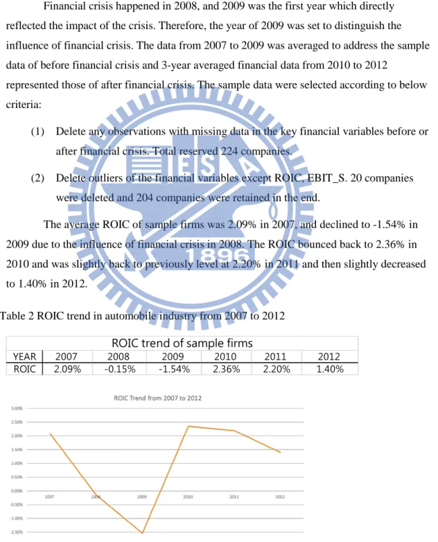
Financial crisis happened in 2008, and 2009 was the first year which directly reflected the impact of the crisis. Therefore, the year of 2009 was set to distinguish the influence of financial crisis. The data from 2007 to 2009 was averaged to address the sample data of before financial crisis and 3-year averaged financial data from 2010 to 2012
represented those of after financial crisis. The sample data were selected according to below criteria:
(1) Delete any observations with missing data in the key financial variables before or after financial crisis. Total reserved 224 companies.
(2) Delete outliers of the financial variables except ROIC, EBIT_S. 20 companies were deleted and 204 companies were retained in the end.
The average ROIC of sample firms was 2.09% in 2007, and declined to -1.54% in 2009 due to the influence of financial crisis in 2008. The ROIC bounced back to 2.36% in 2010 and was slightly back to previously level at 2.20% in 2011 and then slightly decreased to 1.40% in 2012.
Table 2 ROIC trend in automobile industry from 2007 to 2012
Figure 2 ROIC trend of sample firms in automobile industry
YEAR 2007 2008 2009 2010 2011 2012
ROIC 2.09% -0.15% -1.54% 2.36% 2.20% 1.40%
ROIC trend of sample firms
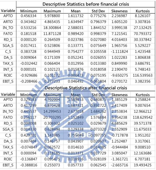
Below was the table of the descriptive statistics about the sample data.
Table 3 Descriptive statistics for two periods
Minimum Maximum Mean Std Dev Skewness Kurtosis
APTO 0.456334 5.978800 1.611732 0.775276 2.236987 8.126107 ARTO 0.343462 4.865435 1.634947 0.796379 1.605120 3.307816 IN_TO 0.533216 18.300864 2.588031 1.844152 3.999138 27.132425 FATO 0.181518 11.871128 0.989420 0.998379 7.121541 70.793372 RD_S 0.000120 0.264509 0.023786 0.027080 4.016403 30.337842 SGA_S 0.017411 0.523806 0.133771 0.075649 1.965756 5.529227 C_S 0.383728 0.944949 0.754277 0.105558 -1.111824 1.423548 DA_S 0.009064 0.171309 0.052241 0.026055 1.022283 1.806838 TAX_S -0.032442 0.066404 0.012956 0.013380 0.849990 3.686791 INT_S 0.000101 0.102123 0.015876 0.018058 2.190470 5.748143 ROIC -0.929686 0.101172 0.000473 0.075195 -9.650275 116.539563 EBIT_S -0.208466 0.277233 0.046492 0.061804 0.270172 3.382356
Minimum Maximum Mean Std Dev Skewness Kurtosis
APTO 0.329183 4.702004 1.589853 0.680875 1.385129 3.258824 ARTO 0.417299 6.870428 1.687321 0.891722 2.417409 9.007654 IN_TO 0.445537 14.299453 2.677018 1.684262 2.753834 12.966212 FATO 0.256117 20.703295 1.152849 1.576884 9.954238 118.629542 RD_S 0.000008 0.306932 0.025102 0.029679 4.685629 39.571378 SGA_S 0.014330 0.628494 0.129338 0.073320 2.552909 11.675033 C_S 0.429701 1.141985 0.755649 0.097755 -0.717878 1.951202 DA_S 0.007404 0.146757 0.043907 0.020637 1.252487 3.317061 TAX_S -0.074847 0.062572 0.014610 0.014085 -0.944484 9.008510 INT_S 0.000094 0.118185 0.013371 0.017729 3.085047 12.163686 ROIC -0.136847 0.095475 0.018916 0.028109 -1.361721 6.707181 EBIT_S -0.388816 0.255073 0.057733 0.062545 -2.665716 19.493425 Descriptive Statistics before financial crisis Descriptive Statistics after financial crisis Variable Variable 9
4.2 Principal component analysis results
The research adopted 10 financial figures decomposed from Du Pont identifiers to represent the resource bundles in the automobile industry. The financial variables were applied to run PCA analysis and common latent factors were derived to represent the latent factors prevailing around the automobile industry in each period. These key latent factors also addressed the resource combinations which further shaped the characteristic of the competitive advantages required by the industry (Tang & Liou, 2010).
The main purpose of applying principal component analysis (PCA) was to reduce the variables numbers. PCA not only drew new synthetic variables underlying the original resource bundles, but also kept the contents of the original information. Secondly, these new variables were mutually independent and the independent characteristics offset the issue of multicollinearity in the analysis of financial index.
The KMO values of 10 financial variables before and after financial crisis were 0.51 and 0.56 accordingly. Both KMO values were larger than 0.5, and the values entailed the appropriateness of the variables for principal component analysis.
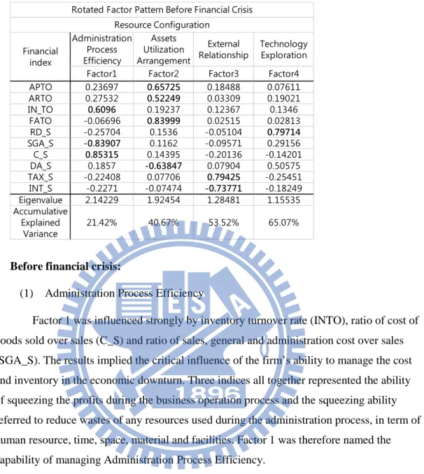
The research applied the criteria suggested by Zateman and Burger (1975) for judging the significance of factor analysis: the eigenvalue of latent factors is larger than 1, the accumulative explanation variance is larger than 40% and the factor loadings after varimax rotation are considerably significant if they are larger than 0.3. According to the table of rotated factor pattern before financial crisis, four factors were selected because their eigenvalues were larger than 1 and the accumulative explained variation of four factors were up to 65%. Likewise, three factors were derived after financial crisis based on the same criteria, but its accumulative explained variation was slightly lower, which was 54%.
The nomination for the latent factors was mainly affected by the loadings of the rotated factor pattern derived from varimax method. In this research, if the loadings of the variables were larger than 0.5, the variables were considered to be significant to that factor and the factor would be given a name depending on the interactive influence of these variables. In next paragraph, the research further elaborated the reasoning about the nomination of each factor before and after the financial crisis.
Table 4 Rotated factor pattern before financial crisis
Before financial crisis:
(1) Administration Process Efficiency
Factor 1 was influenced strongly by inventory turnover rate (INTO), ratio of cost of goods sold over sales (C_S) and ratio of sales, general and administration cost over sales (SGA_S). The results implied the critical influence of the firm’s ability to manage the cost and inventory in the economic downturn. Three indices all together represented the ability of squeezing the profits during the business operation process and the squeezing ability referred to reduce wastes of any resources used during the administration process, in term of human resource, time, space, material and facilities. Factor 1 was therefore named the capability of managing Administration Process Efficiency.
(2) Assets Utilization Arrangement
Factor 2 was dominated by account payable turnover rate (APTO), account receivable turnover rate (ARTO), fixed assets turnover rate (FATO) and ratio of
depreciation cost over sales (DA_S). These variables were related to assets and production efficiency and therefore factor 2 was named as capability of Assets Utilization
Arrangement.
DA_S and factor 2 were negatively related. The higher the DA_S was the less influence of the factor 2 was. If the firms invested more in facilities or equipment, its higher DA_S lowered the value of Assets Utilization Arrangement. On the contrary, the FATO and factor2 were positively related, and therefore if FATO was higher, the value of factor 2 would also be higher. APTO and ARTO here were viewed as kinds of relationship assets.
Administration Process Efficiency Assets Utilization Arrangement External
Relationship TechnologyExploration
Factor1 Factor2 Factor3 Factor4
APTO 0.23697 0.65725 0.18488 0.07611 ARTO 0.27532 0.52249 0.03309 0.19021 IN_TO 0.6096 0.19237 0.12367 0.1346 FATO -0.06696 0.83999 0.02515 0.02813 RD_S -0.25704 0.1536 -0.05104 0.79714 SGA_S -0.83907 0.1162 -0.09571 0.29156 C_S 0.85315 0.14395 -0.20136 -0.14201 DA_S 0.1857 -0.63847 0.07904 0.50575 TAX_S -0.22408 0.07706 0.79425 -0.25451 INT_S -0.2271 -0.07474 -0.73771 -0.18249 Eigenvalue 2.14229 1.92454 1.28481 1.15535 Accumulative Explained Variance 21.42% 40.67% 53.52% 65.07% Financial index Resource Configuration
Rotated Factor Pattern Before Financial Crisis
The relationship assets controlled the ability to bargain over suppliers or customers. Therefore, if the APTO and ARTO were higher, the value of Assets Utilization Arrangement factor was higher as well.
(3) External Relationship
The ratio of tax over sales (TAX_S) and the ratio of interests over sales (INT_S) demonstrated significant influence on the factor 3. Tax was considered as the investment from the government and interests was the cost of utilizing capital borrowed from the creditors. Both the creditors and government involved with the profits outflow of the company. In this point of view, both parties were regarded as external investors for the company. If the INT_S was higher, it implied that the firms owned substantial debt which further suggested the firm’s strong relationship with creditors, such as banks. Higher interest expense was likely to indirectly reduce the tax expense because of the effect of tax shield.
On the other hand, if the firm was taxed significantly, it indicated the firm owned strong relationship with government, and the firm might have more influence to acquire supports from the government. With regard to above reasoning, the factor 3 was named as factor of managing External Relationship.
(4) Technology Exploration
Because only the loadings of RD_S was significantly larger than 0.5, it was not easy to give a name for the factor 4. However, the factor explained significantly 11% of variance for the sample data and RD_S variable played an important role in this research. Therefore, the research boldly named factor 4 as the capability of Technology Exploration.
In the economic downturn, most companies paid attention on the budget control and cost-down arrangement in respect of the decrease of sales. If the company insisted on investing notably in the R&D, it implied the company highly empathized on strengthening its technology and developing innovations. On the contrary, it also implied that technology innovations of the automobile related industry demanded intensive investment in terms of money, efforts and time. Thus, the investment cannot be easily cut off even during the economic downturn. More terrifying reality was that the remarkable investments could not guarantee abundant returns.
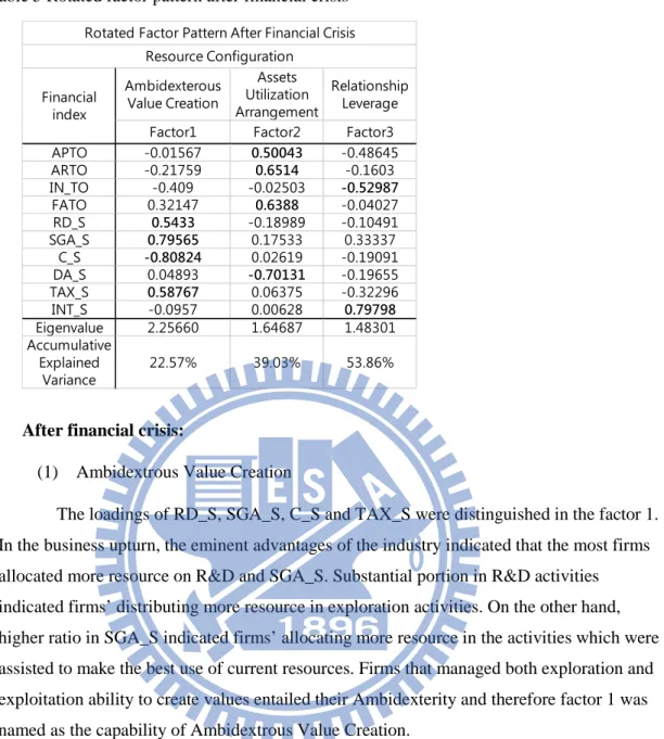
Table 5 Rotated factor pattern after financial crisis
After financial crisis:
(1) Ambidextrous Value Creation
The loadings of RD_S, SGA_S, C_S and TAX_S were distinguished in the factor 1. In the business upturn, the eminent advantages of the industry indicated that the most firms allocated more resource on R&D and SGA_S. Substantial portion in R&D activities indicated firms’ distributing more resource in exploration activities. On the other hand, higher ratio in SGA_S indicated firms’ allocating more resource in the activities which were assisted to make the best use of current resources. Firms that managed both exploration and exploitation ability to create values entailed their Ambidexterity and therefore factor 1 was named as the capability of Ambidextrous Value Creation.
The capability of Ambidextrous Value Creation was crucial to profit creation. The lower the C_S was, the higher the margin would be. In addition, Tax cost was one kind of inevitable byproducts of high margins. If the cost of SGA, RD, and TAX were high and C_S was lower, the capability of Ambidextrous Value Creation would be strong as well.
(2) Asset Utilization Arrangement
Factor 2 after financial crisis distinguished similar variables to those in factor 2 before financial crisis, which were APRO, ARTO, FATO and DA_S. Therefore, factors 2 here was also named as the capability of Assets Utilization Arrangement. However, of four variables in this period, DA_S and ARTO were more manifest than those in previous period. In other words, it suggested the firms placed more resource on managing sufficient and qualified production facilities in the economic upturn.
Ambidexterous Value Creation Assets Utilization Arrangement Relationship Leverage
Factor1 Factor2 Factor3
APTO -0.01567 0.50043 -0.48645 ARTO -0.21759 0.6514 -0.1603 IN_TO -0.409 -0.02503 -0.52987 FATO 0.32147 0.6388 -0.04027 RD_S 0.5433 -0.18989 -0.10491 SGA_S 0.79565 0.17533 0.33337 C_S -0.80824 0.02619 -0.19091 DA_S 0.04893 -0.70131 -0.19655 TAX_S 0.58767 0.06375 -0.32296 INT_S -0.0957 0.00628 0.79798 Eigenvalue 2.25660 1.64687 1.48301 Accumulative Explained Variance 22.57% 39.03% 53.86% Financial index Resource Configuration
Rotated Factor Pattern After Financial Crisis
(3) Relationship Leverage
INTO and INT_S were manifest among the variables in factor 3. The eminence of these two variables entailed the strong demand of cash flow. INT_S highlighted the
relationship with banks and creditors. Higher INT_S illustrated that the firms required more free cash flow from creditors at the cost of interests. If the INTO ratio was higher, it
indicated that the company managed inventory well and kept inventory in a reasonable level and it’s working capital was not sunk in the stock. One key factors of maintaining excellent management of inventory was the firm’s efficient and effective cooperation with suppliers. The efficiency and effectiveness were built from solid foundation such as mutually trust relationship.
Therefore, factor 3 was named as the capability of Relationship Leverage. If the score of factor 3 was higher and positive, it indicated the firm might perform poor logistic efficiency and bore higher interest burden. On the contrary if score was lower and negative, it indicated that firm enjoyed the benefits of the logistic efficiency and leveraged its strong relationship over suppliers.
4.3 Cluster analysis results
In order to avoid the multicollinearity issue, the research adopted the latent factors derived from previously PCA as new variables and ran cluster analysis independently for both periods. The research deployed two methods and Euclidean distance for the cluster analysis. Firstly the research ran several cluster analysis to compare the results of the clustering. According to rules of thumb to decide the better number of clusters, the larger CCC and Pseudo F statistic the better, the optimal cluster number for both two periods was inferred to be three in this research based on table 6.
Next, the wards method was applied to derive the centroid of each cluster. Wards method maximized the variance among groups but minimized the variance within groups. Therefore its centroids were most appropriate to be the seeds for K-means analysis. After assigning the seeds, the research followed up applying K-means method to calculate the Euclidean distance between each firm and seeds and to dispatch sample firms into different groups based on the distance.
Table 6 Criteria of optimal number of clusters
Below table presented the average scores of each factor of each cluster in two periods. The nomination for the clusters was determined on the features of each clusters. In order to picture out the underlying characteristics of the groups, the research also compared categorical information for each cluster and aimed to give an appropriate name for each cluster. The list of the subgroups was shown in appendix 1.
Table 7 Averaged factor scores in each cluster before crisis
Cluster Pseudo F A Rsquare CCC Cluster YEAR A Rsquare CCC
2 27.87 19.56 -6.29 2 43.20 25.75 -5.32
3 35.32 34.57 -6.26 3 47.76 45.47 -7.98
4 31.39 46.75 -10.62 4 51.03 61.41 -12.03
5 38.64 56.93 -10.60 5 45.27 67.09 -13.09
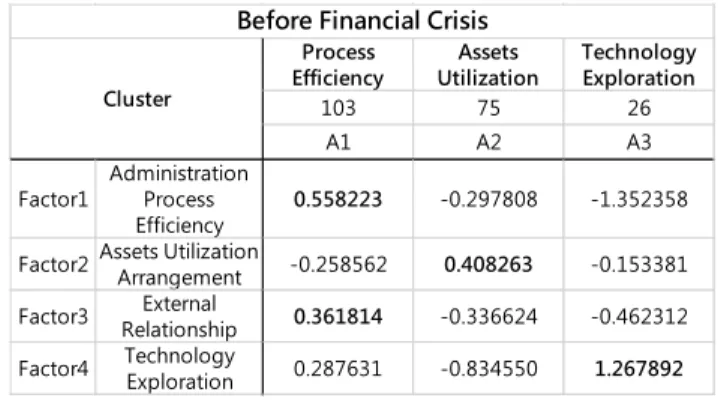
Before Financial Crisis After Financial Crisis Criteria of selecting optimal numbers of clusters
Process
Efficiency UtilizationAssets TechnologyExploration
103 75 26
A1 A2 A3
Factor1 AdministrationProcess
Efficiency 0.558223 -0.297808 -1.352358 Factor2Assets UtilizationArrangement -0.258562 0.408263 -0.153381 Factor3 RelationshipExternal 0.361814 -0.336624 -0.462312 Factor4 TechnologyExploration 0.287631 -0.834550 1.267892
Cluster
Before Financial Crisis
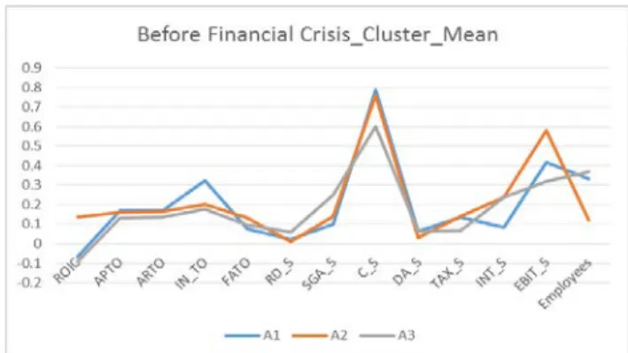
Figure 3 Comparison of factor scores mean among clusters before crisis
Before financial crisis:
(1) Cluster A1: Process Efficiency Group
More than half of the firms were classified into this group. The capability of managing Administration Process Efficiency and the capability of External relationship illustrated strong influence on the cluster. While further evaluating the variables mean of each cluster, it was found that this group had the highest C_S ratio but still maintained certain level of margins. The contrast indicated that there had some forces other than products helping the firms of the group to create margins. The higher Administration Process Efficiency factor scores projected that the group enjoyed the competitive advantage in managing administration process efficiency and prevented any unnecessary of resource wastes. However, in the economic downturn, the efficient advantage cannot guarantee positive ROIC. Even though the group preserved certain level of operation margin, its low margin was offset by the high portion of DA expenses and TAX costs.
(2) Cluster A2: Assets Utilization Group
The assets utilization group here was composed by smaller size of companies. The cluster showed strong capability of utilizing assets. The group was featured by the highest FATO rate, and lowest DA expense. Moreover, the group was the only cluster who
maintained the highest operation margins and enjoyed positive ROIC even in the economic downturn. The group had higher C_S but maintained most profitable margins. In sum, the group was currently harvesting its previous investment and hard efforts from the point of its lower DA_S ratio and R&D cost.
(3) Cluster A3: Technology Exploration Group
This group was classified according to its eminent capability of technology exploration. In figure 3, the group (A3) presented the highest SGA_S and RD_S among three groups, and the two high values indicated that the group was trying to balance resource in exploration and exploitation activities. This group was composed by the larger firms
among all 3 groups because its employee size was the largest. Its INT_S was remarkable high but TAX_S and the C_S was the lowest. The substantial investment in the RD and SGA seemed significantly offset the group’s profits because it had the lowest ROIC and EBIT_S.
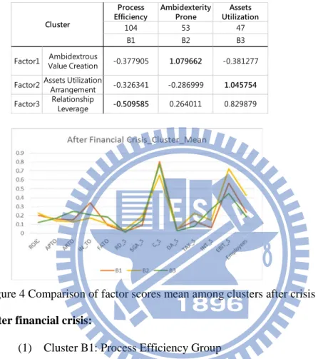
Table 8 Averaged factor scores in each cluster after crisis
Figure 4 Comparison of factor scores mean among clusters after crisis
After financial crisis:
(1) Cluster B1: Process Efficiency Group
Half of the firms was classified into this group which demonstrated competitive advantage in managing Process Efficiency. More than 80% of the members were notably overlapped with those was in cluster A1. Despite the group had the highest C_S, it had the lowest SGA cost and highest INTO rate. The group enjoyed a moderate ROIC rate. These data implied that the group managed lower product margin but they succeeded in exerting control over process efficiency to squeeze profits.
(2) Cluster B2: Ambidexterity Prone Group
This group was composed by large size firms and presented potential to generate the highest ROIC and profit margins, even though its administrative efficiency and asset
utilization were not salient among groups. The notable RD_S and SGA_S depicted the features of ambidextrous organizations. The group illustrated lowest C_S ratio and highest EBIT_S.
Process
Efficiency AmbidexterityProne UtilizationAssets
104 53 47
B1 B2 B3
Factor1 Value CreationAmbidextrous -0.377905 1.079662 -0.381277 Factor2 Assets UtilizationArrangement -0.326341 -0.286999 1.045754
Factor3 RelationshipLeverage -0.509585 0.264011 0.829879
Cluster
(3) Cluster B3: Assets Utilization Group
The assets utilization group here was composed by smaller size companies. The capability of Assets Management was standing out to feature the group. The group presented the highest FATO, ARTO and INT_S but the lowest RD_S, DA_S and TAX_S. Obviously, the group presented the poorer performance due to its lowest EBIT_S and ROIC. The group was inferred to enjoy the benefits of its previous investment due to its lowest DA_S ratio and high FATO ratio.
4.4 Discriminant analysis results
In order to verify the effectiveness of the cluster results, the research applied discriminant analysis to test the classification of clusters. The classification was further examine by hit ratio and cross validation hit ratio.
Before Financial Crisis
According to Table 9, total four factors showed statistically significance to
distinguish the clusters. The eigenvalues of the two canonical functions were larger than 1, which were 1.6734 and 1.167. The canonical correlation were larger than 0.6 and the accumulative explained variance was larger than 75%. Based on the rule of thumb, the two canonical functions were both tested statistically significant.
Table 9 Results of distriminant analysis before crisis.
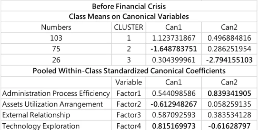
Table 10 revealed that the canonical function Can1 distinguished cluster 2(A2) from the others mainly according to assets utilization and technology exploration. Can2 was used to set apart cluster 3(A3) from others based on impacts of administration process efficiency and technology exploration.
Table 10 Results of discriminant canonical function before crisis
Factor1 1 0.762 0.7966 0.4251 0.7395 74.32 <.0001
Factor2 1 0.9542 0.3835 0.0985 0.1093 10.98 <.0001
Factor3 1 0.9343 0.45 0.1357 0.157 15.77 <.0001
Factor4 1 0.7069 0.8684 0.5052 1.021 102.61 <.0001
Statistic Value F Value Num DF Den DF Pr > F
Wilks'
Lambda 0.1726125 69.64 8 396 <.0001
Function CorrelationCanonical Eigenvalue Proportion Cumulative Pr > F 1 0.79117 1.6734 0.5891 0.5891 <.0001 2 0.733847 1.167 0.4109 1 <.0001 S=2 M=0.5 N=98 Discriminant Function Between Standard Deviation
Multivariate Statistics and F Approximations R-Square /
(1-RSq) Before Financial Crisis Univariate Test Statistics F Statistics, Num DF=2, Den DF=201
Variable R-Square F Value Pr > F Total Standard Deviation Pooled Standard Deviation
Numbers CLUSTER Can1 Can2 103 1 1.123731867 0.496884816
75 2 -1.648783751 0.286251954
26 3 0.304399961 -2.794155103
Variable Can1 Can2 Administration Process Efficiency Factor1 0.544098586 0.839341905
Assets Utilization Arrangement Factor2 -0.612948267 0.058259135 External Relationship Factor3 0.587092593 0.383534128 Technology Exploration Factor4 0.815169973 -0.61628797
Before Financial Crisis
Pooled Within-Class Standardized Canonical Coefficients Class Means on Canonical Variables
Moreover as shown in Table 11, among 103 firms in Process Efficiency Group, 99 firms were classified correctly; 69 of 75 firms in Assets Management Group were classified correctly; and 25 of 26 firms in Technology Exploration Groups were classified correctly. The overall hit ratio of prediction of the discriminant Analysis was up to 95.1% and hit ratio in cross validation was also up to 93.63%. In sum, these results of Discriminant Analysis supported the effectiveness of the clustering.
Table 11 Hit ratios of discriminant analysis and cross validation before crisis
After Financial Crisis
Table 12 illustrated that three factors were tested statistically significance to distinguish the clusters after financial crisis as well. The eigenvalues of canonical functions were 1.4225 and 0.8654. Both canonical correlations were larger than 0.6 and the
accumulative explained variance was larger than 75%. Although one of the canonical correlation was smaller than 1, the two canonical functions were tested statistically significant to distinguish clusters.
Table 12 Results of discriminant analysis after crisis
As shown in Table 13, Can1 set apart cluster 3 (B3) from the others according to assets utilization and relationship leverage. Can2 distinguished cluster 2 (B2) from others primarily based on the factor of ambidextrous value creation.
95.10% Cluster 1 2 3 Total A1 99 3 1 103 A2 3 70 2 75 A3 1 0 25 26 93.63% Cluster 1 2 3 Total A1 98 3 2 103 A2 4 69 2 75 A3 2 0 24 26 Predicted Classification Cross Validation
Before Financial Crisis
Factor1 1 0.7712 0.7834 0.4112 0.6983 70.17 <.0001
Factor2 1 0.823 0.7011 0.3293 0.4909 49.34 <.0001
Factor3 1 0.8344 0.681 0.3107 0.4507 45.3 <.0001
Statistic Value F Value Num DF Den DF Pr > F
Wilks'
Lambda 0.2212979 74.67 6 398 <.0001
Function CorrelationCanonical Eigenvalue Proportion Cumulative Pr > F 1 0.766287 1.4225 0.6217 0.6217 <.0001
2 0.681113 0.8654 0.3783 1 <.0001
Multivariate Statistics and F Approximations
S=2 M=0.5 N=98
Discriminant Function
After Financial Crisis Univariate Test Statistics F Statistics, Num DF=2, Den DF=201 Variable Total Standard Deviation Pooled Standard Deviation Between Standard Deviation
R-Square R-Square /(1-RSq) F Value Pr > F
Table 13 Results of discriminant canonical function after crisis
Table 14 revealed the hit ratio of the DA prediction: 98 of 104 firms in Process Efficiency Group were classified correctly; 50 of 53 firms in Ambidexterity Prone Group were classified correctly; 42 of 47 firms in Assets Utilization Groups were predicted finely. The overall hit ratio of predicted classification of the discriminant Analysis after financial crisis was up to 93.14% and hit ratio of cross validation was also up to 91.18%. These results noticeably supported the effectiveness of the clustering.
Table 14 Hit ratios of discriminant analysis and cross validation after crisis
Overall speaking, the hit ratios after financial was slightly lower than the rate before financial crisis. The decline implied that the firms’ resource configuration after crisis was not as distinguished as that before crisis. The firms were possibly trying different strategies for their future development.
Numbers CLUSTER Can1 Can2 103 1 -0.862422327 -0.606110293
75 2 -0.1689688 1.553022931
26 3 2.098878052 -0.410100953
Variable Can1 Can2 Ambidextrous Value Creation Factor1 -0.112294857 1.274626227
Assets Utilization Arrangement Factor2 1.132552094 -0.246440577 Relationship Leverage Factor3 1.050384278 0.40198694
After Financial Crisis Class Means on Canonical Variables
Pooled Within-Class Standardized Canonical Coefficients
93.14% Cluster 1 2 3 Total B1 98 2 4 104 B2 2 50 1 53 B3 1 4 42 47 91.18% Cluster 1 2 3 Total B1 96 3 5 104 B2 2 49 2 53 B3 1 5 41 47 Predicted Classification
After Financial Crisis
Cross Validation
4.5 Cross tabulation comparison for categorical variables 4.5.1 SIC
SIC was one kind of the classification code used to class by firms’ products or service. SIC 3711 included the companies whose products were classified in Motor Vehicles & Passenger Car Bodies and SIC 3714 represented the companies whose products were related to Motor Vehicle Parts & Accessories. Before crisis, about 95% of firms in 3711 were classified into Process Efficiency and Assets Utilization Group and only 3 companies were classified to Technology Exploration group, which were Honda, Volvo and BMW. After crisis, more firms was classified in to Ambidexterity Prone group in 3711 and 3714.
Table 15 Table of Cluster by SIC
4.5.2 Country
Of the firms analyzed in the research, 76 (37%) were Japanese companies, 32(15%) came from India, 21(10%) from the US and 13(6%) from Taiwan. Table 16 clearly revealed that over 80% of Japanese firms were classified into Process Efficiency Group in both periods. Over 60% of Indian companies were classed into Assets Utilization. The firms from the US were divided evenly in Process Efficiency and Assets Utilization groups in both periods. Taiwanese firms addressed the advantages in Process Efficiency before crisis, but after crisis half firms showed the advantages in Ambidexterity Prone. More than half of German firms were in Process Efficiency group before crisis but three 75% classified to Ambidexterity Prone group after crisis. The number of other countries was relative small and the comparison was not significant in the cross-table comparison.
Cluster SIC 3711 3714 Total Cluster SIC 3711 3714 Total
Process
Efficiency A1 (45.1%)23 (52.29%)80 (50%)103 EfficiencyProcess B1 (37.25%)19 (55.56%)85 (50%)104 Assets
Utilization A2 (49.02%)25 (32.68%)50 (36%)75 AmbidexterityProne B2 (21.57%)11 (27.45%)42 (25%)53 Technology
Exploration A3 (5.88%)3 (15.03%)23 (12%)26 UtilizationAssets B3 (41.18%)21 (16.99%)26 (23%)47 P-value
(0.0584*) Total (25%)51 (75%)153 (100%)204 (0.0017***)P-value Total (25%)51 (75%)153 (100%)204 Table of CLUSTER by SIC Before Table of CLUSTER by SIC after
Table 16 Table of Country by Cluster in two periods
4.5.3 Region
About 67% (137) of the firms in this analysis came from Asia, 19% (40) were from Europe and 11% (23) were from North America. About 60% of Asian were in were in Process Utilization group. Firms from North America preferred to apply strategy either Process Efficiency or Assets Utilization. European firms were divided into 3 groups evenly before crisis, but after crisis half were in Ambidexterity Prone group.
Table 17 Tables of Region by cluster
4.5.4 Employees
Employee number of a firm was used to address the firm size in the research. 56% of the companies were classified into large size firms whose employees were more than 3000 persons. Over 65% of the large firms were classified in Process Efficiency group in both periods. The large size indicated the importance of intensive capital and economic scales required in automobile and related industry.
Table 18 Table of cluster by Employee size
Cluster Country JPN IND USA TWN DEU Others Total Cluster Country JPN IND USA TWN DEU Others Total Process
Efficiency A1 (84%)64 (6%)2 (47%)10 (69%)9 (62%)5 (24%)13 (50%)103 EfficiencyProcess B1 (85%)65 (9%)3 (42%)9 (53%)7 (12%)1 (35%)19 (50%)104 Assets
Utilization A2 (10%)8 (87%)28 (42%)9 (7%)1 (0%)0 (53%)29 (36%)75 AmbidexterityProne B2 (10%)8 (31%)10 (14%)3 (46%)6 (75%)6 (37%)20 (25%)53 Opportunities
Exploration A3 (5%)4 (6%)2 (9%)2 (23%)3 (37%)3 (22%)12 (12%)26 UtilizationAssets B3 (3%)3 (59%)19 (42%)9 (0%)0 (12%)1 (27%)15 (23%)47 76
(37%)(15%)32 (10%)21 (6%)13 (3%)8 (26%)54 (100204 (37%)76 (15%)32 (10%)21 (6%)13 (3%)8 (26%)54 (100204
Total Total
Table of Country by CLUSTER Before Crisis Table of Country by CLUSTER After Crisis
Cluster REG AmericaNorth Europe Africa Oceania Asia Total Cluster REG AmericaNorth Europe Africa Oceania Asia Total Process
Efficiency A1 (47.83%)11 (30%)12 0 (0%) 0 (0%) (57.25%)79 (50%)102 EfficiencyProcess B1 (43.48%)10 (27.5%)11 0 (0%) 0 (0%) (59.42%)82 (50%)103 Assets
Utilization A2 (39.13%)9 (37.5%)15 (100%)1 (100%)1 (35.51%)49 (36%)75 AmbidexterityProne B2 (17.39%)4 (47.5%)19 0 (0%) (100%)1 (21.01%)29 (26%)53 Technology
Exploration A3 (13.04%)3 (32.5%)13 (0%)0 (0%)0 (7.25%)10 (12%)26 UtilizationAssets B3 (39.13%)9 (25%)10 (100%)1 0 (0%) (19.57%)27 (23%)47 P-value
(0.0027***) Total (11%)23 (19%)40 (0%)1 (0%)1 (67%)138 (100%)203 (0.0015***)P-value Total (11%)23 (19%)40 (0%)1 (0%)1 (67%)138 (100%)203 Table of CLUSTER by REGION Before Table of CLUSTER by REGION After
EMP personPer 0-500 3000500- 200003000- Total EMP personPer 0-500 3000500- 200003000- Total Process Efficiency A1 4 (33.33%) 23 (40.35%) 65 (73.03%) 92 (58%) Process Efficiency B1 5 (38.46%) 21 (42%) 64 (65.31%) 90 (55%) Assets
Utilization A2 (33.33%)4 (47.37%)27 (16.85%)15 (29%)46 AmbidexterityProne B2 (38.46%)5 (28%)14 (18.37%)18 (22%)37 Technology
Exploration A3 (33.33%)4 (12.28%)7 (10.11%)9 (12%)20 UtilizationAssets B3 (23.08%)3 (30%)15 (16.33%)16 (21%)34 P-value
(0.0001***) Total 12 (7%) 57 (36%) 89 (56%) (100%)158 (0.0448**)P-value Total 13 (8%) (31%)50 98 (60%) (100%)161 Table of EMP numbers by CLUSTER Before Table of EMP numbers by CLUSTER After
4.5.5 ROIC higher than average vs. ROIC lower than average
ROICD was a categorical variable defined to distinguish if the firm’s financial performance was better than industry average or not. Before financial crisis, the clusters didn’t reveal significant influence on the ROICD. However, after financial crisis, the differences among clusters proved significance in the 5% of confidence level. Of the group’s ROIC performance lower than industry, 50% were from Process Efficiency group after crisis, but the variation was not obvious in the higher ROIC group. It was referred that the competitive advantage of Process Efficiency could not guarantee stunning financial performance.
Table 19 Table of Cluster by ROICD
4.5.6 EBIT_S higher than average vs. EBIT_S lower than average
EBIT_SD was a categorical variables which divided the sample firms into two groups: either profit margin better than industry average or poorer. The division showed statistically significant differences among the clusters in both periods. In the poorer performance group, more than 60% of firms were from Process Efficiency group in both periods. In the group of higher than average, Assets Utilization group took almost 50% of the population before financial crisis, but after crisis Ambidexterity Prone group presented its critical role in the group.
Table 20 Table of EBIT_SD by clusters
Lower than average Higer than average Total Lower than average Higer than average Total Process Efficiency A1 37 (53.62%) 66 (48.89%) 103 (50.49%) Process Efficiency B1 65 (59.09%) 39 (41.49%) 104 (50.98%) Assets Utilization A2 20 (28.99%) 55 (40.74%) 75 (36.76%) Ambidexterity Prone B2 22 (20%) 31 (32.98%) 53 (25.98%) Technology Exploration A3 12 (17.39%) 14 (10.37%) 26 (12.75%) Assets Utilization B3 23 (20.91%) 24 (25.53%) 47 (23.04%) P-value (0.1584) Total 69 (33.82%) 135 (66.18%) 204 (100%) P-value (0.0328**) Total 110 (53.92%) 94 (46.08%) 204 (100%)
Table of CLUSTER by ROICD Before Table of CLUSTER by ROICD After
ROICD ROICD Lower than average Higer than average Total Lower than average Higer than average Total Process Efficiency A1 70 (61.4%) 33 (36.67%) 103 (50.49%) Process Efficiency B1 67 (63.81%) 37 (37.37%) 104 (50.98%) Assets
Utilization A2 (27.19%)31 (48.89%)44 (36.76%)75 AmbidexterityProne B2 (14.29%)15 (38.38%)38 (25.98%)53 Technology Exploration A3 13 (11.4%) 13 (14.44%) 26 (12.75%) Assets Utilization B3 23 (21.9%) 24 (24.24%) 47 (23.04%) P-value (0.0016***) Total 114 (55.88%) 90 (44.12%) 204 (100%) P-value (<.0001***) Total 105 (51.47%) 99 (48.53%) 204 (100%) Table of CLUSTER by EBIT_SD After
EBIT_SD EBIT_SD
Table of CLUSTER by EBIT_SD Before
4.5.7 Ambidexterity in R&D and SG&A
Ambidexterity (Amb_RS) variable here was defined as a firm’s RD_S and the SGA_S were both higher than 3-year average. On the other hand, a firm was classified into Not Ambidexterity if either one value was lower than industry average. In the analysis, both periods showed statistically significant difference among clusters.
Before crisis, of the Not ambidexterity group, most firms were divided evenly into both Process Efficiency group and Assets Utilization group. However in the period of after crisis, 60% of the firms were remarkably classified in Process Efficiency group.
Of the group defined to be with ambidexterity, half of the firms were from the Technology Exploration group before crisis, and yet 76% of the firms were from Ambidexterity Prone group after crisis.
Table 21 Table of AMB_RS by clusters
Not AMB With AMB Total Not AMB With AMB Total
Process
Efficiency A1 (53.85%)91 (34.29%)12 (50.49%)103 EfficiencyProcess B1 (57.87%)103 (3.85%)1 (50.98%)104 Assets
Utilization A2 (41.42%)70 (14.29%)5 (36.76%)75 AmbidexterityProne B2 (18.54%)33 (76.92%)20 (25.98%)53 Technology Exploration A3 8 (4.73%) 18 (51.43%) 26 (12.75%) Assets Utilization B3 42 (23.6%) 5 (19.23%) 47 (23.04%) P-value
(<.0001***) Total (82.84%)169 (17.16%)35 (100%)204 (<.0001***)P-value Total (87.25%)178 (12.75%)26 (100%)204
Table of CLUSTER by amb_rs Before Table of CLUSTER by amb_rs After
AMB_RS AMB_RS
4.6 ANOVA test on ROIC and EBIT rate among clusters
In order to examine if heterogeneous performance existed among clusters in each period, the research applied ANOVA test to examine ROIC and EBIT_S about each clusters. ROIC in the research referred to the overall return rate of the total investment of a firm. EBIT_S represented the pure margins of fundamental operation of a firm.
Below compared the financial performance between clusters in two periods. Before crisis, Asset Utilization group had the highest ROIC (1.34%) and EBIT_S (5.81%). After crisis, Ambidexterity Prone group had the highest ROIC (2.27%) and EBIT_S (8.54%).
Before crisis, Technology Exploration group had the lowest ROIC (-0.92%) and EBIT_S (3.2%). After crisis, Asset Utilization had the lowest ROIC (1.23%) and EBIT_S (4.45%).
The ANOVA results indicated that there was no statistically significant difference on ROIC1 among clusters for both periods. However, EBIT_S2 showed 85% statistically significance on the difference among clusters after crisis. While applying the Scheffe’s test to further examine the difference between groups, the EBIT_S of Ambidexterity Prone group (B2) showed statistically higher than Assets Utilization group (B3) in the analysis after financial crisis.
Table 22 ANVOA test of ROIC and EBIT_S
1 The normality test and Levene’s test didn’t support ROIC before crisis for the assumptions of normal
distribution of population and equality of variances among clusters. However, the normality test and Levene’s test supported ROIC after crisis for further ANOVA test, but its result was not statistically significant.
2 EBIT_S before crisis was not supported by Levene’s test for further ANOVA test. However in the
significant level of 15%, the Levene’s test for EBIT_S after crisis was statistically significant. While applying ANOVA test to EBIT_S after crisis, the result showed statistically significant. Therefore, the research degraded the significant level to 15% in ANOVA test.
1 2 3 1 2 3 Process
EfficiencyUtilizationAssets TechnologyExploration EfficiencyProcess AmbidexterityProne UtilizationAssets 103 75 26 104 53 47 Mean -0.0065 0.0134 -0.0092 Mean 0.0200 0.0227 0.0123 STD 0.0981 0.0336 0.0499 STD 0.0186 0.0234 0.0451 Mean 0.0417 0.0581 0.0320 Mean 0.0562 0.0724 0.0445 STD 0.0567 0.0638 0.0718 STD 0.0358 0.0854 0.0756 None Levene's
Test AnovaTest Scheffe's Test B2>B3* 0.1063 0.0775* <.0001*** 0.6114 <.0001*** 0.1541 0.9285 CLUSTER Nomality
Test Levene'sTest AnovaTest Numbers
0.0961* 0.6262 0.1691 ROIC
EBIT_S EBIT_S <.0001*** After Financial Crisis Before Financial Crisis
Scheffe's Test None None CLUSTER Nomality Test Numbers ROIC <.0001*** 26
4.7 Strategy transition
The research made a cross tabulation for the two classifications in two periods and resulted in 9 types of strategy transitions which represented possible swifts of competitive advantages in automobile industry. 83% (86/104) of the firms classified into Process Efficiency groups before crisis still remained in Process Efficiency Group after crisis. 83% (39/47) of the firms classified into Assets Utilization group before crisis still remained in Assets Utilization group after crisis. Of the firms classified into Ambidexterity Prone group after crisis, 41% (22 of 53) was from the Technology Exploration group and 38% (20 of 53) came from the Assets Utilization group before crisis.
The results implied that the majority of firms maintained the same type of
competitive advantages even went through the challenge of financial crisis. In other words, the competitive advantages derived in the research proved their reliability. In sum, the dominant competitive advantages of the automobile industry could be plausibly summarized into four types, which were Capability of managing Process Efficiency, Capability of maximizing Assets Utilization, Capability of insisting on Technology Exploration and Capability of maintaining Ambidexterity Prone.
The list of the firms in different types was shown in appendix 1.
Table 23 Cross Comparison of two clustering
Process Efficiency Ambidexterity Prone Assets Utilization B1 B2 B3 A1 Process Efficiency 86 (83%) 11 (21%) 6 (13%) 103 (50%) A2 UtilizationAssets 16 (15%) 20 (38%) 39 (83%) 75 (37%) A3 TechnologyExploration 2 (2%) 22 (41%) 2 (4%) 26 (13%) 104 (51%) 53 (26%) 47 (23%) 204 Table of Clusters Comparison before and after Financial Crisis Before
After
Total
Total
4.8 ANOVA test for 9 types of strategy transitions
The research applied ANOVA test to examine the financial performance of 9 types of groups from 2007 to 2012. The results indicated that there was statistically significant difference in ROIC3 at the confidence interval of 90%4.
Type 8 (A3B2), which was Technology Exploration then swift to Ambidexterity Prone, had the highest ROIC (6.18%) among all groups, and Type 2 (A1B2), which was Process Efficiency then swift to Ambidexterity Prone, had the highest EBIT_S (10.94%).
Type 6 (A2B3), which was classified into Asset Utilization in two periods, had the lowest ROIC (0.94%) and Type 7 (A3B1), which was Technology Exploration then swift to Process Efficiency, had the lowest EBIT_S (0.16%).
The research applied Scheffe’s test and further illustrated that ROIC of Type 8 (A3B2) was notable higher than ROIC of Type 1 (A1B1: Both periods were classified into Process Efficiency), Type 4 (A2B1: Asset Utilization swift to Process Efficiency), Type 5 (A2B2: Asset Utilization swift to Ambidexterity Prone) and Type 6 (A2B3: Both periods were classified into Asset Utilization).
Table 24 ANOVA test in ROIC & EBIT_S for 9 types of strategy transitions
3 Because the result of Levene’s test for EBIT_S didn’t support the assumption of equality of variances
among types, the research didn’t further discussed the ANOVA results of EBIT_S.
4 Because the result of Levene’s test for ROIC was statistically significant at confidence interval of 90%,
therefore, the research degraded the significant level to 10% in ANOVA test.
Test NomalityTest Levene'sTest AnovaTest
8>1*** 8>5*** 8>4*** 8>6*** EBIT_S <.0001*** 0.4439 0.0009*** None Mean Std Mean Std 1 A1B1 86 0.0223 0.0187 0.0455 0.0385 2 A1B2 11 0.0368 0.0136 0.1094 0.0778 3 A1B3 6 0.0367 0.0113 0.0158 0.0215 4 A2B1 16 0.0118 0.0095 0.0539 0.0335 5 A2B2 20 0.0169 0.0167 0.0850 0.0576 6 A2B3 39 0.0094 0.0091 0.0429 0.0686 7 A3B1 2 0.0599 0.0402 0.0016 0.0292 8 A3B2 22 0.0618 0.0552 0.0452 0.0779 9 A3B3 2 0.0347 0.0299 0.0937 0.0095
Difference in ROIC &EBIT_S for 9 types of groups Scheffe's Test ROIC <.0001*** 0.0793* <.0001*** A3B2>A1B1 A3B2>A2B2 A3B2>A2B1 A3B2>A2B3 None Mean and Std for 9 types of groups
G-ID G_type N ROIC EBIT_S
28