視訊品質控制之軟硬體協同設計與純粹硬體方法

全文

(1)國立交通大學資訊工程所碩士論文. 視訊品質控制之軟硬體協同設計與純粹硬體方法. Video Rate Control for Co-Design and Pure Hardware Approach. 研究生：陳京何指導教授：蔡淳仁教授. 中華民國九十三年六月. i.

(2) 視訊品質控制之軟硬體協同設計與純粹硬體方法 Video Rate Control for Co-Design and Pure Hardware Approach. 研究生：陳京何. Student：Ching-Ho Chen. 指導教授：蔡淳仁. Advisor：Chun-Jen Tsai. 國立交通大學資訊工程系碩士論文 A Thesis Submitted to Department of Computer Science and Information Engineering National Chiao Tung University in partial Fulfillment of the Requirements for the Degree of Master in Computer Science and Information Engineering June 2004 Hsinchu, Taiwan, Republic of China. 中華民國九十三年六月. ii.

(3) iii.

(4) 視訊品質控制之軟硬體協同設計與純粹硬體方法學生 : 陳京何. 指導教授 : 蔡淳仁. 國立交通大學資訊工程所碩士班. 摘要大部分軟體為主的視訊編碼器會在動作預測之後，對頻寬及失真作分析來確定量化器的大小，由動作預測單元得到的絕對誤差總和被使用來估計頻寬控制模式中的編碼複雜度。對於 SoC 平台上的視訊編碼器來說，如果要達到較佳的頻寬控制效能，由於需要計算複雜的數學模式，比較適合由微處理器來計算，而區塊編碼迴圈則是由 VLSI 加速器來執行。為了降低微處理器與加速電路溝通上的負荷，因此本論文設計出一套能在編碼迴圈外獨立執行的頻寬控制模式的方法。這個方法除了控制視訊編碼的資料流量之外，並可作場景變換偵測。另外，為了更進一步降低溝通上的負擔及簡化系統匯流排的設計，在此亦提出了查表方式的頻寬控制模式，用查表的方式取代複雜的碼率失真數學模型的計算，此演算法十分適合直接做在加速電路之中。總結而言，在此論文中，我們提出了一套適用於 SoC 平台上的視訊編碼器的迴圈外頻寬控制演算法，以及一個查表方式的頻寬控制演算法。由實驗結果可知，這些方法的效果極佳，很適合用在實際的系統中。. iv.

(5) Video Rate Control for Co-Design and Pure Hardware Approach Student : Ching-Ho Chen Advisor : Chun-Jen Tsai Department of Computer Science and Information Engineering Nation Chiao Tung University ABSTRACT Most software-based video encoders perform rate-distortion model analysis to determine the quantizer step size after motion estimation (ME). Typically, Sum of Absolute Differences (SAD) from the motion estimator is used as the complexity estimates for rate-control model. However, for video encoders on SoC platforms, the calculation of rate-control model is typically done on the microcontroller (MCU) core while the macroblock encoding loop (ME, transform, quantization, and entropy coding) is executed by ASIC accelerators. In order to reduce the communication overhead between the MCU and the ASIC accelerator, this thesis proposes a rate control algorithm that can be executed outside the encoding loop solely by the MCU is very useful. In addition, this thesis also proposes a lookup table approach that is suitable for pure hardware implementation. In this approach, the sophisticated R-D model is replaced with a lookup table and low complexity VLSI architecture can be used for rate-control for ASIC accelerators. Experimental results show that these algorithms are very promising for video codec hardware/software co-design and pure hardware implementation in practical systems.. v.

(6) Acknowledgement I am glad to finalize this thesis in favor of many people. First, my advisor, Chun-Jen Tsai, gives me much motivation and ideas, and encourages me to think in different viewpoints. Then, I also thanks for helps and comments from my seniors, juniors, and classmates. Of course, I want to thanks my family for giving me strong economic and moral support, especially for my dear mother. Finally, it is my pleasure to finish this thesis in my laboratory, MMES Lab of CSIE in NCTU.. vi.

(7) Content 1.. Introduction............................................................1. 1.1. Introduction to Rate Control ..............................................................................1 1.1.1. Buffer Issue ....................................................................................................1 1.1.2. Quality Variation............................................................................................1 1.1.3. Coding and Transmission Delay ....................................................................2 1.1.4. Granularity of Rate Control ...........................................................................2 1.1.5. Limitation of SoC Implementations...............................................................2 1.2. Video Encoder Architecture...............................................................................3 1.2.1. Introduction to Video Coding modules..........................................................4 1.2.2. Rate Control Illustration ................................................................................5 1.3. Research Motivation and Background...............................................................6 1.4. Problem Analysis ...............................................................................................8 1.4.1. Communication Overhead of Frame-Level Rate Control..............................8 1.4.2. Communication Overhead of Macroblock-Level Rate Control.....................8. 2.. Previous Work ......................................................10. 2.1. 2.2. 2.3. 2.4. 2.5. 2.6. 2.7.. Number of Encoding Passes for RC ................................................................10 Encoding Delay and RC...................................................................................10 Rate-Distortion Optimization and RC .............................................................10 Rate-Distortion Model for RC ......................................................................... 11 Frame Dependency .......................................................................................... 11 Variable Frame Rate RC ..................................................................................11 RC for SoC Platforms ......................................................................................11. 3.. Proposed RC Using Estimated Complexity.......12. 3.1. Rate control using a first order RD model .......................................................12 3.1.1. Frame Level Rate Control............................................................................12 3.1.2. Macroblock Level Rate Control...................................................................13 3.2. Out-of-Loop Video Rate Control for Software/Hardware co-Design..............17 3.2.1. Frame Complexity Estimation and Frame-Level Rate Control ...................17 3.2.2. Adaptive RD Model.....................................................................................18 3.2.3. Other Adaptive RD Model Methods ............................................................19 3.2.4. Macroblock Level Complexity Estimation and Rate Control......................20 3.3. Encoding of I-frames .......................................................................................23 vii.

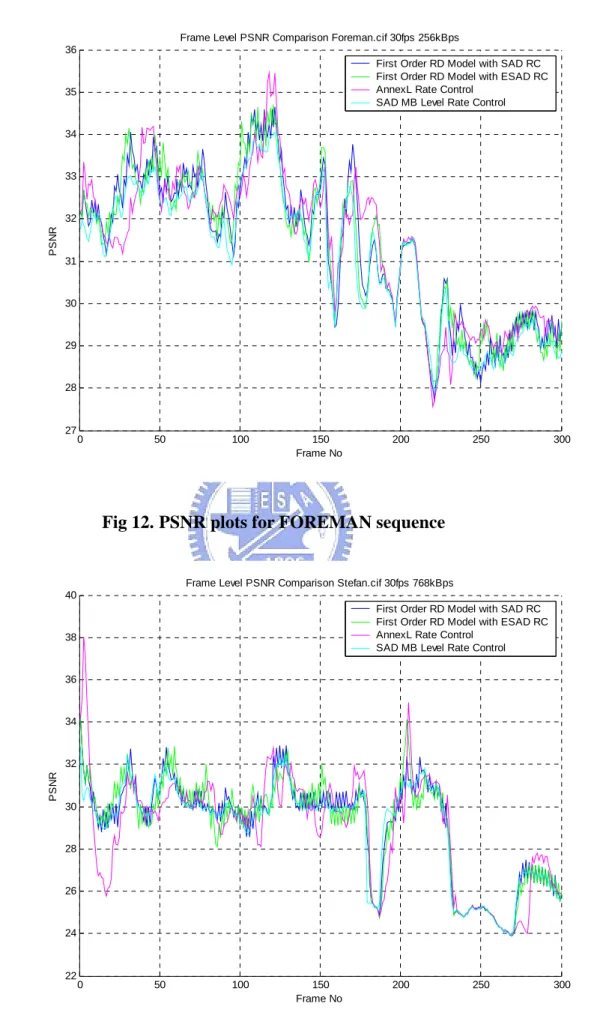
(8) 3.3.1. 3.3.2.. Scene Change Detection ..............................................................................23 Complexity Estimation for I frame ..............................................................24. 4.. Pure Hardware Rate Control..............................24. 4.1. 4.2. 4.2.1. 4.2.2. 4.2.3. 4.3. 4.4.. Consideration in Hardware Rate Control.........................................................25 Hardware Rate Control Approach....................................................................25 Process Flow of the H/W Rate Control Method ..........................................26 Modeling Table Indexing .............................................................................27 Update Modeling Table................................................................................28 Operations of the H/W Rate Control ...............................................................28 Hardware architecture of rate control ..............................................................30. 5.. Experiments and Analysis ...................................32. 5.1.. Testing Environment and Video Encoder Configuration.................................32. 5.1.1. Environment.................................................................................................32 5.1.2. Encoder Configuration.................................................................................32 5.2. Frame Level Rate Control Comparison ...........................................................33 5.2.1. PSNR............................................................................................................34 5.2.2. Frame Bits Variation ....................................................................................36 5.2.3. Buffer Status ................................................................................................38 5.3. Macroblock Level Rate Control Comparison ..................................................40 5.3.1. PSNR............................................................................................................40 5.3.2. Frame Bits Variation ....................................................................................43 5.3.3. Buffer Status ................................................................................................45 5.4. Comparisons Among Sequences......................................................................47 5.4.1. PSNR and Output Bitrate.............................................................................47 5.4.2. Mean and Standard Deviation for PSNR Variation .....................................48 5.4.3. Mean and Standard Deviation for Bits Variation .........................................50. 6.. Conclusion and Future Work .............................52. 6.1. Discussions ......................................................................................................52 6.2. Future Work .....................................................................................................52 6.2.1. Design Better Measure for Frame-Level or MB-Level Complexity ...........52 6.2.2. Use More Sophisticated R-D Model............................................................53. 7.. Reference ..............................................................53. viii.

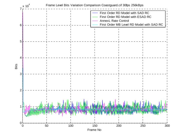
(9) Figure List Fig 1. Video Encoder Architecture ···············································································3 Fig 2. Rate Control Flow······························································································5 Fig 3. Data Flow Between MCU and ASIC Accelerator···············································7 Fig 4. Dual-Core SoC Platform Architecture································································7 Fig 5. MB Level Rate Control R-D Modeling····························································14 Fig 6. Communication Between MCU and Accelerator ·············································16 Fig 7. R-D Modeling for One Pack ············································································21 Fig 8. Modeling Table in Hardware Rate Control·······················································27 Fig 9. System Architecture of H/W Rate Control ·······················································31 Fig 10. Block Diagram of H/W Rate Control ·····························································31 Fig 11. PSNR plots for COASTGUARD sequence ····················································34 Fig 12. PSNR plots for FOREMAN sequence····························································35 Fig 13. PSNR plots for STEFAN sequence ································································36 Fig 14. Frame bits plots for COASTGUARD sequence ·············································36 Fig 15. Frame bits plots for FOREMAN sequence·····················································37 Fig 16. Frame bits plots for STEFAN sequence ·························································38 Fig 17. Buffer status plots for COASTGUARD sequence··········································38 Fig 18. Buffer status plots for FOREMAN sequence ·················································39 Fig 19. Buffer status plots for STEFAN sequence ······················································40 Fig 20. PSNR plots for COASTGUARD sequence····················································41 Fig 21. PSNR plots for FOREMAN sequence····························································41 Fig 22. PSNR plots for STEFAN sequence ································································42 Fig 23. Frame bits plots for COASTGUARD sequence ·············································43 Fig 24. Frame bits plots for FOREMAN sequence·····················································44 Fig 25. Frame bits plots for STEFAN sequence ·························································45 Fig 26. Buffer status plots for COASTGUARD sequence··········································45 Fig 27. Buffer status plots for FOREMAN sequence ·················································46 Fig 28. Buffer status plots for STEFAN sequence ······················································47. ix.

(10) Table List Tab 1. Tab 2. Tab 3. Tab 4. Tab 5. Tab 6. Tab 7.. Encoder Configuration ···············································································33 PSNR & Output Bitrate for Frame Level Rate Control ······························47 PSNR & Output Bitrate for Macroblock Level Rate Control······················48 Mean & Standard Deviation for PSNR Variation for Frame Level Rate Control ·······································································································49 Mean & Standard Deviation for PSNR Variation for Macroblock Level Rate Control ·······································································································49 Mean & Standard Deviation for Frame Bits Variation for Frame Level Rate Control ·······································································································50 Mean & Standard Deviation for Frame Bits Variation for Macroblock Level Rate Control ·······························································································51. x.

(11) 1. Introduction 1.1. Introduction to Rate Control Recently, digital video applications based on international standards (for example, H.263, MPEG-4 SP[1], and H.264 [2]) have become popular for embedded devices such as mobile phones, digital cameras, and PDAs. SoC platforms are commonly used to implement the core components of these devices. The most flexible and cost efficient way to realize a video codec on these platforms are to adopt hardware/software co-design. When applying digital video in different service environments, there are different transport/storage characteristics which should be taken into account in the encoding process. There are two types of video bitstreams, the first one is constant bitrate (CBR) bitstreams and the second one is variable bitrate (VBR) bitstreams. CBR traffics are preferred in most communication systems. However, compressed digital video is, by nature, composed of VBR data. This is due to the fact that complexity of video content varies across time, and it must be regularized by a rate control mechanism in order to achieve CBR. Unfortunately, enforcing CBR constraint reduces the quality of compressed video drastically, if not done properly. The encoder module that controls the data bandwidth of the video bitstream is called the rate-control (RC) module. While developing a suitable rate control mechanism, there are many important factors that have to be taken into account, such as, buffer usage and timing constraints, etc. These factors affect RC greatly and are discussed in the following subsections.. 1.1.1. Buffer Issue From rate-control point of view, the encoder must make sure that buffer overflow/underflow does not appear by controlling encoder buffer fullness during encoding process. As long as the decoder buffer is larger than or equal to the encoder buffer, there will be no buffer overflow/underflow problem. However, when unreliable transports between the encoders and the decoders are involved, the situation becomes much more complicated and is beyond the scope of this thesis.. 1.1.2. Quality Variation For block-based motion compensated video codec, the coded visual quality varies with the degree of motion. When the degree of motion in two consecutive frames is large and irregular, the performance of block-based prediction becomes worse. The error residuals in this case will be high and more bits are required to 1.

(12) encode the video data. In video encoding, the RC module controls the output bitrate by changing the quantization parameter, QP. Obviously, if constant quantization parameter (QP) is used for the whole sequence, the output bitrate will be VBR. If the RC module strictly enforces the CBR constraint, the video quality at high motion segments will be sacrificed. The fluctuation of visual quality in this case can be very large and are not tolerable by most viewers. The tradeoff between visual quality and output bitrate is the key to coding performance. In order to achieve good overall visual quality under a rate constraint, a good RC mechanism is needed.. 1.1.3. Coding and Transmission Delay For real-time applications such as videophone, videoconferencing, interactive system, etc., long delay for each compressed video frame is not permissible. In order to reduce the delay, both encoding delay and transmission delay must be reduced. Therefore, for such applications, the rate control module cannot apply sophisticated multiple-pass analysis or complicated prediction pattern such as B-frames.. 1.1.4. Granularity of Rate Control The granularity of rate control can be set at frame level or macroblock (MB) level. A frame-level rate control computes a single quantization parameter for each frame and applies buffer control to shape the overall output bitrate to match the target bitrate. A MB-level rate control method does not only set the quantization parameter for each frame but also adaptively changes the quantization parameter for each macroblock in a frame. Theoretically, the performance of MB-level rate controls should be better than frame-level rate controls. However, for MB-level rate control, it is not easy to fulfill rate constraint while maintaining constant quality. In addition, due to syntax limitation of MPEG-4 standard [1], the quantization parameter difference of two consecutive macroblocks must be less than or equal to 2. These difficulties make MB-level rate control more challenging.. 1.1.5. Limitation of SoC Implementations For a software-based rate-control, good coding efficiency can be achieved by employing sophisticated rate-distortion model for good quantization parameter selection. This is not suitable for a pure hardware implementation because it requires a powerful Arithmetic Logic Unit (ALU). On the other hand, a hardware/software co-design with rate-control algorithm embedded in the encoding loop would cause too much communication overhead between the MCU and the VLSI accelerator core. This overhead typically includes interrupts handling and excessive data transfer 2.

(13) overhead.. 1.2. Video Encoder Architecture. Source Picture. 1. Calculate Frame level Target bits. ME/MC. 2. Apply R-D Model Get QP. DCT. Quantize. 3. Adapt R-D Model. Reference Frame. IDCT. Inverse Quantize. ME: Motion Estimation MC: Motion Compensation QP: Quantization Parameter. MC. Fig 1. Video Encoder Architecture 3. VLC to Bitstrea.

(14) Fig 1 is the flow diagram for video encoder to generate the output bitstream. The blocks with solid lines are the essential processing elements and blocks with dashed lines are rate control points.. 1.2.1. Introduction to Video Coding modules In this section, we will give a brief introduction to the essential processing modules of a video encoder. The input video data to an encoder is usually in YCBCR format. In this representation, the luminance information (Y-channel, a.k.a. luma) is separated from the chrominance information (CB- and CR- channels, a.k.a. chroma). 1.2.1.1.. Motion Estimation/Motion Compensation. Each video frame is encoded using either inter-coding or intra-coding modes. Inter-coding modes (P-frame or B-frame) employs motion prediction to reduce the temporally correlated data while intra-coding mode (I-frame) operates directly on the pixel data of the current frame. For the first source frame, the only choice is intra-coding because there are no previous frames to support inter-coding. For subsequent frames, all three coding types (I, P, B frame) can be used. These coding modes also exist at the macroblock-level. However, some restrictions apply. For I-frames, only I-MBs are allowed. For P-frames, both I- and P-MBs are permissible. Finally, for B-frames, all coding modes are possible. The key to the performance of an video encoder is the mode decision algorithm (which can be part of the RC module) and the motion estimation algorithm. 1.2.1.2. DCT DCT is used to transform pixel data (I-MBs) or error residual data (P- and B-MBs) into frequency domain. 8x8 block size is used for the transform. That is, each MB is split into six 8x8 blocksfor the transform. 1.2.1.3.. Quantization. The quantization process reduces the entropy of the source data. This is the key technique to lossy coding. A properly-designed non-uniform quantizer can produce much better results than a uniform quantizer. However, for real-time video applications, uniform quantizer is often used. The RC module determines the quantization step size (QP) as a tradeoff between quality and distortion. 1.2.1.4.. IDCT and Inverse Quantization. In order to do predictive coding for the next frame, reconstructed frame should be stored in the reference frame buffer. Hence, there is a video decoder (minus the entropy decoder) embedded inside the encoder. Inverse quantization and IDCT are used to reconstruct spatial data from DCT coefficients which are different from the original coefficients due to quantization effect. 4.

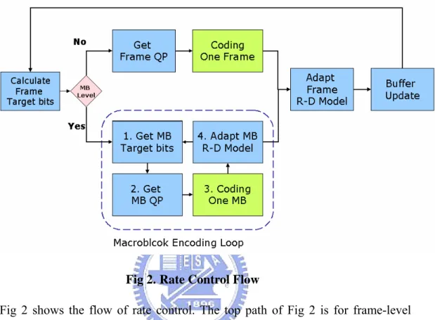
(15) 1.2.2. Rate Control Illustration In Fig 1, the blocks which are in dashed lines are an example of rate control points in a video encoder. As mentioned in previous section, there are two types of rate control, namely, frame-level RC and macroblock-level RC.. Fig 2. Rate Control Flow Fig 2 shows the flow of rate control. The top path of Fig 2 is for frame-level control, so the rate-distortion curve is modeled using entire frame; while the bottom path is macroblock-level control, which uses MBs as modeling units and adapts quantization parameters for each MBs. The main tasks for a typical rate control algorithm are described in the following sections. 1.2.2.1.. Calculate Frame Level Target Bits. The essential goal of rate control is to control the output bitrate, so the first task of RC is to compute the bit budget for current frame. Bit budget (a.k.a. bit-allocation) is obtained according to the status of buffer and possible pre-analysis for current frame content. In general, pre-analysis is employed to exploit the frame complexity and some critical information using the technique like image processing, probability modeling, and etc., and this may be one essential factor to improve the performance of rate control. It is important for RC algorithm to estimate the complexity of a frame/macroblock before the encoding loop starts so that the RC algorithm can controlled the quantization stepsize (QP) to meet the bit budget constraint. If QP is fixed, the more complex a frame/macroblock is the more bits it will take to encode. Since there is a strong correlation between the compressed data size and the 5.

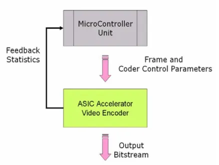
(16) sum-of-absolute-difference (SAD) of motion-compensated frame and current frame, consequently, SAD is often used to represent the degree of complexity. Good bit allocation algorithm could improve the overall visual quality, even if the same rate-distortion model is used. Therefore, this is a key differentiator among different video encoder implementations. 1.2.2.2.. Apply R-D model and Get QP. Given target number of bits (i.e. data rate), QP can be calculated from the rate-distortion model at macroblock-level or frame-level. Many algorithms approximate R-D curves with polynomial functions, logarithmic functions, or in a transformed domain (e.g. Rho-domain). Seleting a QP that fulfills the bit-budget constraint while maintaining consistent visual quality across macroblocks and video frames is one of the biggest challenges. 1.2.2.3.. Update R-D model. Because R-D model is content-dependent, a RC algorithm must adapt model parameters progressively during the encoding of a video sequence. After QP is determined and used to encode current frame, the actual bits used to code current frame could be obtained, and this information could help correct the R-D model parameters for next encoding iteration (for next frame or next macroblock). When scene change happens in a video sequence, the model parameters may need to be reset. A common practice is to encode the first frame at the scene change position as an I-frame and restart the RC modeling process from that point.. 1.3. Research Motivation and Background If hardware/software co-design approach is used to implement video encoder, a Microcontroller Unit (MCU) will take care of control flow, set the data path, and handles computation of complex mathematical model. An ASIC accelerator will be used to handle massive data processing (such as DCT/IDCT and motion estimation) to speed up the encoder. Fig 3 illustrates the data flow between MCU and ASIC accelerator. The shared data between the MCU and the ASIC may includes frame data and coder control parameters (such as the quantization parameters, QP’s). Typically, QP’s which will be calculated by the MCU and passed to the ASIC accelerator. However, the communication overhead may be expensive since it requires some information from the ASIC accelerator (in particular, the SAD values).. 6.

(17) Fig 3. Data Flow Between MCU and ASIC Accelerator Typically, encoder components in sold lines in Fig 1 are often integrated into the ASIC; while the components in dashed lines will be executed by the MCU. Fig 4 is a typical layout of the two cores and the shared memory device. This thesis tries to provide solutions to two different RC implementations. First, if hardware/software co-design approach is used, a out-of-loop RC algorithm is proposed to reduce the communication overhead between the MCU and the ASIC. Secondly, if pure-hardware RC is desired, a table-look up approach is proposed to simplify the hardware architecture while maintaining accurate modeling of complicated RD curves. Frame Memory. Data. Data. Addr. MCU. Data. Addr. Addr. Accelerator. Fig 4. Dual-Core SoC Platform Architecture. 7.

(18) 1.4. Problem Analysis Some analysis on the communication overhead for a hardware/software co-design codec framework is presented in this section. We assume that the ASIC is designed as a BUS master device and interrupt-driven communication between the MCU and the ASIC is used for the system.. 1.4.1. Communication Overhead of Frame-Level Rate Control Assuming a 50MHz ARM core and a 100MHz ASIC accelerator is used to encode a 30-Hz CIF resolution video sequence. Also assume that it takes 60 clock cycles to handles an interrupt and transferring SAD to MCU, and 30 clock cycles for the accelerator to get QP from the MCU. The communication overhead can be computed as follows.. Accelerator Waiting cycle = framerate * (clock cycles for interrupt and transfter SAD + clock cycles for accelerator to get QP ) = 30 * (60 + 30) = 2700 Accelerator usage of waiting MCU =. Accelerator waiting cycles 2700 = = 2.7 * 10 −3 % Accelerator total cycles 100 * 10 6. MCU interrupt cycles = framerate * clock cycyle for interrupt = 30 * 60 = 1800. MCU usage of interrupt =. MCU interrupt cycles 1800 = = 3.6 *10 −5 = 3.6 *10 −3 % 6 MCU total cycles 50 *10. 1.4.2. Communication Overhead of Macroblock-Level Rate Contr ol Accelerator Waiting cycle = framerate * (macroblocks per frame) * (clock cycles for interrupt and transfter SAD + clock cycles for accelerator to get QP ) = 30 * (22 *18) * (60 + 30) = 1069200 Accelerator usage of waiting MCU =. Accelerator waiting cycles 1069200 = = 1.0692% Accelerator total cycles 100 * 10 6. MCU interrupt cycles = framerate * (macroblocks per frame) * clock cycyle for interrupt = 30 * (22 *18) * 60 = 712800 MCU usage of interrupt =. MCU interrupt cycles 712800 = = 1.4256 *10 − 2 = 1.4256% 6 MCU total cycles 50 *10. According to the analyses above, while using macroblock-level rate control, the accelerator usage for waiting MCU is about 1.0692%, and MCU usage of interrupt is almost up to 1.42%. However, this is under the condition that MCU does not 8.

(19) execute any operations for rate control algorithm. The actual waiting cycles will be larger in real cases.. 9.

(20) 2. Previous Work Many rate control algorithms have been proposed for various scenarios. Depending on the applications, the policies should be targeted at fulfilling some constraints, such as buffer size, encoding delay, etc., mentioned in previous sections. Some of these published rate control algorithms are discussed in this chapter. The sections are classified based on the characteristics of the algorithms.. 2.1. Number of Encoding Passes for RC Some rate control methods encode each image block several times with different quantization parameters before it decides on the best parameter [4][6][10]. By multiple-pass encoding, the calculated rate-distortion models are more accurate and improves coding efficiency. On the other hand, the coding time and complexity increase a lot. Therefore, these methods are usually used for off-line encoding.. 2.2. Encoding Delay and RC In real-time communication systems, the end-to-end delay for transmitting video data needs to be very small, particularly in two-way interactive applications such as videophone or videoconferencing. Rate control designed for low-delay environment should take into account of delays for processing, buffering, and transmission [11][12]. To reduce the encoding delay, these techniques keep the complexity as modest as possible by using simple R-D model and low computational buffer control. To reduce transmission delay per frame (or over a small time window), the RC algorithms should avoid generating large frames at highly complex video scenes. In some applications, VBR rate control with low delay ability could be use for real-time encoding for the purpose of digital storage [21].. 2.3. Rate-Distortion Optimization and RC The goal of rate-distortion optimization (RDO) is to achieve best quality-distortion tradeoff by selecting proper encoding modes and motion vectors. Although RDO can be used independently to the RC module, optimal results only achieved when both algorithms are designed jointly. Some rate control mechanisms employ Lagrangian optimization techniques [4][5][17] to exploit the better control parameters. Typically, these methods measure the rate-distortion characteristics and perform pre-analysis on future frames. Some methods apply dynamic programming to get the optimal control point by using previous/future frame information [3]. In 10.

(21) general, more memory and computation are required for this kind of approaches.. 2.4. Rate-Distortion Model for RC In order to estimate correct rate and distortion control points, different types of R-D models are proposed. Among these models, some are based on the modified version of the classical R-D functions which uses logarithmic expressions [11]. Other types of models use power functions [6] and polynomial functions [8]. These R-D models try to estimate the correct behaviors under some criteria such as bitrate, delay, etc. Traditionally, the distortion is specified in QP domain. Recently, a new R-D function in different domain is proposed for rate-distortion analysis [18]. By transforming the R-D function to a different domain, it can be shown that better quantization parameters can be obtained to satisfy given rate constraint.. 2.5. Frame Dependency Video coding removes large redundancy by using predictive coding, in which a given frame is dependent on previous and/or future frames. Good rate control algorithms should take prediction types into account to achieve better results [10][11][12]. For example, increasing the bits for a P frame would decrease the distortion in that P frame and, equivalently, increase its PSNR. This would likely increase the PSNR of the B frames which predicted from this P frame as well. Equivalently, I frames also could have the same effect on other frames.. 2.6. Variable Frame Rate RC To enhance coding efficiency, some rate control algorithms using variable frame rate to achieve good balance between spatial and temporal quality [17][20]. However, variable frame rate would introduce flickering and motion jerkiness, which degrade video smoothness. Some methods are also presented to reduce flickering effects by finding good tradeoff in both spatial and temporal quality.. 2.7. RC for SoC Platforms On SoC platofmrs, both available computational power and memory bandwidth are limited. Some rate control methods are proposed for SoC platforms [19] with lower requirements on memory bandwidth. In order to improve the performance on SoC platforms, this thesis proposes an algorithm for hardware/software co-design implementation and another algorithm for pure VLSI implementation. The experiments show promising performance compared to other more complex rate control methods for more powerful platforms. 11.

(22) 3. Proposed RC Using Estimated Complexity The proposed method is based on the first order Rate-Distortion (RD) model [15], in which Q ⋅ R λ = X , where Q is QP, R is bit, X is complexity and λ=1,. (1). to estimate the quantization step size used in next encoding. A typical rate-control algorithm uses the SAD of current frame (or previous macroblocks) computed by the motion estimator as a complexity measure in order to estimate the quantization step sizes. Even though more complex RD model has been proposed described in previous chapter, it is not suitable for hardware implementation. To facilitate hardware/software co-design implementation, the quantization step size must be estimated before entering the macroblock encoding loop. The rationale here is to reduce the amount of interaction between the MCU core and the dedicated multimedia ASIC. In this section, an algorithm is proposed to estimate the complexity of current frame using statistic information.. 3.1. Rate control using a first order RD model The expression of proposed rate control could be reformatted as following first order RD model based on Eq (1),. R =α ⋅. C Q. (2). ,where R is the frame size (in bits), C is the complexity of the frame, and Q is quantization step size (QP) which controls distortion. The scaling factor α is a parameter that adjusts the RD model to fit different types of video contents. It is important to note that α is not time-invariant. It can vary from one frame to the next. However, in this section, we assume that α is a constant throughout the video sequence.. 3.1.1. Frame Level Rate Control If R, C, and Q for the previous frame and R and C for the target frame are available, two equations could be established:. 12.

(23) α ⋅ C t arg et = Rt arg et ⋅ Qt arg et , (3). α ⋅ C prev = R prev ⋅ Q prev . Hence, the following equation can be used to compute the current quantization step size Qtarget (namely, QP):. Qt arg et =. C t arg et ⋅ R prev ⋅ Q prev C prev ⋅ Rt arg et. (4). Typically, R stands for the size of the frame (in bits), C is estimated from SAD for motion-compensated P frames and the sum of pixel deviation for intra-coded I frames, and Q is measured by the quantization step size QP. Large QP implies high distortion. Even though this is a very simple RD model, it is shown later that the model performs very well against more sophisticated models. In order to avoid bitrate fluctuation, the target size of the frame, Rtarget, is computed using a sliding window of N frames based on the target bitrate B and the target frame rate F. In addition, efficient buffer utilization is preferred, so it is necessary to maintain the buffer utilization at some specific percent of buffer usage, ω, (i.e. 0<ω<1). The average target frame size can be calculated as B/F, and the initial video decoder buffer size is V0 = (N × B/F) × (1 –ω). If previously coded frame is K bits, and the available video decoder buffer size is V then the updated available decoder buffer size is V ’= (V – K) + B/F. For the next frame, the target frame size is Ptarget = V ’+ B/F – V0 for a P-frame. Since the average I frame size is about three or four times bigger than a P frame ([16], Annex-L), the target frame size for I frame is k × Ptarget (k = 4~9, depending on the characteristics of the video sequence). The rate control algorithm must compute QP using Eq (4). Before the encoder enters the macroblock coding loop, the only term that is missing from Eq (4) is the target frame complexity estimate Ctarget.. 3.1.2. Macroblock Level Rate Control If the MB level rate control scheme is adopted, each QP of MB should be calculated. By considering two sets of MBs, non-coded and coded MBs, the two equations are established:. 13.

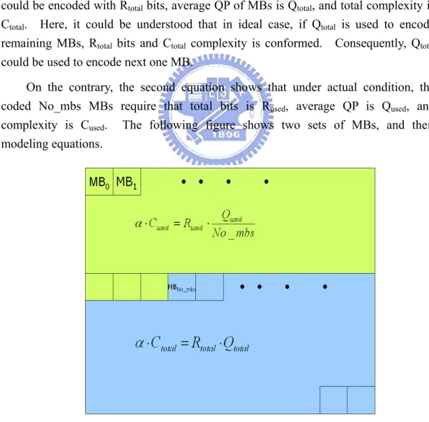
(24) α ⋅ Ctotal = Rtotal ⋅ Qtotal , α ⋅ C used = Rused. Qused , ⋅ No _ mbs. (5). in which Ctotal is total complexity (SAD for inter MB and deviation for intra MB) in remaining MBs, Cused is the complexity of coded MBs, Rtotal is the number of bits which could be used to encode remaining MBs in current frame, Rused is the number of bits used to encode previous MBs, Qtotal is the average QP of remaining MBs, Qused is sum of QPs of previous MBs, No_mbs is the number of encoded MBs, and Qused/No_mbs is average QP of coded MBs. In Eq (5), the first equation shows that under ideal condition, the remaining MBs could be encoded with Rtotal bits, average QP of MBs is Qtotal, and total complexity is Ctotal. Here, it could be understood that in ideal case, if Qtotal is used to encode remaining MBs, Rtotal bits and Ctotal complexity is conformed. Consequently, Qtotal could be used to encode next one MB. On the contrary, the second equation shows that under actual condition, the coded No_mbs MBs require that total bits is Rused, average QP is Qused, and complexity is Cused. The following figure shows two sets of MBs, and their modeling equations.. Fig 5. MB Level Rate Control R-D Modeling. 14.

(25) In terms of previous two equations, the QP of next MB could be obtained. Qmb = Qtotal =. C total ⋅ Rused Qused ⋅ . C used ⋅ Rtotal No _ mbs. (6). After encoding current MB, the variables in Eq (6) should be updated to maintain the correctness of coding status. 3.1.2.1.. Initialization. The initialization of frame level information is the same as what is described in previous section. After applying the frame level mechanism to get QP and available bits for current frame, the QP could be used to encode the first MB. Initially, Ctotal and Rtotal are set to frame complexity Ctarget and target frame bits Rtarget in Eq (4), respectively. Also Cused, Qused, Rused, and No_mbs are set to zeros. 3.1.2.2.. Get QP for current MB. Use Eq (6) to acquire the QP for current MB and encode current MB. Because of the limitation in standard bitstream syntax such that the different of QPs in current and previous MBs could not exceed +/-2 and some MB modes (i.e. NOT_CODED and INTER4V) could not change its QP, the QP for current MB should be well-managed to take care of these conditions. 3.1.2.3.. Update MB level information. After encoding current MB, update the variables in Eq (6) by using following equations: C total = C total − MB _ SAD , Rtotal = Rtotal − MB _ Bits , C used = C used + MB _ SAD , (7). Rused = Rused + MB _ Bits , Qused = Qused + Qmb ,. No _ mbs = No _ mbs + 1 , in which MB_Bits is the actual number of bits for coding this MB, MB_SAD is 15.

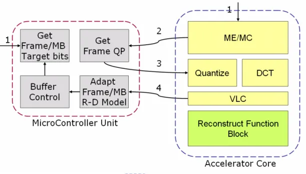
(26) the complexity measured in SAD for inter MB and deviation for intra MB. After updating variables, if there is any MB to be encoded, go back to section 3.1.2.2. 3.1.2.4.. Update frame level information. After all MBs in current frame are encoded, use the same way as frame level in section 3.1.1 to update frame parameters and buffer status for estimating the QP of next frame. Then, continue to encode next frame by repeating steps above. Most software-based encoder computes the complexity estimates after motion estimation for P frame since SAD are closely related to the complexity of a motion compensated frame.. Fig 6. Communication Between MCU and Accelerator. Fig 6 explains the communications between MCU and accelerator. The numbers marked in figure shows the execution order, and the same number means that they could be processed in parallel. In step 2, the SAD for current frame/MB is transferred to MCU and applies R-D model to get QP. After MCU gets QP for frame/MB, QP is transferred back to accelerator in step 3. Then, accelerator continues to quantize blocks and do variable length coding. In step 4, accelerator sends the coding bits and QP for coded frame/MB to MCU to adapt the Frame/MB R-D model. If frame level rate control is adopted, this needs one time to execute 4 steps above and might not be very critical. If macroblock level rate control algorithm is employed, these steps will be repeated as many times as total number of MBs in one frame. The performance would degrade strictly while MCU is busy in jobs. However, in order to simplify hardware design for a VLSI codec implementation, the proposed algorithm estimates the complexity without resorting to the motion 16.

(27) estimator.. 3.2. Out-of-Loop Video Rate Control for Software/Hardware co-Design Motion estimation exploits the correlated information between the reference frame and the target frame and greatly reduces the redundancies of the source data. The coding cost (complexity) of a target frame is measured by the total energy of the motion-compensated error residuals. However, motion estimation requires a lot of computational complexity and memory bandwidth that it is often done in ASIC. On the other hand, rate control requires many computations based on a RD mathematical model that the task is more suitable for a microcontroller (MCU). Therefore, it would be useful if the coding complexity can be estimated outside the motion estimator, either by the MCU or the video preprocessor that is common to most real-time video capturing systems.. 3.2.1. Frame Complexity Estimation and Frame-Level Rate Contr ol In this section a low complexity algorithm for the estimation of Ctarget is proposed to facilitate SoC based video codec implementations. The estimation is based on the statistics of image pixel differences of the reference frame and the target frame. The algorithm is listed as follows: z. Compute the frame difference between the current frame and the reference frame, scanline by scanline. If necessary, this process can be done on the subsampled frames to reduce memory bandwidth.. z. For each N×M region, R, of the difference image, compute its deviation and mean: mean(R ) =. 1 NM. ∑ luma _ diff i∈R. i. ,. deviation(R ) = ∑ abs (luma _ diff i − mean ) , i∈R. where luma_diffi is the component value of the luma channel difference image at pixel i. Again, if memory access is of concern, N can be set to 1 so that the procedure is done on a scanline basis. 17.

(28) z. Compute the estimated complexity χ for the target frame:. χ=. ∑ mean(R ) ⋅ deviation(R ). (8). R∈ frame. z. At this point, χ describes the complexity of the frame, but it is not in the same scale (unit) as SAD. We must adjust the scale of χ to match the scale of SAD for the RC algorithm to work. A simple linear scaling factor (a/b) is applied here to do the job: ˆ C target = a ⋅ χ / b. Note that in order to simplify hardware implementations, the parameter a is an integer and b is an integer power of two (b can be fixed to, say, 216). That is, the division can be implemented using right shift. z. After encoding of each frame, refine the parameter a by the following equation:. a = b ⋅ SAD target / χ ,. where SADtarget is the true motion compensated SAD value of the target frame. Note that scene change detection can be achieved using χ as well. If χ is larger than certain threshold, then the target frame should be encoded as an I-frame. In the following section, experiments have been conducted to determine this threshold.. 3.2.2. Adaptive RD Model In the first order RD model (Eq. (2)), the parameter, α, is assumed to be stationary, namely, it stays the same throughout the whole sequence. However, in most cases, α is content dependent and varies along the video sequence. In order to adopt an adaptive first order RD model, a new parameter, β, is introduced as follows,. Qt arg et = β ⋅. C t arg et ⋅ R prev ⋅ Q prev C prev ⋅ Rt arg et. .. (9). 18.

(29) In Eq (9), β is equivalent to αtarget/αprev, where αtarget and αprev are the RD model parameters for the target frame and the previous frame, respectively. After the encoding of one frame, β can be recalculated using Eq (10):. β=. C prev ⋅ Rt arg et ⋅ Qt arg et. (10). C t arg et ⋅ R prev ⋅ Q prev. The parameter β can be computed using a moving average window, that is, by averaging variable of β for each frame in the window. The adaptive RD model (Eq.(9)) is obtained using the relation of two consequent frames. It is possible to use other adaptive RD models here. If a fixed RD model is used, then α can be computed at any frame by the following equation:. α=. Rt arg et ⋅ Qt arg et C t arg et. .. The difference between the fixed RD model and the adaptive model is that in general for low frame rate cases the adaptive model has lower bit variation, while in high frame rate cases the fixed RD model has lower bit variation. This is because that in low frame rate cases, the motion between frames dominates the complexity and the adaptive model utilizes the relation between frames to have a better prediction of QP. With the frame rate becoming higher, the amount of motion decreases, and sometimes the “noise” (unpredictable part of the content) dominates the complexity.. 3.2.3. Other Adaptive RD Model Methods Based on the same RD model, one of some factors affecting the visual quality is how to adapt the RD model, how well this is managed is corresponding to how efficient the encoder is. Moreover, each adaptive strategy will result in different characteristic, such as bitrate variation, PSNR variation, decoder buffer usage, and etc. According to the situation and limitation, some adaptive RD model could be design for specific domain and application. Here in order to reduce the complication in MCU, the adaptive RD model method is as dedicated as possible. In addition to the adaptive method in the proposed rate control, moving average window, some other adaptive methods could be under consideration. Historical Weighted:. 19.

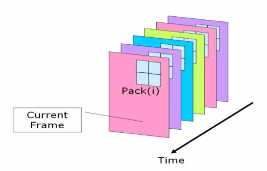
(30) β ' = β history ⋅ (1 − weight ) + β now ⋅ weight where βnow is the parameter calculated for current frame, βhistory is the history for β, and weight is used to adjust the proportion between βhistory and βnow. Outlier Removal: z. Respectively take the average of R, C, Q , and get the model parameter, β,in a moving average window. z. Use the model parameter, β, to compute standard error as threshold, and remove the data point which error is over the threshold. z. Recalculate the model parameter β after removing outlier point. Above these are some direct points of view to solve the adaptation problem of RD model, some RD models using other aspects to treat this trade-off matter, like variable encoding frame rate [17], rho-doman [18], and etc. Although in most advanced adaptable RD models could have good performance and coding efficiency, they are often used in software implementation and not introduced in hardware-based system due to complicated calculation.. 3.2.4. Macroblock Level Complexity Estimation and Rate Control If the macroblock level rate control is employed, the MB level approach in section 3.1.2 could not be used directly even though the macroblock complexity could be estimated by introducing the algorithm in section 3.2.1. Because each QP of MB should be acquired before entering MB encoding loop, there is no information about number of bits used for previous coded MBs. For example, if QP of the 10th MB would be computed using Eq. (6), because the number of bits used to encode previous 9 MBs could not be obtained before entering encoding loop, the formula cannot be applied. Consequently, a novel algorithm is proposed to take care of this issue. 3.2.4.1.. Rate-Distortion Modeling. Because each MB QP is needed before the encoding is started, the only information which could be obtained is the results of previous encoded frames, and the rate-distortion relation of MB can use the way like frame level to model. In order to exploit correlation between rate and distortion for each MB, the specific modeling unit, pack, which includes U MBs (i.e. 1 ≤ U ≤ total number of MBs in frame), is chosen.. 20.

(31) Fig 7. R-D Modeling for One Pack. Fig 7 above shows one 4-MBs pack, and the co-located packs in previous frames are used in R-D modeling. Certainly, the pack are not limited in the shape of square, it could be arranged in rectangle or any other shape of MBs according to the image content. Based on the first order R-D model, each pack in current frame could apply following formula to get its QP:. Qcur _ pack =. C cur _ pack ⋅ R pack. ⋅. Q pack. C pack ⋅ Rcur _ pack No _ mbs. ,. (11). where Ccur_pack is the complexity for current pack, Cpack is the complexity of previous frame measured by SAD, Rcur_pack and Rpack are the target bits for current pack and coded bits for previous pack, respectively. Qpack is the sum of QPs for previous frame and No_mbs is the number of MBs in pack. Equally, the only term missed in Eq. (11) is the Ccur_pack, and this could be estimated using proposed algorithm. In this way, all QPs of MBs in current pack could be given as the same value, Qcur_pack. Obviously, choosing adequate size of pack is a critical consideration for accurate and stable modeling. 3.2.4.2.. Macroblock Complexity Estimation. In order to get QP for each macroblock using Eq. (11), the complexity of each pack could be estimated using following procedure which is similar to estimation for frame complexity: 21.

(32) z. Compute the frame difference between the current frame and the reference frame. If necessary, this process can be done on the subsampled frames to reduce memory bandwidth.. z. For each N×M region, R, of the difference image, compute its deviation and mean: mean(R ) =. 1 NM. ∑ luma _ diff i∈R. i. ,. deviation(R ) = ∑ abs (luma _ diff i − mean ) , i∈R. where luma_diffi is the component value of the luma channel difference image at pixel i. Because the complexity of each pack comes from each region in each pack, the size of N×M should choose suitable value. z. Compute the estimated complexity χpack(i) for the each pack:. χ pack (i ) =. z. ∑ mean(R ) ⋅ deviation(R ). R∈ pack (i ). (12). χpack(i) describes the complexity of the i-th pack, but it is not in the same scale (unit) as SAD. We must adjust the scale of χpack(i) to match the scale of SAD for the RC algorithm to work. The same linear scaling factor is applied here to do this:. ˆ C pack (i ) = a pack (i ) ⋅ χ pack (i ) b. z. After encoding of each frame, refine the parameter apack(i) by the following equation: a pack (i ) = b ⋅ SAD pack (i ) χ pack (i ) ,. where SADpack(i) is the true motion compensated SAD value of the i-th pack. Note that scene change detection can be achieved using sum of all 22.

(33) χpack(i) as well.. The bus overhead savings of this approach, compared with conventional rate-control, are quite large. First of all, there is no lock-step synchronization (at macroblock level in the worse cases) between the MCU and the accelerator core. Lock-step synchronization between two cores is typically achieved via either interrupts or semaphores which are very inefficient for high speed SoC implementation due to loss of parallelism. Secondly, the proposed approach does not require passing of the SAD data (per macroblock) from the accelerator to the MCU over internal bus after each one macroblock is encoded which also saves memory bandwidth and time for bus arbitration. Because parameters of the R-D model and complexity estimation need to be updated, one interrupt and data transfer for entire frame information are required, and this don’t need much time compared to interrupt in encoding loop. Even though only one interrupt per frame is needed, the communication between MCU and the accelerator core is still one cost. If this time could be removed and no communication is need, all the work could be accomplished in the accelerator core. Therefore, one novel pure hardware rate control is proposed in next chapter and the issues described in section 1.3 should also be considered.. 3.3. Encoding of I-frames 3.3.1. Scene Change Detection When scene change happens, the current frame can not be predicted effectively from the previous frame. In this case, forcing the current frame to be encoded as a P-frame requires more bits. It is better to encode a scene change frame as an I-frame since the coding efficiency could be higher. Furthermore, I frames are independently decodable and therefore are more robust than P-frames. The technique proposed in section 3.2.1 for P-frame coding complexity estimation can be applied to scene change detection as well. If the complexity of a P-frame is too high, it is better off to encode it as an I-frame. In other words, if χ in Eq. (8) is larger than certain threshold, the target frame should be treated as a scene change frame. In addition, in order to avoid too many I-frames for low frame rate sequences and for long scene transitions, a constraint is set to enforce a minimal distances between I-frames. The minimal I-frame distance is determined based on the magnitude of the value χ.. 23.

(34) 3.3.2. Complexity Estimation for I frame Before encoding the scene change frame as an I-frame, the quantization step size for I-frame should be determined as well. However, quantization step size can not be computed using the same RD model as that for the P-frame. Because the P frame is motion-compensated while the I-frame is intra-coded, they are different intrinsically coding methods. A different RD model for I-frames is used here. It is also based on the first order RD model (Eq. (2)). By using equation Eq. (4), the quantization step size for I-frame is computed with Ctarget estimated as follows. To computing the Ctarget for an I-frame, the statistics (mean and deviation) are obtained from the luma intensity directly. The algorithm is listed as follows: z. For each N×M region, R, of the target frame, compute its mean and deviation using luma intensity.. z. Compute the estimated complexity χ for the target frame as the same as Eq. (8). z. Adjust the scale of χ to match the scale of SAD for the RC algorithm to work. Here a simple linear factor is also used as before and it introduced another factor, Ia to distinguish from the scale factor for P-frame: ˆ C target = I a ⋅ χ / b. Again, a power of two is selected for b. The initial value for Ia and b can be determined by using a two-pass encoding of the very first frame. z. After encoding the target frame as one I frame, Ia should be refined according to true encoded frame size. '. I a = I a ⋅ Rt arg et / Rtrue. where Rtrue is the true frame size encoded using Dtarget.. 4. Pure Hardware Rate Control Due to the preferred flexibility of rate control approach and to simplify design in the accelerator core, the rate control algorithm is implemented in the way of 24.

(35) software/hardware co-design, which is emphasized in section 3. By using this kind of co-design rate control, the performance of entire system could be promoted and use less time to encode video sequence. Because the time and memory bandwidth used to communicate between MCU and the accelerator core is primary bottleneck, it must be managed more elegant to remedy. In order to reduce the cost of system bus bandwidth and interrupt overhead to the microcontroller for the bit rate update and assignment to each MB, it’s suitable to implement a hardware rate control mechanism instead of utilizing the MCU. A hardware rate control implementation inside the MB encoding loop of the accelerator ASIC greatly reduces the number of data transfer and interrupt overhead between the MCU and the ASIC [19].. 4.1. Consideration in Hardware Rate Control The reason why rate control is preferred being implemented using software is the complicated mathematic model will do harm to hardware design and result in inflexibility and larger cost. In order to implement rate control in hardware, the complex mathematic analysis and lots of memory space must be reduced, and reformatted to be adopted in logic design. In addition, in view point of hardware, the difference of the clock cycles between addition and multiplication are large, so the more multiplication or division operations, the slower the accelerator core is. Hence when designing a rate control algorithm suitable hardware implementation, it is important to introduce simple operations to model rate distortion behavior. Within this limitation, the R-D model which only uses simple mathematic operations could not work well and the probability to get imprecise QP is large, so a lookup-table approach which needn’t model R-D function is proposed in following section.. 4.2. Hardware Rate Control Approach In general, rate control mechanism exploits correlation between rate and distortion and uses the R-D model to get adequate quantization parameter. After encoding one frame or macroblock, the R-D model should be refined and parameters are re-calculated for next time estimation. Because the parameters in R-D model are sequence dependent and vary with the image content, the accurate number of bits, quantization parameter, and relative information can be obtained only after actual encoding operation. In order to avoid using complicated mathematic operation to estimate QP and modifying model parameters after encoding either each frame or macroblock, it is not suitable to utilize the R-D model for hardware. By using a different way to model the relation between rate and distortion, a lookup-table mechanism is employed to 25.

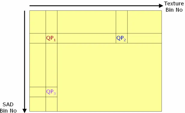
(36) record the accurate QP under the situation of current SAD and target number of bits for current frame or macroblock. With this method, there’s no need to worry about using a wrong R-D model. Therefore, the proposed method is more adaptive to variable video features. The method utilizes previous accurate data point to acquire one QP for encoding. When one frame or macroblock is to be encoded, the target number of bits and SAD value for current MB are utilized to index the table and acquire the QP. A large amount of interrupt service time for each MB executed in the system core is saved by implementing the h/w rate control with the lookup up table and other logic into the accelerator. Although the SAD and target number of bits are used in this approach, because the lookup table is also implemented in the accelerator core, the SAD could be pass directly from the motion estimator without interrupt to MCU.. 4.2.1. Process Flow of the H/W Rate Control Method There are three main processes for the table look-up method. The detail is described as follows. 4.2.1.1.. Modeling Table Initialization. What a rate control mechanism does is to select a quantization parameter according to the target bits of current frame or macroblock and complexity which shows how difficult to encode the residual and is measured as SAD or MSE. Quantization only affects the number of bits used to code quantized DCT coefficients. Therefore, the number of bits which codes texture and SAD are used to index the lookup table. Before indexing the lookup table to acquire a MB’s QP, one of the major issues is how to acquire the initial content of the modeling table. Here the initial modeling table is obtained from the result of encoding some sequence and this modeling table is saved into a storage device such as ROM. When encoding is started, the modeling table stored in the device is loaded into the memory for indexing. Experiments show that different contents of initial modeling table would not affect the coding result strictly.. 26.