電力系統中電壓崩潰偵測與電壓調節之研究

全文

(1)國立交通大學電機與控制工程學系碩士論文. 電力系統中電壓崩潰偵測與電壓調節之研究. STUDY OF VOLTAGE COLLAPSE DETECTION AND VOLTAGE REGULATION IN A POWER SYSTEM. 研究生：劉宏毅指導教授：梁耀文. 博士. 中華民國九十三年七月.

(2) 電力系統中電壓崩潰偵測與電壓調節之研究 STUDY OF VOLTAGE COLLAPSE DETECTION AND VOLTAGE REGULATION IN A POWER SYSTEM. 研究生：劉宏毅. Student：Hung-Yi Liu. 指導教授：梁耀文博士. Advisor：Yew-Wen Liang. 國立交通大學電機與控制工程學系碩士論文. A Thesis Submitted to Department of Electrical and Control Engineering College of Electrical Engineering and Computer Science National Chiao Tung University in Partial Fulfillment of the Requirements for the Degree of Master in Electrical and Control Engineering July 2004 Hsinchu, Taiwan, Republic of China. 中華民國九十三年七月.

(3) 電力系統中電壓崩潰偵測與電壓調節之研究. 研究生：劉宏毅. 指導教授：梁耀文博士. 國立交通大學電機與控制工程研究所. 摘. 要. 在本論文中，我們利用錯誤診斷濾波器設計一電壓崩潰的偵測方法。同時為了更進一步提升電力系統之電壓品質，我們利用可變結構控制法則設計一電壓調節器用以達到電壓調節的目的。此外，我們亦設計一負載估測器用以估測電力系統之負載變動，且在設計電壓調節器時，亦把負載的變動考慮進去，使我們所設計之電壓調節器有更好的調節能力。最後，我們把偵測電壓崩潰的機制引入我們所設計之電壓調節系統，提供電力系統一個安全、穩定且可靠的操作環境。. I.

(4) STUDY OF VOLTAGE COLLAPSE DETECTION AND VOLTAGE REGULATION IN A POWER SYSTEM. Student: Hung-Yi Liu. Advisor: Dr. Yew-Wen Liang. Department of Electrical and Control Engineering National Chiao Tung University. ABSTRACT In this thesis, we present a means of the detection of voltage collapse in a power system based on the linear-based fault identification filter (FIDF) design technique. Moreover, in order to promote the voltage quality of power supply for secure operation of a power system. We employ Variable Structure Control technique to design the voltage regulator of a power system. In addition, a load estimator is proposed to provide the accurate load variation to the VSC voltage regulator to have better regulating capacity. Finally, we combine the prior designs to maintain a secure and reliable operation of the power system.. II.

(5) 誌. 謝. 本篇論文的完成，實在要感謝太多人了，沒有你們的關心與協助，恐無法有所精進，希望日後能繼續給予指教與鼓勵，必銘記在心! 首先，特別要感謝我的指導教授梁耀文博士，感謝老師兩年多來細心與耐心的指導以及對我孜孜不倦的教誨，使我不僅在研究過程中受益良多，且在待人處世各方面均有許多的成長。也要感謝系上曾給予協助的老師，同時也要感謝口試委員廖德誠博士、鄭治中博士和宋朝宗博士給予指正與寶貴的建議，使得本論文不足之處得以補強。接下來，要感謝吳秉儒學長、朱自強學長及博士班徐聖棟學長在我遇到困難及心情低落時能給予適時的幫助與鼓勵，再來要感謝實驗室的同學煜寰，在學業及生活上給予支持與協助，而學弟信嘉對於我的論文研究幫助甚多、以及學弟嘉良，感謝你們對於我的幫助，使我能夠更專心於研究。感謝學長、學弟、同學以及所有我認識的朋友，有了你們的陪伴讓我的兩年研究生活顯得多采多姿且充滿回憶。最後要感謝我一生中最重要的家人，感謝我的父親、母親以及弟弟們，從小到大陪我一路走來，對我的包容，實在辛苦你們了!謹將此論文獻給你們，謝謝你們對於我的支持與鼓勵，讓我可以無後顧之憂的在學業上勇往直前，進而完成研究所的學業，謝謝你們!. 劉宏毅謹識民國九十三年七月. III.

(6) TABLE OF CONTENTS. CHINESE ABSTRACT ...............................................................................................................I ABSTRACT ...................................................................................................................................II ACKNOWLEDGEMENT .......................................................................................................III TABLE OF CONTENTS ..........................................................................................................IV LIST OF FIGURES ...................................................................................................................VI 1. INTRODUCTION ....................................................................................................................1 1.1. Motivation ..............................................................................................................................1 1.2. Outline .....................................................................................................................................4. 2. PRELIMINARIES ...................................................................................................................5 2.1. Fault Identification Filter(FIDF) ..........................................................................................5 2.2. Short-Time Fourier Transform ..............................................................................................8 2.2.1. Window function ..........................................................................................................8 2.2.2. Short-time Fourier transform .......................................................................................10 2.2.3. Time-Frequency Window ............................................................................................11 2.3. Variable Structure Control ..................................................................................................12 2.3.1. Sliding Surface ..............................................................................................................12 2.3.2. Variable Structure Control Design ..............................................................................17 2.4. Adaptive Control ..................................................................................................................20. 3. DETECTION OF VOLTAGE COLLAPSE FOR THE ELECTRIC POWER SYSTEMS .................................................................................................................................25 3.1. Dynamical Equations of Electric Power Systems .............................................................25 3.2. Voltage Collapse in the Electric Power Systems ...............................................................30 3.3. Results of FIDF Design .......................................................................................................31 IV.

(7) 3.4. Results of Signal Analysis ...................................................................................................37. 4. VOLTAGE REGULATION OF THE ELECTRIC POWER SYSTEMS ............41 4.1. Variable Structure Controller Design .................................................................................41 4.1.1. Controlled Power System Model ................................................................................41 4.1.2. Controller Design .........................................................................................................44 4.1.3. Simulation Results ........................................................................................................48 4.2. Parameter Estimator Design ...............................................................................................54 4.2.1. The Gradient Method ...................................................................................................54 4.2.1.1. Linear Parametrization Model ...........................................................................54 4.2.1.2. Predication-Error-Based Estimation Methods ..................................................55 4.2.1.3. The Gradient Estimator ......................................................................................56 4.2.1.4. Application To Power Systems ..........................................................................57 4.2.2. An Observer Approach .................................................................................................61 4.2.2.1. The Transformation of Decoupled Form ..........................................................61 4.2.2.2. Observer Design for Constant Parameters .......................................................62 4.2.2.3. Observer Design for Time-Varying Parameters ..............................................64 4.2.2.4. Application to Power Systems ..........................................................................66 4.3. Adaptive Control System Design .......................................................................................76 4.3.1. Control System Design ................................................................................................76 4.3.2. Application to Power Systems ....................................................................................77. 5. CONTROL OF VOLTAGE COLLAPSE .......................................................................82 5.1. Control of Voltage Collapse ................................................................................................83 5.2. Simulation Results ...............................................................................................................85. 6. CONCLUSIONS AND SUGGESTIONS FOR FURTHER RESEARCH ...........88 REFERENCES ............................................................................................................................90. V.

(8) LIST OF FIGURES. Figure 2.1. FIDF configuration ........................................................................................................7 Figure 2.2. Characteristic function....................................................................................................9 Figure 2.3. Time-frequency window for short-time Fourier transform( t * = ω * = 0 )................12. Figure 2.4. The sliding condition....................................................................................................14 Figure 2.5. Graphical interpretation of equations (2.23) and (2.24) ( n = 2 )..............................16 Figure 2.6. Chattering as result of imperfect control switching...................................................17 Figure 2.7. Filippov's construction of the equivalent dynamics in sliding mode.......................19 Figure 3.1. Power system model (a) original system (b) Th’evenin equivalent system ...........27 Figure 3.2. (a) load variation (Q 1). (b) load voltage (c) residual signal. (d) alarm by FIDF…………………………………………………….…………. 35 Figure 3.3. (a) load variation (Q 1). (b) load voltage (c) residual signal. (d) alarm by FIDF…………………………………………………….…………. 35 Figure 3.4. (a) load variation (Q 1). (b) load voltage (c) residual signal. (d) alarm by FIDF…………………………………………………….…………. 36 Figure 3.5. (a) load variation (Q 1). (b) load voltage (c) residual signal. (d) alarm by FIDF…………………………………………………….…………. 36 Figure 3.6. (a) Voltage response for Q 1 ñ 11.1 (b) residual signal (c) residual signal after averaging (d) spectrogram .........................................................................................38 Figure 3.7. Amplitude of the monitored frequency versus Q 1 ...................................................39 Figure 3.8. (a) residual signal for Q 1 ñ 11.1. (b) alarm by FIDF (c) amplitude of the. monitored frequency (d) alarm by monitored frequency......................................39 Figure 3.9. (a) load variation (b) residual signal (c) amplitude of the monitored frequency (d) alarm by monitored frequency...............................................................................40 VI.

(9) Figure 3.10. (a) load variation (b) residual signal (c) amplitude of the monitored frequency (d) alarm by monitored frequency.............................................................................40 Figure 4.1. The power system model with tap changer ...............................................................42 Figure 4.2. Q 1 = 11.2, x 0 = [0, 0, 0, 1.1] ...............................................................................51 Figure 4.3. Q 1 = 11.2, x 0 = [0.2, 0.2, 0.04, 0.98] ................................................................51 Figure 4.4. Q 1 = 11.2 + 0.1 sin(3t), x 0 = [0, 0, 0, 1.1] .....................................................52 Figure 4.5. Q 1 = 11.2 + 0.1 sin(3t), x 0 = [0.2, 0.2, 0.04, 0.98] ......................................52 Figure 4.6. Regulating Performance with Unknown Q 1 , x 0 = [0.2, 0.2, 0.04, 0.98] ........53 Figure 4.7. Regulating Performance with Unknown Q 1 , x 0 = [0.2, 0.2, 0.04, 0.98] ........53 Figure 4.8. Estimation for constant load Q 1 ñ 11 by Gradient method with. õ f = 10 and p o = 10 ..............................................................................................59 Figure 4.9. Estimation for constant load Q 1 ñ 11 by Gradient method with. õ f = 50 and p o = 10 ..............................................................................................59 Figure 4.10. Estimation for slow time-varying load Q 1 ñ 11 + 0.1 sin(0.5t) by Gradient method with õ f = 10 and p o = 10 ...............................................60 Figure 4.11. Estimation for fast time-varying load Q1 ñ 11 + 0.1 sin(5t) by Gradient method with õ f = 10 and p o = 10 ...............................................60 Figure 4.12. Estimation result by observer method for Q 1 = 11 and k1 = 10 , Q 1n = 11 ……………………………………………..…….71 Figure 4.13. Estimation result by observer method for Q 1 = 12 and k1 = 10 , Q 1n = 9 ……………………………………………….…….71 Figure 4.14. Estimation result by observer method for Q1 = 11 + 0.1 sin(t) and k 1 = 10 , Q 1n = 11 ......................................................................................72 Figure 4.15. Estimation result by observer method for Q 1 = 11 + 0.1 sin(10t) and k 1 = 10 , Q 1n = 11 ......................................................................................72. VII.

(10) Figure 4.16. Estimation result by observer method for Q 1 = 11 + 0.1 sin(10t) and k1 = 50 , Q 1n = 11 ......................................................................................73 Figure 4.17. Estimation result by observer method for Q1 = 11 + 0.1 sin(5t) and k 1 = 1 , Q 1n = 11 , ú = 0.2 , ñ = 0.01 , þ = 0.001 .........................73 Figure 4.18. Estimation result by observer method for Q1 = 11 + 0.1 sin(10t) and k 1 = 1 , Q 1n = 11 , ú = 0.2 , ñ = 0.01 , þ = 0.001 .........................74 Figure 4.19. Estimation result by observer method for 5% variation of Q 1 and k 1 = 10 , Q 1n = 10.8 ...................................................................................74 Figure 4.20. Comparisons of estimators with observer approach and gradient method............75 Figure 4.21. Estimation errors of observer approach and gradient method ...............................75 Figure 4.22. An adaptive control system........................................................................................76 Figure 4.23. Regulating performance and parameter estimation for Q1 = 11.2 ....................79 Figure 4.24. Regulating performance with Saturation control input...........................................79 Figure 4.25. System response..........................................................................................................80 Figure 4.26. Regulating performance and parameter estimation for. Q1 = 11 + 0.1 sin(5t) .........................................................................................81 Figure 5.1. A scheme of prevention of voltage collapse...............................................................84 Figure 5.2. (a) load variation (Q 1) (b) time response of load voltage without control (c) residual signal (d) alarm signal by FIDF (e) tap changer ratio n (f) time response of load voltage with control given by (e) .....................................86 Figure 5.3. (a) load variation (Q 1) (b) time response of load voltage without control (c) residual signal (d) alarm signal by FIDF (e) variation of tap changer ratio n (f) time response of load voltage with control given by (e) .....................................87. VIII.

(11) CHAPTER 1 Introduction. 1.1. Motivation. Recently, the study of power system stability has attracted lots of attention [6,28,34]. Among the possible instabilities, a serious type is the so-called “voltage collapse” [1,2,8,9,17,32]. This kind of instability in a power system is characterized by an initial slow progressive decline and then rapid decline in the voltage magnitude [17]. The voltage collapse behavior has been reported to be attributed to the increase of power demand that results in the operation of an electric power system near its stability limit [8,17]. In 1988, Dobson and Chiang [9] have presented a mechanism for voltage collapse and introduced a simple power system model containing a generator, an infinite bus and a nonlinear load. They claimed that the voltage collapse behavior might occur around a saddle node bifurcation point [8,9]. Abed et al. [1,2,32] have reported the oscillatory behavior of a power system using Hopf bifurcation theory. １.

(12) In addition to distinguishing the cause of voltage collapse, to detect such instability phenomena is also an important area of research. Traditional available methods have relied on utilizing system Jacobian matrix of power flow [4,16,21,37], by exploiting either its sensitivity by determining its vicinity to singularity or its eigenvalue behavior. These approaches have the drawback of time consuming computations. And with increased network size these Jacobian based methods will become very time consuming and therefore inappropriate for quick detection. Thus, the first goal in this thesis is to provide a means for quick detection of voltage collapse in the power system. Various techniques for fault detection of a control system have been developed (see e.g., [5,7]). Among these techniques, the so-called “fault identification filter’’ (FIDF) is one of the most effective [5,7]. The FIDF has been successfully applied to the detection of sensor fault [23], mobile robot [24] and compression systems [19]. In this thesis, we adopt the power system model proposed by Dobson and Chiang [9], and employ FIDF design technique to detect the voltage collapse. We will show how the FIDF may be used to detect the occurrence of voltage collapse in a power system without complex computations. In practical, an efficient and reliable operation of power systems should have the property that the voltage and frequency should remain nearly constant. As is well known, the frequency of a system is dependent on active power balance while the voltage magnitude is dependent on reactive power balance [16,27]. From voltage stability analysis, we know that the lack of the reactive power in the power system may cause the voltage decrease, which may in the worst case lead to the voltage collapse. So, an important issue for power system control is to maintain a steady acceptable voltage under normal operation and disturbed conditions, which is referred as the problem of voltage regulation. Thus, the second goal in this thesis is to provide a voltage controller which can achieve voltage regulation purpose. Tap changer is ２.

(13) known to be one of an effective device for voltage control. The effect of tap changer ratio in the power system has been studied in [20,22,39,16,27]. In this thesis, we will employ setting tap changer ratio to achieve voltage regulation. In practical, the power systems are large scale nonlinear systems. The simplest controller design for voltage regulation might be based on approximate linearization approach. However, this controller is usually effective around a neighborhood of operating point. In addition, the linearization approach might work well when a small disturbance occurs, but it usually cannot survive a large disturbance. Recently, nonlinear control theories have been employed to power systems voltage controller design. These designs are mainly based on the nonlinear feedback linearization technique [10,33,38], which transforms the power system into a linear and controllable one, and thus linear control theories can be applied to design an effective control law. Although the feedback linearization approach is a powerful tool for nonlinear controller design, it is only suitable for nonlinear affine systems (for definition, see e.g., [3]). Since in this thesis we take the tap changer as control input, the power system model is found to be a general nonlinear system form xç = f(x, u) in stead of being a nonlinear affine version. Thus feedback linearization approach can not be applied. It is known that variable structure control (VSC) has many advantages including fast response and small sensitivity to system uncertainties and disturbances [25,29]. It then has been widely applied to a variety of control problem, such as power system stability control [13,34,36], robotic control [15,26], and so on. In this thesis, we will adopt the VSC technique in the controller design issues. In many practical control problems, the controlled systems usually have parameter uncertainty. The uncertainty in power system may come from a large variation in loading condition during operation. It is known that the performance of a control system might not be acceptable or even result in unstable if it does not take the ３.

(14) parameter uncertainty into account for controller design. Thus, the third goal in this thesis is to provide a parameter estimation scheme to help voltage controller dealing with the power system in the presence of uncertainty or unknown variation in the load. Finally, we will develop a scheme of prevention of voltage collapse with the aid of prior analysis and design. It provides us a secure and reliable operation of the power system.. 1.2. Outline. The organization of this thesis is as follows. In Chapter 2, we recall some basic tool and theory. These include Fault Identification Filter, short-time Fourier transform, Variable Structure Control, Adaptive Control. In Chapter 3, we first introduce the model of power system proposed by Dobson and Chiang [9]. Then, we apply the FIDF to the detection of voltage collapse in a power system. In Chapter 4, we establish the model of power system with tap changer. Then, the Variable Structure Control scheme is applied to adjust the tap changer ratio for the purpose of voltage regulation. In Chapter 5, a scheme of prevention of voltage collapse is proposed, and Simulation results demonstrate the effectiveness of this scheme. Finally, conclusions and suggestions for further research are given in Chapter 6.. ４.

(15) CHAPTER 2 Preliminaries. In this chapter we review some basic tool and theory. These include Fault Identification Filter [5,18], short-time Fourier transform [11], Variable Structure Control [25,29], adaptive control [25]. These results will be employed in the next two chapters to develop the detection of voltage collapse and voltage regulation for the electric power system.. 2.1. Fault Identification Filter (FIDF). Fault Identification Filter is a tool that can provide an efficient approach to detect the appearance of faults in a control system. In this section we recall the FIDF design results presented in [5].. ５.

(16) Consider a linear system is given by x& (t ) = Ax(t ) + Bu (t ) + E1 f (t ). (2.1). y (t ) = Cx (t ) + Du (t ) + E 2 f (t ). (2.2). where x(t ) ∈ ℜ n , u (t ) ∈ ℜ m , f (t ) ∈ ℜ q , and y (t ) ∈ ℜ p denote the state vector, the input vector, the fault vector, and the output vector, respectively. From (2.1) and (2.2), by taking Laplace transform, we have y ( s ) = Gu ( s )u ( s ) + G f ( s ) f ( s ). (2.3). where. and. Gu ( s ) = C ( sI − A) −1 B + D. (2.4). G f ( s) = C ( sI − A) −1 E1 + E 2. (2.5). The object of FIDF design is to obtain two proper and stable filters H 1 ( s ) and H 2 ( s) such that the residual vector. r ( s) = H 1 ( s )u ( s ) + H 2 ( s) y ( s). (2.6). r ( s ) → 0 if and only if f ( s ) → 0. (2.7). has the following property :. From Eqs. (2.3)-(2.6), we have. r ( s ) = [ H 1 ( s ) + H 2 ( s )Gu ( s )]u ( s ) + H 2 ( s )G f ( s ) f ( s ). ６. (2.8).

(17) The configuration of a FIDF is shown in Figure 2.1.. u. y. PLANT. H1(s). +. H2(s). r (s ). Figure 2.1: FIDF configuration. To fulfill the requirement of (2.7), we first assume that G f (s ) as given by (2.5) is invertible. The FIDF design procedure is given in [5] then can be summarized as the following algorithm. Algorithm 1 (FIDF design procedure). Step 1 : Construct H 2 ( s) so that the transfer matrix H 2 ( s )G f ( s ) is a diagonal proper. and stable one.. Step 2 : Determine H 1 (s) such that H 1 ( s) + H 2 ( s)Gu ( s ) = 0. Step 3 : Establish and check r (s) according to Eq. (2.6). ７.

(18) Under the procedure of Algorithm 1, it is noted from Eq. (2.8) that the residual vector is influenced only by the fault vector. Thus, by properly checking the value of residual vector as listed in Step 3 of Algorithm 1 above, one can detect the system fault accurately. In addition to the effect of fault vector, the system output is also affected by nonzero initial state. Since the objective is that the residual be affected only by the fault vector, The response to a nonzero initial state should decay to zero. This implies that the matrix A in Eq. (2.1) should also be required to be stable.. 2.2 Short-Time Fourier Transform. The short-time Fourier transform is the most widely used method for studying nonstationary signals. The concept behind it is simple and powerful. Break up the signal into small time segments and Fourier analyze each time segment to ascertain the frequencies that existed in that segment. That is the basic idea of the Short-time Fourier Transform. The totality of such spectra indicates how the spectrum is varying in time.. 2.2.1. Window function. If we are interesting in a desired portion of a signal at time t , it can be obtained by multiplying the original signal by a window function, which emphasizes the signal at that time interval, centered at t , and suppresses the signal at other times. Let φ (t ) be a real-valued window function. Then we apply the window function to the original signal and obtain the information of f (t ) near t = b , and express this as f (t )φ (t − b) =: f b (t ) . In particular, if φ (t ) =: χ [ −τ ,τ ) (t ) , as shown in figure2.2, then ⎧ f (t ), t ∈ [b − τ , b + τ ) f b (t ) = ⎨ otherwise. ⎩ 0, ８. (2.9).

(19) where b is a sliding factor and we can slide the window function along the time axis to analyze the local behavior of the function f (t ) in different intervals.. χ [ −τ ,τ ) (t ). −τ. τ. 0. Figure2.2: Characteristic function. In the window function, We have the two most important parameters, its center and width. It is clear that the center and the standard width of the window function in Figure2.2 are 0 and 2τ , respectively. For a general window function φ (t ) , we define its center t * as t * :=. 1. φ. 2. ∫. ∞. −∞. 2. t φ (t ) dt. (2.10). and the root-mean-square (RMS) radius ∆ φ as 1 ⎡ ∞ 2 ∆ φ := (t − t * ) 2 φ (t ) dt ⎤ ∫ ⎢ ⎥⎦ − ∞ φ ⎣. 1. 2. (2.11). The function is called a time window. For the window of Figure2.2, use (2.10) and (2.11) to verify that t * = 0 and ∆ φ = τ / 3 . Therefore, the RMS width is smaller than the standard width by a factor of 1 / 3 .. ９.

(20) From the function φ (t ) described above, similarly, we can have a frequency window φˆ(ω ) with center ω * and the RMS radius ∆ φˆ defined analogous to (2.10) and (2.11) as. ω * :=. 1. φˆ. 2. ∫. ∞. −∞. 2. ω φˆ(ω ) dω. 2 1 ⎡ ∞ * 2 ˆ ( ω ω ) φ ( ω ) dω ⎤ ∆ φˆ := − ∫ ⎥⎦ ⎢ − ∞ φˆ ⎣. (2.12). 1. 2. (2.13). Theoretically, A function cannot be limited in time and frequency simultaneously. Verifying φ (t ) for the window of Figure2.2, ω * = 0 and ∆ φ = ∞ , this window is the best time window but the worst frequency window.. 2.2.2. Short-time Fourier transform. We want to obtain the properties of a signal f (t ) in the neighborhood of some desired location in time t = b , by multiplying an appropriated window function φ (t ) to produce the windowed function f b (t ) = f (t )φ (t − b) and then taking the Fourier transform of f b (t ) . This is the short-time Fourier transform (STFT). Formally, we can define the STFT of a function f (t ) with the window function φ (t ) discussed in Section 2.2.1 in the time-frequency plane as Gφ f (b,ξ ) := ∫. ∞. −∞. f (t )φ b,ξ (t )dt. (2.14). where. φ b ,ξ ( t ) := φ ( t − b ) e jξ t. (2.15). Because of the windowing nature of the STFT, this transform is referred to as the windowed Fourier transform.. １０.

(21) 2.2.3. Time-Frequency Window. Let us consider the window function φ (t ) in (2.15). If t * is the center and ∆ φ the radius of the window function, then (2.14) gives the information of the function f (t ) in the time window: [t * + b − ∆ φ , t * + b + ∆ φ ]. (2.16). To derive the corresponding window in frequency domain, apply Parseval’s identity to (2.14). We have Gφ f (b, ξ ) := ∫. ∞. −∞. =. f (t )φ (t − b)e − jξ t dt. (2.17). 1 − jξ b ∞ ˆ e ∫ f (ω )φˆ(ω − ξ )e − jbω dω −∞ 2π. [. ]. ∨ = e − jξ b fˆ (ω )φˆ(ω − ξ ) (b). (2.18). where the symbol “ ∨ ” represents the inverse Fourier transform. Observe that (2.17) has a form similar to (2.14). If ω * is the center and ∆φˆ is the radius of the window function φˆ(ω ) , then (2.17) gives us information about the function fˆ (ω ) in the interval [ω * + ξ − ∆φˆ, ω * + ξ + ∆φˆ]. (2.19). Because of the similarity of representation in (2.14) and (2.17), the STFT give information about the function f (t ) in the time-frequency widow: [t * + b − ∆ φ , t * + b + ∆ φ ] × [ω * + ξ − ∆φˆ, ω * + ξ + ∆φˆ]. (2.20). Figure 2.3 represents graphically the notion of the time-frequency windowgiven by (2.19). Here we have assumed that t * = ω * = 0 .. １１.

(22) ω. 2∆ φ. ξ2. 2 ∆ φˆ. 2∆ φ. ξ1. 2 ∆ φˆ. 2∆ φ. ξ0. 2 ∆ φˆ. b0. b1. b2. t. Figure 2.3: Time-frequency window for short-time Fourier transform( t * = ω * = 0 ). 2.3 Variable Structure Control The Variable Structure Control(VSC) have the advantages of faster response and smaller sensitivity to system uncertainties and disturbances. In this thesis, we will adopt VSC schemes to design our controller. In this section we review some basic concept of VSC theory first. 2.3.1. Sliding Surface. Consider a single-input dynamic system. x ( n ) = f ( x) + b( x)u. (2.21). where the scalar x is the output of interest, the scalar u is the control input, and X = [x. x& K x ( n−1) ]T is the state vector. In system (2.21), the functions f (x). and b(x) (in general, nonlinear) are not exactly known, but the extent of the imprecision on f (x) is upper bounded by a known continuous function of x , and control gain b(x) is of known sign and bounded by a known continuous function of x , respectively. For example, the inertia of a mechanical system is only known to a. certain accuracy, and friction models only describe part of the actual friction forces. １２.

(23) The control problem is to get the state x to track a specific time-varying state X d = [ xd. x& d. K xd. ( n −1) T. ]. in the presence of model uncertainty on f (x) and. b(x) . For the tracking task by using a finite control u , the initial desired state xd (0) must be such that : xd (0) = x(0). (2.22). In a second-order system, for example, position or velocity can not "jump", so that any desire trajectory feasible from t = 0 necessarily starts with the same position and velocity as those of the plant. Otherwise, tracking can only be achieved after a transient. x = x − xd is the tracking error in the variable x , and let Define ~ ~ x = x − xd = [ ~ x. ~ x& K ~ x ( n−1) ]T. to be the tracking error vector. Furthermore, let us define a time-varying surface S (t ) in the state-space R (n ) by the scalar equation s ( X ; t ) = 0 , where s( X ; t ) = (. d + λ ) n−1 ~ x dt. (2.23). Given initial condition (2.22), the tracking problem X ≡ X d is equivalent to that of remaining on the surface S (t ) for all t > 0 ; indeed s ≡ 0 represents a linear x ≡ 0 , given initial conditions (2.22). differential equation whose unique solution is ~. Thus, the problem of tracking the n-dimensional vector xd can be reduced to that keeping the scalar portion s at zero. More precisely, the problem of tracking the n-dimensional vector xd can in effect be replaced by a 1st − order stabilization problem in s . Indeed, since from (2.23) the expression of s contains ~ x ( n−1) , we only need to differentiate s once for the input u to appear. Furthermore, bounds on s can be directly translated into bounds on the tracking error vector ~ x , and. １３.

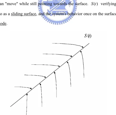
(24) therefore the scalar s represents a true measure of tracking performance. Then,. 1st − order problem of keeping the scalar s at zero can be achieved by choosing the control law u of the system (2.21) such that outside of S (t ) 1d 2 s ≤ −η s 2 dt. (2.24). where η is a strictly positive constant. Practically, (2.24) states that the squared "distance" to the surface, as measured by s 2 , decrease along system trajectory. Thus, it constrains trajectories to points towards the surface S (t ) , as illustrated in Figure 2.4. In particular, once on the surface, the system trajectories remain on the the surface. In other words, satisfying sliding condition (2.24), makes the surface an invariant set. Furthermore, as we shall see, (2.24) also implies that some disturbances or dynamics uncertainties can be tolerated while still keeping the surface an invariant set. Graphically, this corresponds to the fact that in Figure 2.4 the trajectories off the surface can "move" while still pointing towards the surface. S (t ) verifying (2.24) is referred to as a sliding surface, and the system's behavior once on the surface is called sliding mode.. Figure 2.4: The sliding condition １４.

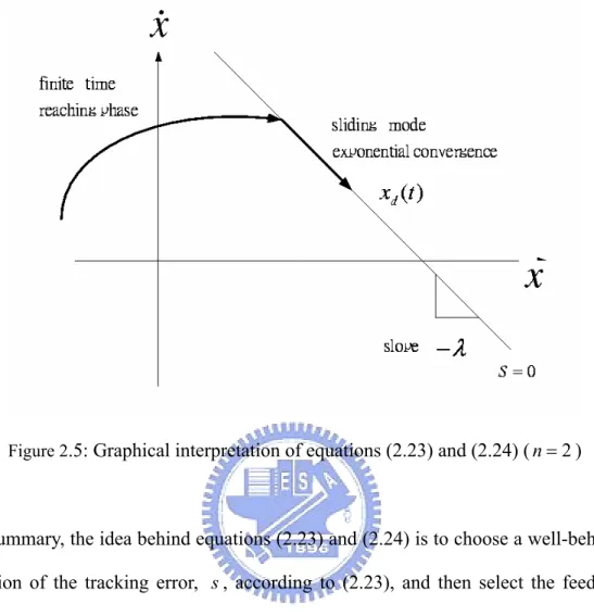
(25) The other interesting appearance of the invariant set S (t ) is that once on it, the system trajectories are defined by the equation of the set itself, namely (. d + λ ) n−1 ~ x =0 dt. In other words, the surface S (t ) is both a place and a dynamics. This fact is simply the geometric interpretation of the definition (2.23) allow us, in effect, to replace an. n th − order problem by a 1st − order one. Finally, satisfying (2.24) guarantees that if condition (2.22) is not exactly verified, ie., if X (t = 0) is actually off X d (t = 0) , the surface S (t ) will yet be reached in a finite time smaller than s (t = 0) /η . Indeed, assume for instance that s (t = 0) > 0 , and let t reach be the time required to hit the surface s = 0 . Integrating (2.24) between t = 0 and t = t reach leads to 0 − s (t = 0) = s (t = t reach ) − s(t = 0) ≤ −η (t reach − 0) while implies that t reach ≤ s (t = 0) /η Furthermore, definition (2.23) implies that once on the surface, the tracking error tends exponentially to zero, with a time constant (n − 1) / λ (form the sequence of (n − 1) filters of time constants equal to 1 / λ . The typical system behavior implied by satisfying sliding condition (2.24) is illustrated in Figure 2.5 for n = 2 . The sliding surface is a line in the phase plane, of slope − λ and containing the (time-varying) point X d = [ X d. X& d ]T . Starting from. any initial condition, the state trajectory reaches the time-varying surface in a finite time smaller than s (t = 0) /η , and then slide along the surface towards X d exponentially, with a time-constant equal to 1 / λ .. １５.

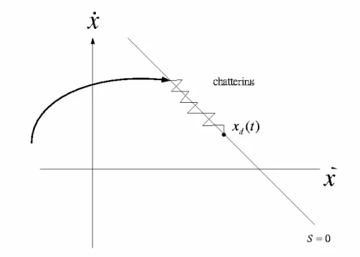
(26) Figure 2.5: Graphical interpretation of equations (2.23) and (2.24) ( n = 2 ). In summary, the idea behind equations (2.23) and (2.24) is to choose a well-behaved function of the tracking error, s , according to (2.23), and then select the feedback control law u in system (2.21) such that s 2 remains a Lyapunov-like function of the closed-loop system, despite the presence of model uncertainties and disturbances. The controller design procedure then consists of two steps. First, a feedback control law u is selected so as to verifying sliding condition. However, in order to account for the presence of modeling uncertainties and disturbances, the control law has to be discontinuous across S (t ) . Since the implementation of the associate control switchings is necessarily imperfect (for example, in practice switching is not instantaneous, and the value s is not known with infinite precision), this leads to chattering as showing in Figure 2.6.. １６.

(27) Figure 2.6 Chattering as result of imperfect control switching. The chattering is undesirable in practice, since it involves high control activity and further may excite high-frequency dynamics neglected in the course of modeling (such as unmodeled structure modes, neglected time-delays, and so on). Thus, in a second step, the discontinuous control law u is suitably smoothed to achieve an optimal trade-off between control bandwidth and tracking precision: while the first step accounts for parametric uncertainty, the second step achieves robustness to high-frequency unmodeled dynamics.. 2.3.2. Variable Structure Control Design. The implementation of the Variable Structure Control (VSC) consists of two main phases. First, we should construct the sliding surface such that the system states restricted to the sliding surface will produce the desired behavior. Second, we construct switched feedback gain which derive the plant state trajectory to the sliding surface in finite time and restrict the state to sliding surface. The method of equivalent control is means of determining the system motion restricted to the sliding surface. １７.

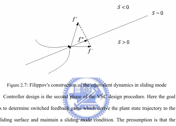
(28) Suppose at t 0 , the state trajectory of the plant intercepts the sliding surface and a sliding mode exists for all t > t 0 . The existence of a sliding mode implies (1) s& = 0 , and (2) s = 0 for all t > t 0 . The system's motions on the sliding surface can be given an interesting geometric interpretation, as an "average" of the systems' dynamics on both sides of the surface. The system while in sliding mode can be written as s& = 0. (2.25). By solving the above equation formally for the control input, we obtain an expression for u called the equivalent control, u eq which can be interpreted as the continuous control law that would maintain s& = 0 if the dynamics were exactly known. For example, for a second-order system &x& = f + u. (2.26). In order to have the system track x(t ) = xd (t ) , we define a sliding surface s = 0 according to (2.23), namely: s=(. d + λ )~ x =~ x& + λ~ x dt. (2.27). We then have: s& = &x& − &x&d + λ~ x& = f + u − &x&d + λ~ x&. (2.28). the equivalent control u eq of a continuous control law that would achieve s& = 0 is u eq = − f + &x&d − λ~ x&. (2.29). and the system dynamics while in sliding mode is &x& = f + u eq = &x&d − λ~ x&. (2.30). Geometrically, the equivalent control can be constructed as u eq = αu + + (1 − α )u −. (2.31). i.e., as a convex combination of the value of u on both sides of the surface S (t ) . The value of α can again be obtained formally from (2.25), which corresponds to. １８.

(29) requiring the system trajectories be tangent to the surface. This intuitive construction i s s u mma ri ze d i n F i g u r e 2 .7, where f − = [ x&. f + u − ]T and f eq = [ x&. f + = [ x&. f + u + ]T , and similarly. f + u eq ]T . Its formal justification was derived in. the early 1960's by the Russian mathematician A.F.Filippov.. Figure 2.7: Filippov's construction of the equivalent dynamics in sliding mode. Controller design is the second phase of the VSC design procedure. Here the goal is to determine switched feedback gains which derive the plant state trajectory to the sliding surface and maintain a sliding mode condition. The presumption is that the sliding surface has been designed. Among several approach (e.g. the diagonalization method and hierarchical control method), augmenting the equivalent control is one popular approach. This structure of control of system (2.26) is. u = u eq + u re. (2.32). where u re is the discontinuous or the switched part of (2.32). Consider the system x& . In order to satisfy sliding condition (2.24), we (2.26), we have u eq = − f + &x&d − λ~. add to u re a term discontinuous across the surface s = 0 , and let u = u eq = u eq. + u re. (2.33). − k sgn(s ). １９.

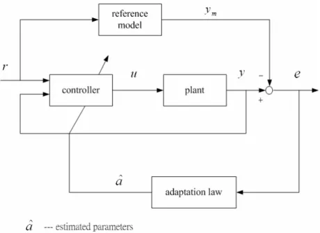
(30) where sgn is the sign function ⎧ 1 if ⎪ sgn( s ) = ⎨ 0 if ⎪− 1 if ⎩. s>0 s=0. (2.34). s<0. By selecting k to be a positive scalar, then 1d 2 s = s& ⋅ s = − k sgn( s) ⋅ s = − k s ≤ −η s 2 dt For k is large enough, we can guarantee that (2.24) is verified.. 2.4 Adaptive Control. Many dynamic systems to be controlled have constant or slowly-varying uncertain parameters. For instance, Power systems may be subjected to large variations in loading conditions. Adaptive control is an approach to the control of such system. The basic idea in adaptive control is to estimate the uncertain plant parameters (or, equivalently, the corresponding controller parameters) on-line based on the measured system signal, and use the estimated parameters in the control input computation. An adaptive control system can thus be regarded as a control system with on-line parameter estimation. An adaptive controller differs from an ordinary controller in that the controller parameters are variable, and there is a mechanism for adjusting these parameters on-line based on signals in the system. There are two main approaches for constructing adaptive controllers. One is the so-called model-reference adaptive control method, and the other is the so-called self-tuning method.. ２０.

(31) Model-reference adaptive control (MRAC). Generally, a model-reference adaptive control system can be schematically represented by Figure 2.8. It is composed of four parts: a plant containing unknown parameters, a reference model for compactly specifying the desired output of the control system, a feedback control law containing adjustable parameters, and an adaptation mechanism for updating the adjustable parameters.. Figure 2.8 A model-reference adaptive control system. The plant is assumed to have a known structure, although the parameters are unknown, for linear plants, this means that the number of poles and the number of zeros are assumed to be known, but that the locations of these poles and zeros are not. For nonlinear plants, this implies that the structure of the dynamic equations is known, but that some parameters are not. A reference model is used to specify the ideal response of the adaptive control system to the external command. Intuitively, it provides the ideal plant response which the adaptation mechanism should seek in adjusting the parameters. The choice ２１.

(32) of the reference model is part of the adaptive control system design. This choice has to satisfy two requirements. On the one hand, it should reflect the performance specification in the control tasks, such as rise time, settling time, overshoot or frequency domain characteristics. On the other hand, this ideal behavior should be achievable for the adaptive control system, i.e., there are some inherent constraints on the structure of the reference model (e.g., its order and relative degree) given the assumed structure of the plant model. The controller is usually parameterized by a number of adjustable parameters (implying that one may obtain a family of controllers by assigning various values to the adjustable parameters). The controller should have perfect tracking capacity in order to allow the possibility of tracking convergence. That is, when the plant parameters are exactly known, the corresponding controller parameters should make the plant output identical to that of the reference model. When the plant parameters are not known, the adaptation mechanism will adjust the controller parameters so that perfect tracking is asymptotically achieved. If the control law is linear in terms of the adjustable parameters, it is said to be linearly parameterized. Existing adaptive control designs normally require linear parametrization of the controller in order to obtain adaptation mechanisms with guaranteed stability and tracking convergence. The adaptation mechanism is used to adjust the parameters in the control law. In MRAC systems, the adaptation law searches for parameters such that the response of the plant under adaptive control becomes the same as that of the reference model, i.e., the objective of the adaptation is to make the tracking error converge to zero. Clearly, the main difference from conventional control lies in the existence of this mechanism. The main issue in adaptation design is to synthesize an adaptation mechanism which will guarantee that the control system remains stable and the tracking error converges to zero as the parameters are varied. Many formalisms in nonlinear control can be ２２.

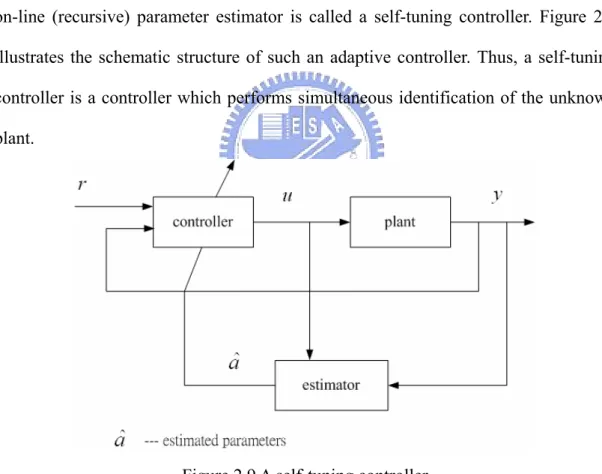
(33) used to this end, such as Lyapunov theory, hyperstability theory, and passivity theory. Although the application of one formalism may be more convenient than that of another, the results are often equivalent.. Self-tuning controllers (STC). In non-adaptive control design (e.g., pole placement), one computes the parameters of the controllers from those of the plant. If the plant parameters are not known, it is intuitively reasonable to replace them by their estimated values, as provided by a parameter estimator. A controller thus obtained by coupling a controller with an on-line (recursive) parameter estimator is called a self-tuning controller. Figure 2.9 illustrates the schematic structure of such an adaptive controller. Thus, a self-tuning controller is a controller which performs simultaneous identification of the unknown plant.. Figure 2.9 A self-tuning controller The operation of a self-tuning controller is as follows: at each time instant, the estimator sends to the controller a set of estimated plant parameters, which is computed based on the past plant input u and output y ; the computer finds the corresponding controller parameters, and then computes a control input u based on. ２３.

(34) the controller parameters and measured signals; this control input u causes a new plant output to be generated, and the whole cycle of parameter and input updates is repeated. Note that the controller parameters are computed from the estimates of the plant parameters as if they were the true plant parameters. This idea is often called the certainty equivalence principle. Parameter estimation can be understood simply as the process of finding a set of parameters that fits the available input-output data from a plant. This is different from parameter adaptation in MRAC systems, where the parameters are adjusted so that the tracking errors converge to zero. For linear plants, many techniques are available to estimate the unknown parameters of the plant. The most popular one is the least-squares method and its extensions. There are also many control techniques for linear plants, such as pole-placement, PID, LQR (linear quadratic control), minimum variance control, or H ∞ designs. By coupling different control and estimation schemes, one can obtain a variety of self-tuning regulators. The self-tuning method can also be applied to some nonlinear systems without any conceptual difference. In the basic approach to self-tuning control, one estimates the plant parameters and then computes the controller parameters. Such a scheme is often called indirect adaptive control, because of the need to translate the estimated parameters into controller parameters. It is possible to eliminate this part of the computation. to do this, one notes that the control law parameters and plant parameters are related to each other for a specific control method. This implies that we may reparameterize the plant model using controller parameters (which are also unknown, of course), and then use standard estimation techniques on such a model. Since no translation is needed in this scheme, it is called a direct adaptive control scheme. In MARC systems, one can similarly consider direct and indirect ways of updating the controller parameters. ２４.

(35) CHAPTER 3 Detection of Voltage Collapse for the Electric Power Systems. In this chapter, we first introduce the dynamical equations of electric power systems that proposed by Dobson and Chiang [9]. Then, we apply the FIDF and signal analysis tool to the detection of voltage collapse in a power system.. 3.1. Dynamical Equations of Electric Power Systems. It is known that load characteristic has a significant effect on a power system dynamics [6,35]. Therefore the voltage collapse cannot be studied using classical models, such as constant PQ, constant impedance, and constant current models, which ２５.

(36) assume the magnitude of the load voltage to be constant. In this thesis, we adopt the power system model from Dobson and Chiang [9] as below:. The Load Model: The nonlinear load model (3.1)-(3.2) below is originally. introduced by Walve [31] and then modified by [9]. It includes a dynamic induction motor model with a constant PQ load. The combined model for the motor and the PQ load has the following form:. à á P = P0 + P1 + Kpwîç + Kpv + V + TVç. Q = Q0 + Q1 + K qw îç + K qvV + K qv2V2. (3.1) (3.2). where P0 and Q0 are the constant real and reactive powers of the motor, P 1 and. Q1 represent the PQ load, and the remaining parameters are same as those given in [9].. The Power System Model: The power system model in this thesis is adopted from. Dobson and Chiang [9] as shown in Figure 3.1.(a). In this model, one generator is a slack bus while the other has constant voltage magnitude Em and angle îm satisfies the following swing equation:. Mî¨m = à dmω + P m + EmVY m sin (î à î m à ò m) + E2mY m sin ò m. where M ,. dm. (3.3). and P m denote the generator inertia, damping and mechanical. power, respectively. In the model, Q1 is chosen as the system parameter so that increasing Q1 corresponds to increasing the load reactive power demand. In addition, the load also includes a fixed capacitor C to raise the voltage up to near 1.0 per unit. ２６.

(37) To facilitate the analysis, it is convenient to account for the capacitor by adjusting E0 and Y 0 to give the Th’evenin equivalent of the circuit with the capacitor. The adjusted values are. à á 1/2 à1 E 00 = E 0/ 1 + C 2Y à2 0 à 2CY 0 cos ò 0. ð ñ1/2 à1 cos 2 à Y00 = Y0 1 + C2Yà2 ò CY 0 0 0. ò00. = ò0 + tan. à1. ú. CYà1 sin ò0 0 1àCYà1 cos ò0 0. û. (3.4). (3.5). (3.6). Obviously, the product E00Y00 and E0Y0 are being the same constant. Then we have the equivalent circuit as shown in Figure 3.1.(b).. Figure 3.1: Power system model (a) original system (b) Th’evenin equivalent system ２７.

(38) By calculating VIã of the network, the real and reactive powers supplied by the network are P = à E 00Y 00V sin (î + ò0) à E mY mV sin (î à îm + òm) à á + Y 00 sin ò 00 + Y m sin ò m V 2. (3.7). Q = E 00Y 00V cos (î + ò 0) + E mY mV cos (î à î m + ò m) à á à Y 00 cos ò00 + Y m cos òm V 2. (3.8). From Eqs. (3.3) and equating (3.1)-(3.2) with (3.7)-(3.8), we have the overall dynamical equations for the electric power system as below:. îçm = ω. (3.9). Mωç = à d mω + P m + E mY mV sin (î à î m à ò m). + E 2mY m sin ò m. (3.10). K qwîç = à K qv2V 2 à K qvV + Q (î m, î, V) à Q 0 à Q 1. (3.11). TK qwK pvVç = K pwK qv2V 2 + (K pwK qv à K qwK pv) V + K qw (P(î m, î, V) à P 0 à P 1) à K pw (Q(î m, î, V) à Q 0 à Q 1). (3.12). where. Q(î m, î, V) = E 00 Y 00 V cos (î + ò 0 ) + E mYmV cos (î à î m + ò m) à á à Y 00 cos ò 00 + Y m cos ò m V 2. (3.13). P(î m, î, V) = à E 00 Y 00 V sin (î + ò 0 ) à E mY mV sin (î à î m + ò m) à á à Y 00 sin ò 00 + Y m sin ò m V 2. ２８. (3.14).

(39) In this thesis, the system parameters are adopted from [9] as follows: The load parameters are. K pw = 0.4, K pv = 0.3, K qw = à 0.03, K qv = à 2.8,. K qv2 = 2.1, T = 8.5, P 0 = 0.6, Q 0 = 1.3, P 1 = 0 The network and generator parameters are. Y 0 = 20.0, ò 0 = à 5.0, E 0 = 1.0, C = 12.0, Y00 = 8.0, ò00 = à 12.0, E00 = 2.5, Ym = 5.0,. ò m = à 5.0, E m = 1.0, P m = 1.0, d m = 0.05, M = 0.3 All parameters are in per unit expect for angles, which are in degrees. Let x 1 = î m, x 2 = ω, x 3 = î, x 4 = V . Then Eqs. (3.9)-(3.12) can be written in the form of xç = f ( x, u ) , u = Q 1 as below: (3.13). xç1 = x 2. à áá xç2 = 3.33333 (0.56422 à 0.05x 2 + 5x 4 sin (0.08727 à x 1 + x 3) (3.14). xç3 = à 33.33333 (à 1.3 à Q1 + 2.8x4 à 15.00486x24. + 20x 4 cos (0.08727 à x 3) + (5x 4 cos (0.08727 + x 1 à x 3))). (3.15). à à xç4 = à 13.0719 à 1.111x4 + 0.84x24 à 0.4 à 1.3 à Q1 à 12.90486x24. + 20x4 cos (0.08727 à x3) + 5x4 cos (0.08727 + x1 à x3)). à à 0.03 à 0.6 à 2.17889x24 + 20x4 sin (0.08727 à x3). + 5x 4 sin (0.08727 + x 1 à x 3). áá. (3.16). The system equilibrium points can then be obtain by solving f ( x, Q 1) = 0 , which depends on the load reactive power parameter Q 1 .. ２９.

(40) 3.2. Voltage Collapse in the Electric Power Systems. The study of power system stability has attracted lots of attention (see e.g., [6,28,34] and the references therein). Among the possible instabilities, a serious type is the so-called “voltage collapse.’’ This kind of instability in a power system is characterized by an initial slow progressive decline and then rapid decline in the voltage magnitude [17]. Two typical examples are shown in Figures 3.5(a) and 3.2(b). The voltage collapse behavior has been reported to be attributed to the increase of power demand that results in the operation of an electric power system near its stability limit [9,16,17]. As is well known, the qualitative change in the behavior of a nonlinear system with the change of one or more parameters is due to bifurcations. The variations of any parameter might result in complicated behavior and even give rise to system instabilities. Among the researches, for instance, Thomas and Tiranuchit [28] have pointed out that the induction motor dynamics could affect the voltage stability. Dobson and Chiang [8,9] have presented a mechanism for voltage collapse and introduced a simple power system model containing a generator, an infinite bus and a nonlinear load. They claimed that the voltage collapse behavior might occur around a saddle node bifurcation point. Abed et al. [1,2,32] have reported the oscillatory behavior of a power system using Hopf bifurcation theory.. ３０.

(41) 3.3. Results of FIDF Design. In this section, the FIDF technique will be employed to detect the occurrence of voltage collapse in a power system described in Section 3.2. It is observed that, when system experiences a heavy load, the voltage might exhibit a growing oscillation and then sudden breakdown if the load exceeds a critical value, however, the scenario do not happen for it's linearized model. With this observation, a linear-based fault identification filter (FIDF) design technique is proposed to detect the voltage collapse. This is achieved by treating the difference between the output of the power system and that of its linearized model at a stable operating point as a fault vector and then investigating the effect of the fault on the designed FIDF. In order to apply the FIDF results [5], we should construct the linearized model of the system (3.13)-(3.16) about an asymptotically stable operating point. x T0 (Q 10) = (x 10, x 20, x 30, x 40) T for some given Q 1 = Q 10 as follows:. x êç = Ax ê + BQê1. (3.17). ê = x à x 0 and Qê1 = Q1 à Q10 . Moreover, we assume that the available where x output of the power system has the form. y = Cx ê + DQê1 ,. (3.18). where C ∈ R pân and D ∈ R pâm are two constant matrices. It is known that a linear model derived from a nonlinear one is a close approximation only near the operating point. To reduce the influence of the difference between the two models, it is suggested that the stable operating point for the power system be chosen to be close to the instability inception point. In this section the operating point is chosen to be close to the first Hopf bifurcation point.. ３１.

(42) Denote y non(t) and y lin(t) the output for nonlinear and linear model, respectively. It is noted that the two outputs y non(t) and y lin(t) are not equal in general. It is shown in [18] that the steady state output of the linearized model is linearly dependent on the input. We describe briefly as follow: For the linearized model (3.17), (3.18), it is known that. ⎧t y lin(t) = Ce Atx ê(0) + ⎭ Ce A(tàü)BQê1(ü)dü + DQê1(t) 0. (3.19). The first term on the right hand side of (3.19) depends only on the initial state while the second and third terms depend only on the input. Since the matrix A given in. ê(0) → 0 as t → ∞ . The input and (3.17) is a Hurwitz matrix. It follows, Ce Atx output of the linearized model has the following relationship.. Y(s) = [C(sI à A) à1B + D]Q(s). (3.20). ê1(t) a n d w h e r e Q(s) a n d Y(s) a r e t h e L a p l a c e t r a n s f o r m s o f Q. y lin(t) à Ce Atx ê(0) , respectively. If the reactive power demand maintains a constant Qê 1 = Q 11 . By Final Value Theorem and A is stable, we have. lim y lin(t) à Ce Atx ê(0). t→∞. = lim sY(s) s→0. = Q 11(à CAà1B + D). (3.21). This means that the steady state output of the linearized model is linearly dependent on the input. However, when voltage collapse happens, the load voltage of the nonlinear model will exhibits a growing oscillatory voltage transient prior to voltage collapse. With these observations, the idea is to treat the difference. y non à y lin as a fault vector and then apply the FIDF technique to inspect the effect on this fault vector before voltage collapse occurs. In these simulations, we choose the load voltage V as the output which is easily measured. The output is then in the form ３２.

(43) of (3.18) with C = (0 0 0 1) and D = 0. (3.22). for both the linear and nonlinear models.. It was shown from bifurcation analysis that the voltage collapse might occur when. Q 1 is near the Hopf bifurcation point 10.89 [1,2,39]. This motivates us to choose the T operating point at Q 1 = 10.8 , which gives x0 = (0.1829, 0, à 0.0068, 1.1031) as. an equilibrium point. The matrix A given in (3.17) is found to be Hurwitz with eigenvalues {à 133. 73; à 15. 73; à 0. 01 æ 3. 76i} . Following the FIDF design procedure given in the Algorithm of section 2.1 with A and B given by (3.17), C and D given by (3.22), E 1 = 0 and E 2 = 1 , the two filters H 1(s) and H2(s) are designed to be. H 1(s) =. à5.2288s 3à362.88s 2à157.51sà5420.8 ( s+1)s 4+168.09s 3+2378.4s 2+2506.7s+34043. 1 H 2(s) = s+1. (3.23) (3.24). T The initial states are chosen as (0.2, 0.2, 0.04, 0.98) . The alarm signal is set to be 1. if |residual|>0.06 and equal to 0 elsewhere.. First, let the load reactive power demand be constant at 11.3 as in Figure 3.2(a). It is observed from Figure 3.2(b) that the load voltage collapse around t = 1.13 . It means that the system undergoes voltage collapse for such heavy load. This is also recognizable from the change in the residual and alarm as displayed in Figure 3.2(c) and (d). The same scenario happens for small varying load as shown in Figure 3.3. Because the load in this case is smaller than that of Figure 3.2, the occurrence time of voltage collapse is clearly behind that of Figure 3.2. Next, a control effort to compensate reactive power is attempted in Figure 3.4 to recover from voltage collapse ３３.

(44) when an alarm signal is detected. From Figure 3.4(b), the voltage collapse behavior disappears and the load voltage reaches an equilibrium point after a transient of oscillation. This can also be seen from Figure 3.4(c) and (d), where the alarm is turned off when the residual is less than the threshold value. This demonstrates that a proper control action can be applied to avoid the voltage collapse when such instabilities can be successfully detected. Finally, let us consider the situation about a 5% load variation. Figure 3.5 shows the simulation result of a 5% load variation about the operating point. It is observed from Figure 3.5(b) that the load voltage collapse around t = 38 . By applying FIDF technique, the voltage collapse is successfully detected around t = 34 before it occurs. It provides us enough time to initiate appropriate control action to prevent such instability phenomena.. ３４.

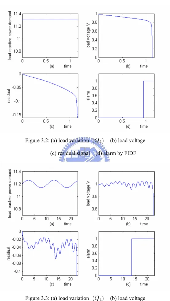
(45) Figure 3.2: (a) load variation (Q 1). (b) load voltage. (c) residual signal (d) alarm by FIDF. Figure 3.3: (a) load variation (Q 1). (b) load voltage. (c) residual signal (d) alarm by FIDF. ３５.

(46) Figure 3.4: (a) load variation (Q 1). (b) load voltage. (c) residual signal (d) alarm by FIDF. Figure 3.5: (a) load variation (Q 1). (b) load voltage. (c) residual signal (d) alarm by FIDF. ３６.

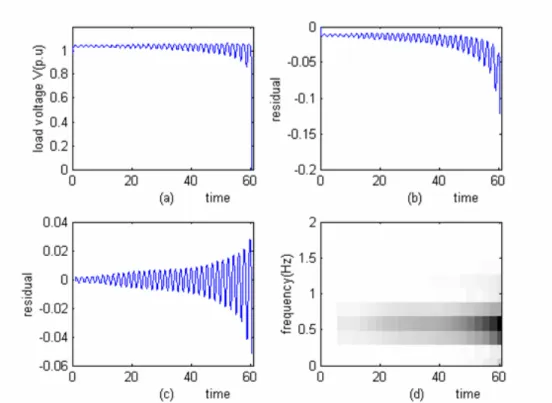
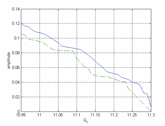
(47) 3.4. Results of Signal Analysis. In addition to FIDF detection as discussed above, it is found from simulation that, when voltage collapse is about to happen for possible Q 1 , the residual signals appear to exhibit oscillation with growing amplitude and almost the same frequency. As such, it enables us to monitor the amplitude of such a frequency to help judge the occurrence of voltage collapse. An example is shown in Figure 3.6, where the load voltage and residual signal for Q 1 ñ 11.1 are given in Figures 3.6(a) and (b), respectively. To avoid the influence of DC part, an averaged signal from the residual by the formula (3.22) below. s a(n) = s(n) à L1. Pn. k= nàL+1. s(k), L = 100. (3.22). and its spectrogram with sampling frequency f s = 100Hz are described in Figures 3.6(c) and (d), respectively. The oscillating frequency to be monitored is observed from Figure 3.6(d) to have f≈0.59Hz . The amplitude of the monitored frequency for the last 1024 points FFT before the occurrence of collapse versus Q 1 is shown by the solid-line of Figure 3.7. To facilitate the detection using the monitored frequency, the threshold values for different Q 1 are defined to be the amplitude of the monitored frequency 5 seconds ahead of voltage collapse, which are indicated by the dashed-line of Figure 3.7. Note that, the oscillating times before collapse are less than 5 seconds near the value of Q 1 = 11.3 . With the definitions of threshold values, the voltage collapse for Q 1 = 11.1 is shown able to be successfully detected using both methods, as indicated in Figures 3.8(b) and (d). The alarm for the second method is fired around t = 55 , which is near 5 seconds ahead of the collapse as desired. Finally, Figure 3.9 demonstrates the detection result for varying load using the threshold which is determined by the second method. Clearly, the alarm is also. ３７.

(48) fired nearly 5 seconds ahead of the occurrence of voltage collapse. Finally, we consider the situation of a 5% load variation about the operating point. Figure 3.10 shows the detection result. It is clear that the alarm is fired nearly 5 seconds ahead of the occurrence of voltage collapse as our desire. From these simulations, it is noted that the voltage collapse can be successfully detected before it occurs. By properly adjusting the threshold for generating the alarm signal, the FIDF may provide a precursor of avoiding undesirable effects of these unstable behaviors.. Figure 3.6: (a) Voltage response for Q 1 ñ 11.1 (b) residual signal (c) residual signal after averaging (d) spectrogram. ３８.

(49) Figure 3.7: Amplitude of the monitored frequency versus Q 1. Figure 3.8: (a) residual signal for Q 1 ñ 11.1. (b) alarm by FIDF (c) amplitude of. the monitored frequency (d) alarm by monitored frequency. ３９.

(50) Figure 3.9: (a) load variation (b) residual signal (c) amplitude of the monitored frequency (d) alarm by monitored frequency. Figure 3.10: (a) load variation (b) residual signal (c) amplitude of the monitored frequency (d) alarm by monitored frequency ４０.

(51) CHAPTER 4 Voltage Regulation of the Electric Power Systems. In this chapter, we add an extra tap changer parallel to the nonlinear load to Dobson and Chiang's power system model for the purpose of voltage regulation. In Section 4.1, we derive the dynamic equations of the power system with tap changer. Then, we will apply Variable Structure Control design scheme to adjust the tap changer ratio to achieve voltage regulation for this model. In Section 4.2, we propose a parameter estimator as the load monitor to provide the load variation of the power system. In Section 4.3, we combine the designs of VSC voltage controller and load estimator to design an adaptive control system.. 4.1 4.1.1. Variable Structure Controller Design Controlled Power System Model. In this section, we add a voltage controller – tap changer to the original power. ４１.

(52) system model. Here, we use the tap changer ratio as the control signal for the electric power system. We will utilize tap changer to regulate the voltage of the electric power system. After adding a voltage controller – tap changer to the original power system model. The controlled model is shown as in Figure 4.1.. Figure 4.1: The power system model with tap changer The original dynamical equations for the electric power system can be written as follow :. îçm = ω. (4.1). Mωç = à d mω + P m + n1 E mY mV sin (î à î m à ò m). + E 2mY m sin ò m. (4.2). K qwîç = à K qv2V 2 à K qvV + Q (î m, î, V) à Q 0 à Q 1. (4.3). TK qwK pvVç = K pwK qv2V 2 + (K pwK qv à K qwK pv) V + K qw (P (î m, î, V) à P 0 à P 1) à K pw (Q (î m, î, V) à Q 0 à Q 1) where. ４２. (4.4).

(53) Q(î m, î, V) = E 00Y00 V cos (î + ò 0 ) + 1n E mYmV cos (î à î m + ò m) ð ñ à Y00 cos ò 00 + n12 Y cos ò m V 2 m. (4.5). P(î m, î, V) = à E 00Y00V sin (î + ò 0) à 1n E mYmV sin (î à î m + ò m) ð ñ à Y00 sin ò 00 + n12 Y sin ò m V 2 m. (4.6). The system parameters we take are the same as those in the Section 3.1.. Let x 1 = î m, x 2 = ω, x 3 = î, x 4 = V . Then, Eqs. (4.1)-(4.4) can be written as :. xç1 = x 2. à áá xç2 = 3.33333 (0.56422 à 0.05x 2 + 5x 4nà1 sin (0.08727 à x 1 + x 3). xç3 = à 33.33333 (à 1.3 à Q1 + 2.8x4 à x24(10.02389 + 4.98097nà2) à áá + 20x 4 cos (0.08727 à x 3) + 5x 4n à1 cos (0.08727 + x 1 à x 3). à à xç4 = à 13.0719 à 1.111x4 + 0.84x24 à 0.4 à 1.3 à Q 1 à x24 ( 7.92389 + 4.98097n à2) + 20x 4 cos (0.08727 à x 3) + 5x 4n à1 cos(0.08727. à + x 1 à x 3)) à 0.03 à 0.6 + x 24(à 1.74311 à 0.43578nà2). + 20x 4 sin(0.08727 à x 3) + 5x 4n à1 sin (0.08727 + x 1 à x 3))). ４３.

(54) 1. For convenience, we let u = n , and expand the above equations. Then the state equations become :. (4.7). xç1 = x 2 â ã xç2 = 1.88073 à 0.16667x 2 + 16.66667x 4 sin(0.0827 à x 1 + x 3) u. (4.8). xç3 = 43.33333 à 93.33333x 4 + 334.12967x 24 à 666.66667x 4 cos(0.08727 â ã à x3) + 33.33333Q1 à 166.66667x4 cos(0.08727 + x1 à x3) u. + 166.03245x24u2. (4.9). xç4 = à 7.03268 + 14.52288x 4 à 53.09608x 24 + (104.5752 cos(0.08727 à x 3). â + 7.84314 sin(0.08727 à x3))x4 à 5.22876Q1 + 26.1438x4. ã â cos(0.08727 + x 1 à x 3) + 1.96079x 4 sin(0.08727 + x 1 à x 3) u. à 26.21518x 24u 2. (4.10). Here, we choose the load voltage as the system output. y = x4. 4.1.2. (4.11). Controller Design. To achieve the main goal – voltage regulation, in the following, we will employ Variable Structure Control (VSC) technique to design controller. As recalled in Chapter 2, it is known that the VSC design procedure consists of two main steps. The first step is to choose a sliding surface, which is a function of system state and desired trajectory. The second step is to design a proper controller to guarantee the state reaching the sliding surface in a finite time and sliding toward the desired trajectory.. ４４.

(55) The power system has the form. xç 4 = f(x) + g 1(x)u + g 2(x)u 2. (4.12). y = x4. (4.13). Suppose x 4d(t) is the desired trajectory. Define the error. e(t) = x 4(t) à x 4d(t). (4.14). For the VSC design first step, we choose the sliding surface to be s(t) = 0 with (4.15). s(t) = e(t) = 0. Clearly, if the system state keeps staying on the sliding surface then the tracking performance can be achieved. That is, e(t) → 0 ñ x 4(t) → x 4d(t) as t → ∞ . The second step of VSC design is to design a control law in the form of. u = u eq + u re. (4.16). To achieve the tracking performance, where u re plays the role of making the error state reach the sliding surface in a finite time and ueq keeps the sliding surface an invariant set and directs the error state to the origin. As mention in Chapter 2, the condition of forcing system state staying on sliding surface can be written as (4.17). sç(t) = 0. By solving the above equation formally for the control input, we can obtain the equivalent control, ueq that would maintain sç = 0 . Consider the system (4.12), the equivalent control can be chosen as. u eq = h(x). (4.18). which h(x) would satisfy. sç(t) = xç 4 à xç 4d. = f(x) + g 1(x)h(x) + g 2(x)h(x) 2 à xç 4d (4.19). =0 For voltage regulation, x 4d is constant, then xç 4d = 0 . ４５.

(56) From (4.12) ~ (4.17), we can obtain. sç(t) = xç 4. = f(x) + g 1(x)(u eq + u re) + g 2(x)(u eq + u re). 2. 2. = f(x) + g 1(x)u eq + g 2(x)(u eq) + g 1(x)u re + 2g 2(x)u equ re + g 2(x)(u re) 2 = [g 1(x) + 2g 2(x)h(x)]u re + g 2(u re) 2. (4.20). From (4.18), we have. s(t)sç(t) = s(t) á [(g 1(x) + 2g 2(x)h(x))u re + g 2(u re) 2]. (4.21). In order to satisfy the sliding condition, we impose the following assumption: Assumption 1 : During the control period, g 1(x) + 2g 2(x)h(x)6=0 .. From assumption 1, we select àñ u re = g1(x)+2g sgn(s) 2(x)h(x). (4.22). where sgn(á ) is the sign function, and ñ is a positive number. It is note that the discontinuity of sign function will cause chattering in the close-loop system. In practice, the sign function sgn(s) is often replace by the saturation function sat(s) where. sat(x) = x ,. if |x| ô 1. sat(x) = sgn(x) ,. if |x| õ 1. (4.23). In order to verify that the control law can satisfy the sliding condition (2.24). We will discuss following possible cases :. ４６.

(57) A. for g 2(x) < 0 (1) s > 0 , we have. ssç = à ñ |s| + s á g 2(x)(u re) 2. < à ñ |s| , for any given ñ (2) s < 0 , we have. ssç = à ñ |s| + s á g 2(x)(u re) 2 ság (x). = à ñ |s| + (g (x)+2g2 (x)h(x)) 2 á ñ2 1. 2. To guarantee the sliding condition, we impose the next assumption : g 2(x). Assumption 2 : (g 1(x)+2g 2(x)h(x)) 2 is bounded. Then we have, ság (x). ssç = à ñ |s| + (g (x)+2g2 (x)h(x)) 2 á ñ2 1. 2. < à kñ |s| , 0 < k < 1 ⇒ñ<. (kà1)á(g 1(x)+2g 2(x)h(x)) 2 g 2(x). B. for g 2(x) > 0 (1) s > 0 ság (x). ssç = à ñ |s| + (g (x)+2g2 (x)h(x)) 2 á ñ2 1. from assumption 2, we have for. ñ<. 2. ssç < à kñ |s| , 0 < k < 1. (1àk)á(g 1(x)+2g 2(x)h(x)) 2 g 2(x). (2) s < 0 , we have. ssç = à ñ |s| + s á g 2(x)(u re) 2. < à ñ |s| , for any given ñ ４７.