離子幫浦的隨機熱力學

國

立

交

通

大

學

物理研究所

碩

士

論

文

離子幫浦的隨機熱力學

Stochastic Thermodynamics in Ion Pumps

研 究 生：張朝昇

指導教授：張正宏 教授

I 誌謝 ... II Abstract ... III 摘要 ... IV Content ... 1 1 Stochastic thermodynamics... 1

1.1 Integral fluctuation theorem and detailed fluctuation theorem ... 2

The detailed balance condition and the static detailed balance condition... 3

The derivation of the IFT for a master equation ... 3

1.2 Stochastic entropy along a single trajectory ... 7

2 An experiment test and simulation for two-state system ... 12

2.1 Experimental test for entropy production of a two-level system ... 12

2.2 Reproduction of the experiment by simulation ... 14

2.3 Improvements in simulation ... 20

2.3.1 Consideration of the ensemble average of states ... 20

2.3.2 Estimation for quantity of statistics ... 24

2.4 Brief conclusion ... 31

3 A simulation for entropy production for four-state system ... 32

3.1 The four-state system for ion pumps ... 32

3.2 The simulation for four-state system ... 32

3.2.1 Time-dependent detailed balance condition without net flow ... 33

3.2.2 Static detailed balance condition with net flow ... 35

3.2.3 Non-detailed balance condition without time-dependent driving ... 39

3.2.4 Non-detailed balance condition with time-dependent driving ... 42

3.3 Brief conclusion ... 49

Conclusions and Future Works ... 51

II

誌 謝

III

Abstract

In chapter 1, we give a brief introduction to stochastic thermodynamics, and then make use of the notion of time-reversal to derive the integral fluctuation theorem (IFT) as a mathematical result for general discrete-state system governed by a master equation. Next, applying the definition [1] of entropy along a single stochastic trajectory, we get the integral fluctuation theorem (IFT) for stochastic thermodynamics.

In chapter 2, we first sketch the two-level experiment with a single defect center in diamond periodically excited by a laser [2], which verified the validity of the definition of entropy along a stochastic trajectory, as well as integral fluctuation theorem (IFT) and detailed fluctuation theorems (DFT) in a two-state system. Then, we develop a simulation for the Markovian process in this discrete system, to confirm the experimental observation. Next, we improve the experimental conditions in the simulation and get more information than the experiments about how the data collected converge to the IFT and DFT.

In chapter 3, we apply the similar simulation to the four-state system of ion pumps and discuss stochastic thermodynamics under different conditions, such as different external protocols and whether obey detailed balance condition.

IV

摘 要

在第一章，我們為隨機熱力學(Stochastic Thermodynamics)做簡短的介紹， 並 利 用 時 間 反 轉 的 方 法 證 明 離 散 系 統 (discrete system) 中 的 Integral Fluctuation Theorem (IFT)。IFT 原本只是數學上的結果，但如果我們引進單 一路徑的 entropy 定義 [1]，我們就可以得到隨機熱力學中的 IFT。

在第二章，我們介紹一個二階系統的實驗 [2]，這是一個在鑽石中受週期雷 射激發的單一缺陷。一個缺陷會有基態和激發態兩種狀態，而對於很多個缺陷則 可以用 master equation 來描述它們所處狀態的濃度。透過這個實驗，可以檢驗 二階系統中單一路徑的 entropy 定義、IFT，以及 Detailed Fluctuation Theorem (DFT) 的正確性。接著我們用程式模擬這個二階系統和實驗結果，並進一步地改 善實驗條件，使得結果更接近 IFT 和 DFT 的理論值。

在第三章，我們討論各種不同條件下的鈉鉀離子幫浦的隨機熱力學，像是外 加不同的外場，以及系統是不是符合 detailed balance condition. 我們先將 其簡化成四階系統，並應用第二章的模擬方法去討論各種條件下的情形。

1

Content

1 Stochastic thermodynamics

Stochastic thermodynamics provides a conceptual framework for describing a large class of soft and bio matter systems under well specified but still fairly general non-equilibrium conditions. Typical examples comprise colloidal particles driven by time-dependent laser traps and polymers or biomolecules like RNA, DNA or proteins manipulated by optical tweezers.

The experiment [3] of the stretching of RNA on a nano-scale is one of the typical experiments for stochastic thermodynamics. Therein, two conceptual issues must be faced if one wants to use the same macroscopic notions to describe such an experiment. First, how should work, exchanged heat and internal energy be defined on this scale? Second, these quantities do not acquire sharp values but rather lead to distributions, as shown in Figure 1-1. The occurrence of negative value of the dissipated work is typical for such distributions.

Figure 1-1

Measured distributions for dissipative work during RNA stretching. The three

panels correspond to different extensions whereas the color refers to different pulling speeds [3].

2

on different kinds of distributions and relate them to quantities in classical thermodynamics. The key interested issues include IFT, DFT, generalized Einstein relations, and generalized fluctuation dissipation theorem [4] etc.

1.1 Integral fluctuation theorem and detailed fluctuation theorem

The second law of classical thermodynamics states that the entropy keeps increasing over time in a closed system. But in some particular situations one might doubt that whether entropy could decrease rather than increase in short time, and violate the second law of classical thermodynamics. This idea has ever noticed in nano-technology but hasn’t caught much attention until 1993, when quantitative description of a violation of the second law in finite systems was first given by the fluctuation theorem of Evans et al. [5]. This fluctuation relation in computer simulations of sheared liquids is a surprisingly simple relation between the probability to observe entropy generation and that to observe the corresponding entropy consumption.

To show how the IFT arises, we give an example as follows. Imagined that there are two rooms next to each other with a door between, and the room A is full of air molecules while the other room B is totally empty. After the door is opened, some molecules in room A start moving and end at somewhere in room B along certain trajectories. According to the time reversibility of Newtonian dynamics, the molecules just mentioned may also move from the ending places in room B to the original places in room A along the same but reversed trajectories. However, this phenomenon seldom occurs according our experiences, or the second law of classical thermodynamics. Nevertheless, in a tiny system and short time, the phenomenon would occur with a larger probability compared to a macroscopic system. In fact, the IFT and the DFT are the theorems which are capable of revealing the relations

3

between the forward and the reversed trajectories.

The detailed balance condition and the static detailed balance condition

In equilibrium, the stationary distribution necessarily obeys the detailed balance condition

(1-1)

where m is the state next to n. In other words, the detailed balance condition is the definition of equilibrium. However, the cases in which we are interested are usually far from equilibrium, so there is another version of the detailed balance condition in nonequilibrium systems.

For a fixed in a nonequilibrium system, if the stationary distribution obeys the detailed balance condition (1-1), we call this condition the static detailed balance condition. In other words, for a fixed time, there exists an “expected equilibrium state” but this state cannot ever be reached due to the external protocol.

Based on the static detailed balance condition, the DFT can be derived [6] and is given by

(1-2)

Where is the probability for the trajectories to measure the total entropy production equal to , whereas is that to measure the total entropy production equal to .

The derivation of the IFT for a master equation

The recent research for stochastic thermodynamics has involved in two approaches: the diffusive system governed by the Langevin equation and the discrete-state system governed by a master equation. This thesis is focused on the

4

latter.

Below we will prove the IFT for the discrete-state system governed by a master equation. First, we consider a stochastic dynamics on an arbitrary set of states and the dynamics is governed by a master equation, which reads

(1-3)

where is the probability to be at state at time and only the jumps to neighbor states are allowed. represents the transition rate from state to the neighbor state and depends on an external time-dependent protocol .

Figure 1-2

(a) A network with states connected by transition rates and (b) a

trajectory jumping at the time sequence , with .

Then we apply the fluctuation theorem to stochastic trajectories . The trajectory is obtained by starting the system in a stationary state obeying detailed balance for the fixed and then driving it according to some protocol from . Below we will prove [6] that the trajectories obey the integral fluctuation theorem

_(1-4)

5

where is the ratio of the probability which will be defined soon later, and the average is taken over infinitely many trajectories.

We assume that for a fixed the system is in a stationary state obeying the detailed balance (1-1). Therefore, the probability for a trajectory starting at state , jumping to at , jumping to at

, , finally jumping to at and staying there till time , is given by (1-5) On the other hand, the probability for the reversed trajectory occurring under the reversed protocol is given by

(1-6)

6 Figure 1-3

An example of the reversed trajectory [red line] and the reversed protocol compared to the ordinary ones [blue line].

The crucial quantity is the ratio

(1-7)

where the last term follows by the cancellation of the exponential integral terms in

(1-5) and (1-6). Then the IFT can be proved by the normalization condition in which

the sum of over all possible trajectories is equal to one. Before summing over trajectories, we multiply (1-7) by . It reads

_{. (1-8)}

Then summing over the possible trajectories

_(1-9)

Finally, we change the notation into and thus have

_(1-10)

So far we have proved the IFT (1-10) for stochastic trajectories by introducing the reversed trajectory and the stochastic quantity . This

0 0 n t t (a) (b)

7

result is a mathematical result and seems not to be associated with thermodynamics. Nevertheless, the meaning of the IFT would become transparent after introducing the stochastic entropy along a single trajectory in the next section.

1.2 Stochastic entropy along a single trajectory

Entropy might be considered as an ensemble property and therefore seems not to be applicable to a single trajectory. However, the previous research for so-called fluctuation theorems generally [9] relates the probability of entropy generating trajectories to that of entropy annihilating trajectories. So it obviously requires a definition of entropy on the level of a single trajectory. Therefore, the definition of entropy production along a single stochastic trajectory is introduced through the diffusive system with a particle in overdamped motion [1], then generalized to the discrete-system governed by a master equation.

At first, from the common definition of a nonequilibrium Gibbs entropy [8] (1-11) the suggested definition for trajectory-dependent entropy of the system for a Brownian particle is given by

, (1-12)

where the probability is obtained by solving the Fokker-Planck equation (1-13) Similarly, the definition of trajectory-dependent system entropy for the probability derived from a master equation is given by

ln (1-14)

8

change is derived from the equations of motions [1]. Therefore, the similar derivation is also applied to the discrete-state system. The equation of motion for the system entropy becomes

(1-15)

The first term on the right-hand side contributes along the time intervals during which the system remains in the same states; to more explicitly, the system is at the same state during the time intervals whereas the time-dependent protocol and the corresponding probability of the state keep changing, and thus it results in the part of due to the change of the protocol. On the other hand, the second term arises from the jumps at ; to more explicitly, the time-dependent protocol and the corresponding probability of the state remain the same at when jumps occur whereas the system change the states, and thus it results in the other part of due to the change of states.

Now we split up the right-hand side of (1-15) into a total entropy production and a medium entropy production as follows.

(1-16) and _(1-17)

where is the transition rate for forward jump and is that for backward jump. Besides, the balance holds.

Although the choice of seems to be arbitrary, there are two facts which motivate this choice. First, we would observe the ensemble properties of entropy by

9

taking average over trajectories, so we need the probability for a jump occurring at from to , which is . Hence, these entropy become

(1-18) _(1-19) and (1-20)

such that the balance holds. Besides, the ensemble of total entropy production in (1-20) is consistent with the macroscopic entropy (1-11)

and thus obeying the second law of classical thermodynamics. Second, with this choice of in (1-17), the total entropy production fulfills the IFT, which we will show below.

With the definitions for entropy along a single stochastic trajectory (1-15) (1-16)

(1-17), the meaning of the IFT (1-10) becomes transparent, which is derived from the

discrete-state system governed by a master equation. At first, we recall the stochastic quantity from (1-7) (1-21) Then we split up the right hand side of (1-21) into the contribution of and , according to the interpretation of (1-15) and (1-17). That is,

10 (1-23) (1-24)

where we have used the definition . Then finally,

(1-25)

where is the first term and is the second term in (1-24).

So far we proved that the stochastic quantity defined as is exactly the total entropy production in the discrete-state system governed by a master equation.

Therefore, the integral fluctuation theorem becomes

_(1-26)

As an immediate consequence of (1-26), one can derive a formula

according to Jensen’s inequality . This result is consistent with the second law of classical thermodynamics and gives an a posteriori support to the entropy definition.

So far, the main result is proved but there is still one thing which has to be referred. Although we start the derivation for the IFT from the stationary distribution and obeying detailed balance for a fixed , the choice for the initial and final distribution, in fact, are not uniquely selected. As a mathematical result, the IFT is truly universal which is valid for any external protocol, any initial conditions, and any trajectory length, so there are infinitely many choices of initial and final distribution. Nevertheless, the most intuitive and physically meaningful choice might be and , which the former stands for stationary state with

11

, and the latter is the state which has reached the static state after a long time. Notice that the probability in a static state discussed in this thesis might still oscillate but doesn’t ascend or descend on average over time.

In the later sections, this choice of and is applied mostly to our discussion.

12

2 An experiment test and simulation for two-state system

2.1 Experimental test for entropy production of a two-level system

To verify the fluctuation theorem in a nonthermal system with time-dependent rates, an experiment of a two-level system is demonstrated [2]. The device with a single defect center in natural IIa-type diamond (Drukker) is excited by a red and a green laser simultaneously and can be considered as an effective two-level system with a dark and a bright state, such that

_,

where and are determined by the green and red lasers respectively.

This system is driven out of the initial equilibrium by modulating the intensity of the green laser with a sinusoidal protocol with modulation period . This leads to the time-dependent rate

(2-1)

with

, (2-2)

where 0 < < 1 is the strength of the modulation. The intensity of the red laser is constant and therefore . Therefore, the master equation for the time-dependent probability and of this two-level system then reads

(2-3)

where the and represent the probabilities for the system being at state 0 and 1 stays, respectively. Once the probability distribution of the system is given, a dimensionless, nonequilibrium entropy for driven systems on the level of a single

13

stochastic trajectory has been defined [1] as

, (2-4)

where the measured probability at state at is determined by the master equation.

Figure 2-1 [2]

Figure 2-1 (a) shows the protocol together with the probability to

dwell in the bright state or state one. The step function Figure 2-1 (b) displays a sample binary trajectory jumping between the two states. In Figure 2-1 (c), the protocol gives the evolution of the entropy of the system according to (2-4). The curve consists of smooth part and the jump part. The smooth part is due to the time-dependent protocol at the same state; the jump part is due to the contribution between the two states, where and are the probabilities of the states immediately before and after the jump respectively.

Besides the entropy of the system itself, energy exchange and dissipation lead, in general, to a change in medium entropy. For an athermal system such as a discrete state system, this change in medium entropy cannot be inferred from the

14

exchanged heat. Rather it has to be defined through the rate constants, and is given by

(2-5)

for a jump from state to state with instantaneous rate ( being the backward rate). In this case it becomes for a jump 1→0 and for a jump 0→1. As demonstrated in Figure 2-1 (d), the medium entropy changes only when the system jumps, thus balancing to some degree the change of .

One of the fundamental consequences of the definition of stochastic entropy is the fact that besides entropy producing trajectories, entropy annihilating trajectories also exist; see Figure 2-1 (e) and (f), respectively. However, in accordance with physical intuition, the latter become less likely for longer trajectories or increased system size. In fact, entropy annihilating trajectories not only exist, they are essential to satisfy the IFT

exp (2-6)

This theorem states that the non-uniform average of the total entropy change over infinite trajectories becomes unity for any trajectory length and any driving protocol. Moreover, trajectories with may seldom occur but are exponentially weighted and thus give a contribution substantially to the left hand side of (2-6).

2.2 Reproduction of the experiment by simulation

The validity of the definition of stochastic entropy for a single trajectory and the corresponding IFT is in principle verified by the experiment of two-state system stated above. Nevertheless, restricted by the intrinsic limitation of experiments such as the amount of data, the resolution of instruments, and etc., there are still some

15

conditions which cannot be verified thoroughly.

The resolution of the detectors in the experiment is 1ms and therefore the measurable shortest time interval between two jumps must be 1ms or longer. Nevertheless, is the resolution short enough to detect the fastest jumps between states? How would the measured transition rates be affected if the resolution is longer or shorter?

Besides the resolution, the amount of the realizations is also a limit of experiments. Although the IFT is valid for summing over infinite number of trajectories, the tests with only 2000 trajectories in the experiment seem to be sufficient for IFT. Nevertheless, is it enough for thousands of trajectories all the time? What if the conditions such as the external protocol or the trajectory length change? The IFT is generally valid but is there any experimental condition beyond the feasibility?

Therefore, as an a priori tool, a simulation based on the conditions of the experiment stated above is developed to recheck the validity of the definition of stochastic entropy for a single trajectory and the corresponding IFT, and furthermore examine another conditions for a two-state system.

The simulation is developed on the idea of throwing a stochastic die sequentially with the same time interval. The first step of the simulation is to create a single trajectory and then we can get an ensemble of trajectories. Assumed that the system is initially at state-one, then a die is thrown after a period of time to decide whether the system will stay still or jump to the other state, that is state-two. If the side of “jump” is on the top, the system will jump to the other state instantly without any hesitate and wait for the next chance to throw a die. Whether the system stood still or jumped to

16

the other state this time, the next chance to throw a die is totally independent. That is, the process is Markovian.

The method of the simulation

The probability of jumping depends on the product of transition rate and the given time interval , that is

. (2-7)

where is the probability jumping from -state to -state. For example, if the given interval is 1ms and the transition rate from state-1 to state-2 at a certain time is 500(1/s), then the system has probability to jump from 1 to 2 at that moment. Note that the jump probability is different from the state

probability derived from a master equation. The latter means the probability which the system should be found in state- over averaging many trajectories and thus an ensemble quantity. On the other hand, although the former also means probability, it is a quantity for each time to throw a die for each trajectory. Besides, the time interval is arbitrary and decides the probability to jump. The shorter the , the less probable the system would jump and vice versa. Be careful to choose a suitable so that the probability to jump would not be larger than one at any time over the total process, or it would be ambiguous otherwise.

With the transition rates, initial probability distribution for stationary states, and the definitions for system entropy Eq. (2-4) and medium entropy Eq. (2-5), a set of

Figure 2-2 (a)(b)(c) and Figure 2-3 (a)(b) for a single trajectory similar to the two-state

17 Figure 2-2

Entropy production in the two-state system with a single defect center in diamond, with parameters , , , and for a single trajectory over 4 periods. (a) shows the protocol [solid blue line] together with the probability [dashed green line] to dwell in the state one. (b)

Single trajectory [solid blue line] and probability of state-one [dashed green line]. (c) Evolution of the system entropy [black dots]. The curve is much smoother than that in Figure 2-1 (c) when the system is at the same state because Figure 2-1 (c)

is experimental measurement. (d) Entropy change of the medium, where only jumps contribute to the entropy change.

0.02 0.04 0.06 0.08 0.1 0.12 0.14 0.16 0.18 0.4 0.6 0.8 1 0 0.02 0.04 0.06 0.08 0.1 0.12 0.14 0.16 0.18 0.2 0 0.5 1 0.02 0.04 0.06 0.08 0.1 0.12 0.14 0.16 0.18 50 100 0 0.02 0.04 0.06 0.08 0.1 0.12 0.14 0.16 0.18 0.20.4 0.6 0.8 0 0.5 1 (a) (b) (c) (d)

18 Figure 2-3

Two examples of the change of system entropy [solid black line] and medium entropy [dashed red line]. The dashed blue lines indicate the original value of the entropy. The change of system entropy just fluctuates around zero without net average entropy production, whereas in (a) contributes positive change of entropy and thus an entropy producing trajectory and (b) contributes negative change of entropy and thus an entropy annihilating trajectory.

After creating a single trajectory, an ensemble of trajectories can also be created to check the validity of IFT. Figure 2-4 is a set of the histograms of entropy change of

(a) system, (b) medium and (c) total entropy production taken from 2000 trajectories with the same condition in the two-state experiment Figure 2-1 (g)(h)(i).

0 0.1 0.2 0.3 0.4 0.5 0.6 0.7 0.8 0.9 1 0 1 2 3 4 0 0.1 0.2 0.3 0.4 0.5 0.6 0.7 0.8 0.9 1 -1 0 1 (a) (b) t/s ,

19 Figure 2-4

Histograms taken from 2000 trajectories of the (a) system, the (b) medium, and the

(c) total entropy change. The system entropy shows four peaks corresponding to four possibilities for the trajectory to start and end (0→1, 1→0, 0→0, and 1→1). The distribution (c) of the total entropy change has the mean and width ; on this scale it differs only slightly from the distribution of the medium

entropy change (b).

In Figure 2-5, the calculations of IFT taken from 2000 trajectories for period

from 1 to 20 are demonstrated. Note that each period is calculated 5 times to examine the deviation of the outcome of IFT. With increased length, a deviation of IFT becomes observable. This deviation is due to the requirement for more realizations as the mean value of the entropy increases and the deviation can be corrected in the latter section. -1 -0.5 0 0.5 1 0 100 200 300 400 500 600 700  system entropy nu m be r of t ra je ct or ie s -5 0 5 0 50 100 150 200 250  medium entropy -5 0 5 0 50 100 150 200 250  total entropy (b) (c) (a)

20 Figure 2-5

The mean over 2000 trajectories for each period with the modulation

depth .

2.3 Improvements in simulation

2.3.1 Consideration of the ensemble average of states

So far we have reproduced the main results of the two-state experiment [2], and the next step is to improve the experimental conditions. First, we determine the probability for the system being at the state-one by taking average over stochastic trajectories and derive the ensemble average of states for state-one, and we call this quantity . means the probability which the system is at state-one from the viewpoint of single trajectories, whereas is derived from the master equation.

The interpretation of has many advantages which would be seen soon later. The most important one is to check the idea of throwing a die and the correctness of the simulation. If there is something wrong, the curve of would be totally different from the curve of probability for the corresponding state.

0 2 4 6 8 10 12 14 16 18 20 0.7 0.8 0.9 1 1.1 1.2

Trajectory length (# of periods)

21

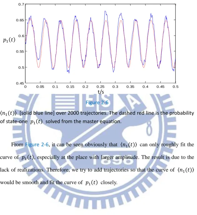
Figure 2-6 shows averaged from 2000 trajectories with the condition of the

two-state experiment.

Figure 2-6

[solid blue line] over 2000 trajectories. The dashed red line is the probability of state-one solved from the master equation.

From Figure 2-6, it can be seen obviously that can only roughly fit the

curve of , especially at the place with larger amplitude. The result is due to the lack of realizations. Therefore, we try to add trajectories so that the curve of would be smooth and fit the curve of closely.

0 0.05 0.1 0.15 0.2 0.25 0.3 0.35 0.4 0.45 0.5 0.45 0.5 0.55 0.6 0.65 0.7 t/s

22 Figure 2-7

The mean [solid blue line] of state-one over 100,000 trajectories compared to the probability of state-one [dashed red line].

With increased realizations, it seems the curve of fit that of more closely and IFT is also more accurate (Figure 2-8) rather than the results in Figure 2-5.

Figure 2-8

The mean over 100,000 trajectories for each period with the

modulation depth and resolution . IFT is calculated 5 times for each period in order to examine the deviation.

0 0.05 0.1 0.15 0.2 0.25 0.3 0.35 0.4 0.45 0.5 0.45 0.5 0.55 0.6 0.65 0.7 0 2 4 6 8 10 12 14 16 18 20 0.95 0.96 0.97 0.98 0.99 1 1.01 1.02 1.03 1.04 1.05 t/s

Length of trajectories (# of periods)

23

Although IFT becomes more accurate after adding more realizations and its validity is also verified in principle, there is something needed to examine more carefully. If we zoom into just one period in Figure 2-7 (Figure 2-9 (a)), one can find there is a constant phase delay of compared to that of . This is due to the low resolution. Although it doesn’t affect the validity of IFT, it implies that the external protocol we are studying is a little different from the real one and this difference would result in a little deviation in the mean . Figure 2-9 shows the

figures with different resolution and the corresponding . Because the curve in

Figure 2-9 (C) fits most closely, it might approach most the “real” value of

.

Figure 2-9

The blue lines represent and the red lines represent over 100,000 trajectories, respectively. (a), (b) and (c) are intercepted from trajectories of 20 periods with different resolution 5ms, 1ms and 0.1ms respectively.

0.56 0.58 0.6 0.5 0.55 0.6 0.65 0.46 0.48 0.5 0.5 0.55 0.6 0.65 0.36 0.38 0.4 0.5 0.55 0.6 0.65 (b) (a) t/s (c) Resolution=5ms =1.789 t/s Resolution=1ms =1.743 t/s Resolution=0.1ms =1.735

24

2.3.2 Estimation for quantity of statistics

With only 2000 trajectories and under suitable experimental conditions, such as trajectory length, resolution, modulation depth etc., it seems that IFT works well in principle (deviation < 20%, Figure 2-5). In the simulation, IFT is even confirmed with higher accuracy (deviation < 5%, Figure 2-8) when the number of trajectories is increased to 100,000. Nevertheless, is this number large enough for other conditions? To show this concern is necessary, we take longer observation time. Figure 2-10

demonstrates that the deviation is increased with the number of period. The example

Figure 2-10 (a) has a point separated far from others, which seems to be absurd at first

glance. But in fact, this extreme case appears typically.

0 10 20 30 40 50 60 70 80 90 100 0 0.5 1 1.5 2 2.5 3 3.5 4 (a)

25 Figure 2-10

The mean over 100,000 trajectories for each period with the

modulation depth and resolution . Same as the former examples, IFT is calculated 5 times for each period in order to examine the deviation. Notice that there is a point at the upper right corner. Note the red dashed rectangle is just

Figure 2-8 and Figure 2-10 (b) is the magnified view of (a) omitting the point at the

upper right corner.

The result in Figure 2-10 is due to the structure of the non-uniform average . Because the entropy annihilating trajectories may occur seldom but are exponentially weighted, they contribute substantially to the left hand side of IFT. To keep , each of entropy annihilating trajectories needs a large quantity of entropy producing trajectories to balance. Therefore, the variation on the number of entropy annihilating trajectories would affect the results of IFT enormously, especially when the number of annihilating trajectories is small. With increased observation time, the mean of total entropy production shifts in a positive direction and spreads outwards in both directions (Figure 2-11 and Figure 2-12). The number of annihilating trajectories also decreases, and it leads to the larger deviation of IFT. In most situations, a large number of entropy producing trajectories

0 10 20 30 40 50 60 70 80 90 100 0.5 0.6 0.7 0.8 0.9 1 1.1 1.2 1.3 1.4 1.5 (b)

Length of trajectories (# of periods)

26

lacks sufficient number of annihilating ones to balance, which brings about the result of . But sometimes, too many, or even a little more entropy annihilating trajectories are generated, resulting in . This explains

the distribution of in Figure 2-10.

Figure 2-11

Histograms of total entropy production with different periods of (a) 20T, (b)

60T, and (c) 100T, respectively. The mean and the width (two standard

deviations) of are also shown in each figure.

0 100 200 300 0 100 200 300 -10 -5 0 5 10 15 20 25 30 0 100 200 300 (a) (b) (c)

27 Figure 2-12

The mean of total entropy production is proportional to the trajectory

length. It seems surprising at first glance but in fact can be explained easily; because the total process is Markovian, the change of from periods

must be the same as that from and so on.

Except for the rough description from Figure 2-11, the relation between the probability of entropy producing trajectories and entropy annihilating trajectories, in fact, obeys the detailed fluctuation theorem (DFT) [7]

(2-8)

Where is the probability for the trajectories to measure the total entropy production equal to , whereas is that to measure the total entropy production equal to .

This theorem was derived originally for the long time limit in nonequilibrium steady states. However, it even holds as long as the protocol driving the system is periodic and time-symmetric, as well as the probability distribution has relaxed into the corresponding periodically oscillating distribution. In this case, the

10 20 30 40 50 60 70 80 90 100 0 1 2 3 4 5 6 7 8 9 th e m ea n o f to ta l en tr op y pr o d uct io n

the length of a trajectory

Length of trajectories (# of periods)

28

trajectory length is very long and thus dominates . Therefore, DFT is valid in principle and suitable for the estimation.

Figure 2-13

The test diagram of DFT for the data set (i). The red asterisk denotes the mean of total entropy production and the points near have more accuracy

of the DFT. The blank on the right side represents the missing points due to the lack of realizations; some positive entropy production can not correspond to their

negative entropy production .

The dashed line is with slope = 1.

To estimate the trajectory number required to verify IFT, we take an example as follows. Assumed there are two sets of data to verify the IFT of two-state system.

(i) 20 periods and over 100,000 trajectories (j) 40 periods and over 100,000 trajectories.

As shown in Figure 2-10, IFT works very well in the data set (i) but not in the data set (j) and we wonder how large the trajectory number does (j) require to get a satisfactory result as in (i).

0 1 2 3 4 5 6 7 8 9 10 0 1 2 3 4 5 6 7 8 9 10

29

Whether IFT works well depends on whether DFT works well throughout

Figure 2-13. Of course we cannot examine DFT for each , so our method of

estimation is to examine DFT for the most frequency value . The number of trajectories with (with error in the simulation) in (i) is approximately 375 and the corresponding number of trajectories with is estimated to be 64.9 according to DFT but is 66 actually. The little variation doesn’t matter and the number 64.9 of trajectories of is large enough, so that the number of trajectories is also large enough to verify IFT in (i).

Because the trajectory length with decreases exponentially with increased according to DFT, to maintain these rare trajectories to balance

those with , the number of total trajectories also has to be increased exponentially, that is

_(2-9)

Where is the trajectory number with which IFT can be verified satisfactorily in the data set (i); is the required trajectory number in a certain data set (j) to satisfy IFT with the same accuracy as in (i); and are the means of total entropy production in (i) and (j), respectively.

With this estimation, for each trajectory length can be calculated easily

(Figure 2-14). On the other hand, because the total entropy production is

linearly weighted in rather than exponentially weighted, would converge to the stable value without large trajectory number. Applying to the calculations of IFT, corrected and satisfactory results are shown in Figure 2-15.

30 Figure 2-14

The reference 100000 is in the condition with 20 periods and .

With increased length from 20 to 100 periods, is also increased linearly and

it results in the exponentially increased .

Figure 2-15 10 20 30 40 50 60 70 80 90 100 110 0 2 4 6 8 10 12x 10 7 100000 240000 590000 1430000 3430000 8290000 20080000 48630000 117890000 0 10 20 30 40 50 60 70 80 90 100 110 0.6 0.7 0.8 0.9 1 1.1 1.2

Trajectory length (# of periods)

Trajectory length (# of periods)

31

The results of IFT versus the trajectory length over 100000 trajectories ([blue circles] taken from Figure 2-10 (b) omitting the separate point) and over [red asterisks] corrected trajectory number shown in Figure 2-14. Note IFT is calculated five times for each length.

The results of IFT with the corrected numbers of trajectories are obviously more accurate than the original ones. It means this estimation is correct at least in the order of magnitude. Nevertheless, with the longer trajectory length, the results are not as accurate as the result of 20 periods; it means the required number is increased at least exponentially with the mean .

2.4 Brief conclusion

In conclusion, in this chapter a method of simulation is developed to reproduce the experiment of two-state system driven by a sinusoidal protocol. There are three important points in the simulation. The first one is throwing a stochastic die sequentially with the same time interval and then individual stochastic trajectories can be generated. The second one is determining the state probability by taking average over trajectories. This probability of the -state should be the same as that derived from the master equation. This check tests if the given resolution and the trajectory number are sufficient to produce good data under the external protocol. The third point is the estimation of the required trajectory number. According to DFT, we find that the required number to verify IFT at least increases exponentially with the mean , where the mean is linear to the trajectory length.

32

3 A simulation for entropy production for four-state system

3.1 The four-state system for ion pumps

In this chapter, we consider four-state systems with different conditions based on the ion pumps of Na and K-ATPase.

Na, K-ATPase is a molecular motor, whose mechanism of action is shown to be consistent with the flashing ratchet [11]. The enzyme is a transmembrane protein complex, which can pump Na+ and K+ against the concentration gradients across the cell membrane. In a cell the energy required for the active transport is derived from the hydrolysis of ATP (adenosine triphosphate) or from the fluctuation of the transmembrane electric potential [12]. The former cause the violation of detailed balance condition and the latter is the external time-dependent protocol in our simulation for four-state systems.

3.2 The simulation for four-state system

One of the features of the ion-pump system is that, even if the stationary distribution obeys the detailed balance condition for fixed protocol , or the system obeys the static detailed balance condition, the protocol may still drive the system toward a specific direction. That is, there is net flow in the ion-pump system.

In most situations, the concentrations keep flowing to the neighbor states in a specific direction and thus it results in net flow. But there is a special case in which the concentration distribution doesn’t change over time and thus there is no transition flux between the neighbor states, even if the system is subject to a time dependent protocol. Sometimes this condition is called the time-dependent detailed balance.

33

3.2.1 Time-dependent detailed balance condition without net flow

The set of transition rates given below obeys the time-dependent detailed balance condition and contributes no net flow in the ion pump system.

where and the amplitude A is set as 1.

With this set of transition rates, the averaged transition flux between the

states and over one period T is zero, where over one period T reads

(3-1)

Because the time-dependent transition rates between the states are changed simultaneously and proportionally, there is no flux between states and the concentration distribution remains the same.

The main results for 20 periods over 100,000 trajectories are follows.

where is the number of turns of a stochastic trajectory and is the average of over trajectories. Moreover, is equal to the total jumps divided by four. 1 2 3 4

34 Figure 3-1

An example of a single trajectory. (a) The state at which the system stays. (b) The system entropy due to . (c) The system entropy change which

subtracts the initial value of the system entropy from the system entropy, that is, . (d) The change of system entropy due to .

1 2 3 4 1 1.5 2 0 0.5 1 0 0.02 0.04 0.06 0.08 0.1 0.12 -1 -0.5 0 -1 -0.8 -0.6 -0.4 -0.2 0 0.2 0.4 0.6 0.8 1 0 2 4 6 8 10x 10 4

Trajectory length (second) n (a) (b) (a) (c) (d)

35 Figure 3-2

The total entropy production for trajectories is exactly zero (Figure 3-2 (a));

the result can be realized from a single trajectory (Figure 3-1). When the system jumps from to , the system entropy change is ln . On the other hand, the medium entropy change is . And because the

system obeys the time-dependent detailed balance, the equation is always true with time, the medium entropy change becomes

. Therefore, the total entropy production for each

jump of a single trajectory and it results in Figure 3-2 (a).

Because is zero for each trajectory, the IFT and the DFT are fulfilled trivially. Besides, the number of turns of each trajectory is symmetric because the system doesn’t prefer any direction due to the protocol.

3.2.2 Static detailed balance condition with net flow

In general situations of the ion pump, the external time-dependent protocol would drive the system and the concentrations of each state would flow towards the same direction on average over time. Besides, some protocols would drive the system clockwise and another would drive the system counterclockwise because the system

-5 -4 -3 -2 -1 0 1 2 3 4 5 0 2000 4000 6000 8000 10000 12000 14000 (b)

36

itself hasn’t any preference for the protocol.

The set of transition rates given below drives the system clockwise, or in the positive direction.

The main results for 20 periods over 100,000 trajectories are follows.

where and because the system goes in the positive direction.

-10 -5 0 5 10 15 20 0 200 400 600 800 1000 1200 1400 1600 1800 2000 -5 -4 -3 -2 -1 0 1 2 3 4 5 6 7 0 2000 4000 6000 8000 10000 12000 1 2 3 4 (a) (b)

37 Figure 3-3

(a) and (b) are the histograms of and for 20 periods over 100,000

trajectories, and (c) is the test diagram of the DFT with the red asterisk denoting the mean .

The IFT remains valid in this case because the number of entropy annihilating trajectories is large enough to balance the number of entropy producing trajectories.

Figure 3-3 (c) shows the DFT test and the red asterisk denotes the mean . It can

be seen that DFT is accurate if the point representing the trajectory number with is not much far from the mean . Nevertheless, there are many missing

points due to the insufficient number of realizations; the largest value of is 16.5 whereas the smallest one is -7.3, so not each positive entropy production can be compared with its corresponding negative entropy production . The large blank on the right side in Figure 3-3 (c) just indicates this situation

0 2 4 6 8 10 12 14 16 0 2 4 6 8 10 12 14 16 (c)

38

The set of transition rates given below drives the system counterclockwise, or in the negative direction.

The main results for 20 periods over 100,000 trajectories are follows.

where and because the system goes in the negative direction.

-10 -5 0 5 10 15 20 0 200 400 600 800 1000 1200 1400 1600 1800 -8 -7 -6 -5 -4 -3 -2 -1 0 1 2 3 4 5 0 1000 2000 3000 4000 5000 6000 7000 8000 1 2 3 4 (a) (b)

39 Figure 3-4

(a) and (b) are the histograms of and for 20 periods over 100,000

trajectories, and (c) is the test diagram of the DFT with the red asterisk denoting the mean .

The mean of total entropy production is always positive no matter whether the system goes in the positive direction or negative direction; because both the contributions and of , are not oriented to directions and evaluated by (2-5) and due to (2-4). Besides, the IFT and the

DFT in this case are also valid in general similar to the last case of clockwise net flow.

3.2.3 Non-detailed balance condition without time-dependent driving

In the conditions of both time-dependent detailed balance and static detailed balance, the product of clockwise transition rates is equal to that of counterclockwise transition rates, that is

(3-1)

However, in a non-detailed balance system, these two products are not equal, that is (3-2) 0 2 4 6 8 10 12 14 16 0 2 4 6 8 10 12 14 16 (c)

40

In such a system, the stationary distribution for any fixed violates the detailed balance and is subject to a net flow.

Before applying the time-dependent external driving to the system, we first consider the case in which the transition rates are all time-independent, like = 0 in the previous systems. In biological systems, it corresponds to the active transport which consumes energy.

The set of the transition rates not obeying detailed balance and without time-dependent external driving is given by

The main results for 20 periods over 1,000,000 trajectories are follows.

Note that over 1,000,000 trajectories

Figure 3-5 0.02 0.04 0.06 0.08 0.1 0.12 1 2 3 4 0 0.02 0.04 0.06 0.08 0.1 0.12 -1 1 3 5 1 2 3 4

Trajectory length (second)

n

(a)

41

An example of a single trajectory with (a) the state at which the system stays and (b)

the system entropy change

Figure 3-6

(a) and (b) are the histograms of and for 20 periods over 1,000,000

trajectories, and (c) is the test diagram of the DFT without the point of the mean

-10 -5 0 5 10 15 20 25 0 2 4 6 8 10 12 14x 10 4 -4 -3 -2 -1 0 1 2 3 4 5 6 7 0 2 4 6 8 10 12 14x 10 4 0 2 4 6 8 10 12 14 16 18 20 0 5 10 15 20 (a) (b) (c) (b)

42

due to the insufficient realizations.

The discrete distribution of (Figure 3-6 (a)) can be explained from the

view of a single trajectory (Figure 3-5). Because the set of transition rates violates the detailed balance, some transition rates in the positive direction are larger than those in the negative direction. Therefore, certain jumps contribute more to the system.

In this case, these jumps between state-1 and state-2 as well as between state-3 and state-4 contribute more to the system. It is can be observed from (Figure 3-5)

Although the distribution of is not Gaussian-like, the IFT are still valid but need more number of realizations (1,000,000 trajectories) rather than another cases (100,000 trajectories) discussed above. In Figure 3-6 (c), because the derivation of the DFT depends on the static detailed balance condition [6], the DFT is not accurate in general and the test diagram in Figure 3-6 (c) looks terrible.

3.2.4 Non-detailed balance condition with time-dependent driving

In this section, we combine both the causes which drive the system: the non-detailed balance condition and the time-dependent external driving. In biological systems, it corresponds to the active transport and external time-dependent protocol.

According to the intuition, if both the two causes contribute the flow in the positive direction, the resulting flow must be also positive. The set of the transition rates are given below with which both the causes drive the system in the positive direction.

43

The main results for 20 periods over 100,000 trajectories are as follows. -10 0 10 20 30 40 50 0 100 200 300 400 500 600 700 -3 -2 -1 0 1 2 3 4 5 6 7 8 9 10 11 12 0 1000 2000 3000 4000 5000 6000 7000 8000 9000 (a) (b) 1 2 3 4

44 Figure 3-7

(a) and (b) are the histograms of and for 20 periods over 100,000

trajectories, and (c) is the test diagram of the DFT without the point of the mean and leaving a large blank due to insufficient realizations.

The distribution of (Figure 3-7 (a)) can be separated into two parts, the Gaussian-like part and the discrete part. The former is due to the time-dependent driving and the latter is due to the non-detailed balance similar to Figure 3-6(a).

The result of the IFT with is much less than one but in our

anticipation. The mean is so large that the trajectory number

100,000 is too insufficient to verify the IFT; in fact, the required trajectory number is about according to (2-9). Furthermore, to verify the validity under this condition, we improve the parameters in the next case.

The test diagram of the DFT is also terrible but still in our anticipation, because the system doesn’t obey the static detailed balance condition

To verify the IFT and the DFT under the same transition rates in the previous case, we reduce the trajectory length to 5 periods and take over 1,000,000 trajectories.

The main results of this set of parameters are follows.

0 5 10 15 20 25 30 35 40 45 50 0 5 10 15 20 25 30 35 40 45 50 (c)

45

Figure 3-8

(a) is the histogram of for 5 periods over 1,000,000 trajectories, and (b) is the

test diagram of the DFT with the point of the mean .

Although the distribution of is strange, the IFT is still valid as expected. And the discrete part of the distribution of is also due to the non-detailed balance condition.The test diagram of the DFT becomes better but still invalid in this case; because the system doesn’t obey the static detailed balance condition, the points in the DFT diagram would not fit the straight line even if the trajectory number goes infinity -15 -10 -5 0 5 10 15 20 25 0 0.5 1 1.5 2 2.5x 10 4 0 5 10 15 20 0 5 10 15 20 (b) (a)

46

The invalidity of the DFT can also be seen from Figure 3-8 (a). The part of the distribution of has many peaks due to the non-detailed balance condition of the system. Whereas the part of is strictly decreasing with the decreased . Therefore, according to the shape of the distribution, the ratio of the probability can’t be equal to for every even over infinitely

many trajectories. Nevertheless, from Figure 3-8 (b) there are still some points valid for the DFT.

Finally, we take a thought in consideration. If there is a positive flow due to the non-detailed balance condition, could it be possible to apply an external driving to the system to balance the positive flow and result in zero net flow?

After some attempts, we found a set of transition rates satisfying this condition, which is given by 0 0.02 0.04 0.06 0.08 0.1 0.12 -300 -250 -200 -150 -100 -50 0 50 100 12 23 34 41 Flu x 1 2 3 4

47 Figure 3-9

With the set of transition rates given above, the fluxes between states become zero on average over time after the system has reached the static state.

The main results for 20 periods over 100,000 trajectories are as follows. -5 0 5 10 15 20 25 30 35 40 45 50 0 100 200 300 400 500 600 700 -8 -7 -6 -5 -4 -3 -2 -1 0 1 2 3 4 5 6 7 8 0 1000 2000 3000 4000 5000 6000 7000 8000 9000 (a)

48 Figure 3-10

(a) and (b) are the histograms of and for 20 periods over 100,000

trajectories, and (c) is the test diagram of the DFT without the point of the mean and leaving a large blank due to insufficient realizations.

The result of the IFT with is much less than one but in our

anticipation. The mean is so large that the trajectory number 100,000 is too insufficient to verify the IFT; in fact, the required trajectory number is about according to (2-9). If we reduce the trajectory length to 5 periods and take over 1,000,000 trajectories, the mean and become 3.22 and

0.96 respectively, therefore verify the IFT.

One can observe that there is no discrete part in the distribution of . It means that the external driving which would cause negative flow, to some extent balance the discrete part of due to the non-detailed balance condition.

Consistent with the flux between states, the average of turns . The test diagram (Figure 3-10 (c)) of the DFT is also terrible as expected due to the insufficient trajectory number.

0 5 10 15 20 25 30 35 40 45 0 5 10 15 20 25 30 35 40 45 (b) (c)

49

3.3 Brief conclusion

The table (Table 3-1) in the next page shows the conditions discussed above. The IFT is valid for all conditions. The test diagrams for the DFT are valid under the conditions obeying the static detailed balance condition and invalid under the conditions violating the detailed balance condition. These results satisfy the theoretical prediction [7].

50

Time-independent protocol Time-dependent protocol

with positive driving

Time-dependent protocol with negative driving

Time-dependent protocol with no driving Static Detailed balance Distribution of Gaussian-like IFT: ○ DFT: ○ Distribution of Gaussian-like IFT: ○ DFT: ○ Distribution of

Delta peak with

IFT: ○ DFT: ○ Non- Detailed balance Distribution of Discrete IFT: ○ DFT: ╳ Distribution of Discrete IFT: ○ DFT: ╳ Distribution of unknown IFT: ○ DFT: ╳ Table 3-1

51

Conclusions and Future Works

The most of woks in this thesis are related to the verification for the IFT. Is it meaningful to do so?

Although the IFT is a mathematical result and has proved to be valid under universal and arbitrary conditions, it is necessary to examine the IFT thoroughly. For example, in classical mechanics, the law of conservation of momentum is truly universal and can be applicable to any system which is not subject to external forces. This law had been tested repeatedly theoretically and experimentally in the early stage of the development of classical mechanics. Nowadays, we don’t need to verify the law of momentum conservation when carrying out mechanical experiments. On the contrary, this law can be applied to examine whether the experimental results are reliable or not. The IFT perhaps plays a similar role in stochastic thermodynamics as the momentum conservation law in classical mechanics.

The IFT is rather general because the time-reversed process used to prove the theory doesn’t dependent on specific assumptions. Despite stochastic thermodynamics is developed for decades, there still remain many problems in practical applications especially in convergence for finite realizations. One of the main works of this thesis is to discuss this problem on the examples of two-state and four-state numerical experiments.

There is a question pending for further research. One of the most significant features of stochastic thermodynamics is that some thermodynamic observables, like work and entropy are distributions rather than sharp values. Moreover, these distributions may extend to negative values. For example, the distribution of entropy

52

production could be negative in a closed system and violate the second law. With the increased mean , the entropy annihilating trajectories would be less possible to occur and the IFT becomes more difficult to be fulfilled due to insufficient realizations. Especially in a system with a very large mean , negative entropy would hardly occur, and it perhaps imply a limit of stochastic thermodynamics.

Another work of this essay is applying the simulation for Markovian process to discuss discrete-state system with various conditions, which are maybe difficult to be carried out in experiments.

In a 2-state system, the stationary distribution for a fixed would spontaneously obey the detailed balance condition. In a 3 or more state system with circular structure, the stationary distribution for a fixed would violate the detailed balance and is subject to a net flow. Notice that the flow for each state is the same due to the circular structure. In a 4 or more state system with cross structure, the stationary distribution for a fixed would also violate the detailed balance and is subject to a net flow. Besides, the flow for each state would be different and the flux between states also becomes different and complicated.

The IFT is always correct no matter how complicated the systems are because it is a mathematical result for general networks, and it is interesting to discuss various conditions in the view of stochastic thermodynamics.

53

Reference

[3] J. Liphardt, S. Dumont, S. B. Smith, I. Tinoco Jr, and C. Bustamante, Science 296, 1832 (2002).

[4] T. Speck and U. Seifert, Europhys. Lett. 74, 391 (2006).

[5] D. J. Evans, E. G. D. Cohen, and G. P. Morriss, Phys. Rev. Lett. 71, 2401 (1993) [6] G. E. Crooks, Phys. Rev. E 61 2361 (2000)

[7] G. E. Crooks, Phys. Rev. E 60, 2721 (1999).

[8] Ruelle, D. Proc. Natl. Acad. Sci. U.S.A. 2003, 100, 3054 (2003) [9]

D. J. Evans, E. G. D. Cohen, and G. P. Morriss, Phys. Rev. Lett. 71, 2401 (1993); D. J. Evans and D. J. Searles, Phys. Rev. E 50, 1645(1994);

D. J. Searles and D. J. Evans, Phys. Rev. E 60,159 (1999);

G. Gallavotti and E. G. D. Cohen, Phys. Rev. Lett. 74,2694 (1995); J. Kurchan, J. Phys. A 31, 3719 (1998);

J. L. Lebowitz and H. Spohn, J. Stat. Phys. 95, 333 (1999); G. E. Crooks, Phys. Rev. E 61, 2361 (2000);

C. Jarzynski, J. Stat. Phys. 98, 77 (2000); C. Maes, Se´m. Poincare´ 2, 29 (2003); P. Gaspard, J. Chem. Phys. 120, 8898 (2004); U. Seifert, Europhys. Lett. 70, 36 (2005);

[10] E.H. Serpersu, T.Y. Tsong, J. Biol. Chem. 259 (1984) 7155.

54

(1997) ; F. Judlicher, A. Ajdari, and J. Prost, Rev. Mod. Phys. 69, 1269 (1997) ; R.D. Astumian, Eur. Biophys. J.27, 474 (1998).

[12] A. Fulinski, Phys. Rev. Lett. 79, 4926 (1997); Chaos 8, 549(1998); A. Fulinski and P.F. Go´ra, Phys. Rev. E 64, 011905(2001).