國 立 交 通 大 學
電子工程學系 電子研究所碩士班
碩 士 論 文
適用於助聽器之低功率噪音消除設計
Low Power Noise Reduction Design for
Hearing Aids Application
研 究 生: 蔡政君
指導教授: 張添烜
國 立 交 通 大 學
電子工程學系 電子研究所碩士班
碩 士 論 文
適用於助聽器之低功率噪音消除設計
Low Power Noise Reduction Design for
Hearing Aids Application
研 究 生: 蔡政君
指導教授: 張添烜
適用於助聽器之低功率噪音消除設計
Low Power Noise Reduction Design for
Hearing Aids Application
研 究 生: 蔡政君 Student: Cheng‐Chun Tsai 指導教授: 張添烜 博士 Advisor: Tian‐Sheuan Chang 國 立 交 通 大 學 電子工程學系 電子研究所碩士班 碩 士 論 文 A Thesis
Submitted to Department of Electronics Engineering & Institute of Electronics College of Electrical and Computer Engineering
National Chiao Tung University in Partial Fulfillment of the Requirements
for the Degree of Master in
Electronics Engineering September 2009 Hsinchu, Taiwan
i
適用於助聽器之低功率噪音消除設計
研究生: 蔡政君 指導教授: 張添烜 博士 國立交通大學 電子工程學系電子研究所 摘 要 噪音消除是助聽器中的關鍵問題。為了補償患者的聽力損失,助聽器需要對輸 入聲音加以放大,如此一來必需要以噪音消除設計來增進在噪音環境下的聲音品 質和辨識度。在整合的助聽器系統中,為了延長電池使用壽命及最小化系統的體 積,我們需要低功率的設計。 在此論文中,我們提出一套適用於助聽器的低功率噪音消除設計,其中包含了 以熵值為基礎的語音偵測,及以濾波器組為基礎的頻域刪減。以熵值為基礎的語 音偵測可在噪音環境下區分該時段是語音訊號或是沉默區間。以filter bank 為基 礎的頻域刪減估計噪音量值,並根據以熵值為基礎的語音偵測之結果做不同的頻 域刪減。關閉機制在噪音量值低於一固定閥值時,停止頻域刪減之作動以節省耗 電。透過降低運算複雜度,此演算法針對低功率的硬體設計作了最佳化設計。從 實驗結果可以得知,平均區段噪訊比增進了 6.27dB。PESQ 分數則平均增進了 0.316 分。 最後此演算法在聯華電子 90 奈米 CMOS 製程下完成硬體實現。工作頻率為 6 百萬赫茲。為了節省面積及耗電,我們採用折疊硬體設計。基於資料存儲之需要, 我們使用了1.536 千位元組的靜態隨機存取記憶體。若包含靜態隨機存取記憶體, 估計需要的邏輯閘約為101,697 個。如不包含靜態隨機存取記憶體,則估計需要ii
iii
Low Power Noise Reduction Design for
Hearing Aids Application
Student: Cheng-Chun Tsai Advisor: Tian-Sheuan Chang
Department of Electronics Engineering & Institute of Electronics National Chiao Tung University
Abstract
For hearing aids application, the amplification of input sound is needed in order to compensate the hearing loss of the patient. Thus noise reduction is required to improve speech quality and intelligibility under noisy environments. For integrated hearing aids system, low-power design is necessary such that the battery life can be expended and the system volume can be minimized.
In this thesis, we propose a low power noise reduction design for hearing aids application with entropy-based voice activity detection and filter bank-based spectral subtraction. The entropy-based voice activity detection distinguishes the speech period from the silence period in noisy environment and makes the decision whether it is voice active or not. The filter bank-based spectral subtraction estimates noise level and performs different spectral subtraction schemes based on the result carried out by the entropy-based voice activity detection. Off mechanism turns off the spectral subtraction process if noise level lies below a fixed threshold in order to reduce power consumption. The proposed algorithm is optimized for low power hardware design by minimizing the calculation complexity. From simulation results,
iv
the average segment SNR improvement is 6.27dB and the average PESQ score is elevated by 0.316.
The final design is implemented by UMC 90nm CMOS technology with high VT
cell library. The clock frequency is 6MHz. For the hardware architecture, folding technique is adopted to save area and to reduce power consumption. For data storage, 1.536K Bytes of SRAM is utilized. The total estimated gate count is 101,697 including SRAM and 80,628 excluding SRAM. The total power consumption is 292.7μW.
v
誌 謝
首先,要感謝我的指導教授—張添烜博士,在我就讀電子所這兩年來,給予 的支持和鼓勵,並引領我以正確的態度來面對與解決問題。在研究方面讓我自由 的發揮,並在我遭遇瓶頸與困難時給予建議與協助。感謝老師提供豐富的實驗室 資源,使我不但能充分的利用新穎的軟硬體設備來做研究,亦提供了一個溫馨舒 適的環境,在修課與努力用功時皆無後顧之憂。此外也感謝老師給我機會參與多 個國內外學術研討會,大大增廣我的視野。因此,我對與老師的感激之情難以言 述。也謝謝我的口試委員們,交大電機冀泰石老師與清大電機王小川老師。感謝 你們百忙中抽空來指導我,因為你們寶貴的意見,讓我的論文更加完備。 感謝張老師共同指導的魏誠文學長,除了在研究上毫無保留地提供經驗分享 外,也對我人生歷練及方向有著正面的幫助及影響。認識學長是我念電子所最幸 運的收穫。感謝 VSP 實驗室的好伙伴們,孟維、博淵,和你們一起打球是我念交 大以來最有趣的回憶,不論在研究或是生活上,我們都是最好的同學。還有筱珊 同學、之悠同學,一起修課、一起做研究、一起出遊的革命情感,亦是人生難忘 的一頁。感謝李國龍學長、曾宇晟學長、王國振學長,不論在研究或生活上都給 我很多鼓勵與導引。還有已畢業的張彥中學長、林佑昆學長、詹景竹學長、蔡宗 憲學長、張瑋城學長、戴瑋呈學長,在我做研究時的熱心幫忙,或找工作時的經 驗分享,都讓我感到非常的溫馨,且受用無窮。另外也感謝實驗室的學弟妹們, 廖元歆、許博雄、陳宥辰、陳奕均、洪瑩蓉,能和你們在同一間實驗室,真的相 當開心。感謝郭羽庭學長、張國強學長、鍾譯賢同學,及參與助聽器計劃的老師 與同學們,沒有你們,就沒有我的研究成果。 最後要感謝默默支持我的家人們,我的爸爸媽媽、弟弟,以及女友。你們真 心的支持、包容與關懷,是讓我能堅持到最後一刻的動力。 在此,把本論文獻給所有愛我與所有我愛的人。vi Contents
Chapter 1. Introduction ... 1
1.1. Background ... 1
1.2. Motivation and Contribution ... 2
1.3. Thesis Organization ... 2
Chapter 2. Related Work ... 3
2.1. Overview ... 3
2.2. Spectral-Subtractive Method ... 4
2.2.1. Introduction ... 4
2.2.2. Voice Activity Detection ... 5
2.2.3. Spectral Subtraction ... 5
2.3. Summary ... 6
Chapter 3. Noise Reduction Algorithm with Entropy-Based Voice Activity Detection and Filter Bank-Based Spectral Subtraction ... 7
3.1. Overview ... 7
3.2. Introduction to the Hearing Aid System ... 8
3.3. ANSI S1.11 Filter Bank for Digital Hearing Aids[26] ... 9
3.4. Introduction to the Proposed Noise Reduction Algorithm ... 11
3.5. Entropy-Based Voice Activity Detection ... 13
3.5.1. Entropy in Speech Processing ... 13
3.5.2. Entropy Calculation ... 15
3.5.3. Low-Power Hardware Optimizations for Entropy Calculation ... 18
vii
3.6. Filter Bank-Based Spectral Subtraction ... 27
3.6.1. Introduction ... 27
3.6.2. Noise Estimation ... 28
3.6.3. Spectral Attenuation for Noise ... 29
3.6.4. Spectral Subtraction for Speech ... 30
3.6.5. Low-Power Hardware Optimizations for Filter Bank-Based Spectral Subtraction ... 32
3.6.6. Off Mechanism ... 33
3.6.7. Data Output ... 33
3.7. Summary ... 33
Chapter 4. Simulation and Analysis ... 35
4.1. Simulation Settings ... 36
4.2. Experimental Result and Analysis ... 38
4.2.1. Influence of Different Original Segment SNR ... 74
4.2.2. Influence of Different Noise Type ... 74
4.2.3. Influence of Different Silence Period Length before Speech ... 87
4.3. Comparison with Different Algorithms ... 96
4.4. Average Segment SNR Improvement and Average PESQ Score Improvement ... 97
4.5. Summary ... 97
Chapter 5. Hardware Implementation ... 99
5.1. Architecture Design ... 99
5.2. Implementation Result ... 103
Chapter 6. Conclusion and Future Work ... 106
viii
6.2. Future Work ... 106
Reference ………108
ix
List of Figures
Fig. 3-1 Functional block diagram of the hearing aid system... 8
Fig. 3-2 Block diagram of the digital system ... 8
Fig. 3-3 Flow of the proposed algorithm ... 11
Fig. 3-4 Sine wave with period T ... 14
Fig. 3-5 Gaussian noise ... 14
Fig. 3-6 Scheme for input sequence window gathering ... 17
Fig. 3-7 Scheme for window averaging ... 17
Fig. 3-8 Scheme for window averaging by register refreshing ... 19
Fig. 3-9 Example of adaptive thresholding ... 27
Fig. 3-10 State decision after VAD ... 28
Fig. 4-1 VAD result for white noise ... 39
Fig. 4-2 VAD result for babble noise ... 39
Fig. 4-3 VAD result for factory noise ... 40
Fig. 4-4 VAD result for car noise ... 40
Fig. 4-5 Segment SNR improvement and PESQ scores ... 42
Fig. 4-6 Segment SNR improvement and PESQ scores ... 43
Fig. 4-7 Segment SNR improvement and PESQ scores ... 44
Fig. 4-8 Segment SNR improvement and PESQ scores ... 45
Fig. 4-9 Segment SNR improvement and PESQ scores ... 46
Fig. 4-10 Segment SNR improvement and PESQ scores ... 47
Fig. 4-11 Segment SNR improvement and PESQ scores ... 48
Fig. 4-12 Segment SNR improvement and PESQ scores ... 49
x
Fig. 4-14 Segment SNR improvement and PESQ scores ... 51
Fig. 4-15 Segment SNR improvement and PESQ scores ... 52
Fig. 4-16 Segment SNR improvement and PESQ scores ... 53
Fig. 4-17 Segment SNR improvement and PESQ scores ... 54
Fig. 4-18 Segment SNR improvement and PESQ scores ... 55
Fig. 4-19 Segment SNR improvement and PESQ scores ... 56
Fig. 4-20 Segment SNR improvement and PESQ scores ... 57
Fig. 4-21 Segment SNR comparison and PESQ score comparison. ... 58
Fig. 4-22 Segment SNR comparison and PESQ score comparison. ... 59
Fig. 4-23 Segment SNR comparison and PESQ score comparison. ... 60
Fig. 4-24 Segment SNR comparison and PESQ score comparison. ... 61
Fig. 4-25 Segment SNR comparison and PESQ score comparison. ... 62
Fig. 4-26 Segment SNR comparison and PESQ score comparison. ... 63
Fig. 4-27 Segment SNR comparison and PESQ score comparison. ... 64
Fig. 4-28 Segment SNR comparison and PESQ score comparison. ... 65
Fig. 4-29 Segment SNR comparison and PESQ score comparison. ... 66
Fig. 4-30 Segment SNR comparison and PESQ score comparison. ... 67
Fig. 4-31 Segment SNR comparison and PESQ score comparison. ... 68
Fig. 4-32 Segment SNR comparison and PESQ score comparison. ... 69
Fig. 4-33 Segment SNR comparison and PESQ score comparison. ... 70
Fig. 4-34 Segment SNR comparison and PESQ score comparison. ... 71
Fig. 4-35 Segment SNR comparison and PESQ score comparison. ... 72
Fig. 4-36 Segment SNR comparison and PESQ score comparison. ... 73
Fig. 4-37 Average segment SNR improvement for ideal/non-ideal VAD .... 85
xi
Fig. 4-39 Average PESQ improvement for different noise type ... 86
Fig. 4-40 Average PESQ difference for ideal/non-ideal VAD ... 86
Fig. 4-41 Segment SNR for different silence length before speech... 94
Fig. 4-42 PESQ for different silence length before speech ... 94
Fig. 4-43 Comparison of segment SNR for ideal/non-ideal VAD with 16 sec silence ... 95
Fig. 4-44 Comparison of PESQ scores for ideal/non-ideal VAD with 16 sec silence ... 95
Fig. 5-1 Hardware architecture of the proposed design ... 101
Fig. 5-2 Hardware schedule of the proposed design ... 102
Fig. 5-3 Layout of the digital hearing aid system chip ... 104
xii List of Tables
Table 3-1 Frequency response of each subband of the filter bank. ... 10
Table 3-2 Energy and Entropy for Gaussian noise and sine wave ... 15
Table 3-3 Mitchell’s approximation example ... 22
Table 4-1 Segment SNR results for sequence 1 with white noise ... 42
Table 4-2 Segment SNR results for sequence 2 with white noise ... 43
Table 4-3 Segment SNR results for sequence 3 with white noise ... 44
Table 4-4 Segment SNR results for sequence 4 with white noise ... 45
Table 4-5 Segment SNR results for sequence 1 with babble noise ... 46
Table 4-6 Segment SNR results for sequence 2 with babble noise ... 47
Table 4-7 Segment SNR results for sequence 3 with babble noise ... 48
Table 4-8 Segment SNR results for sequence 4 with babble noise ... 49
Table 4-9 Segment SNR results for sequence 1 with factory noise ... 50
Table 4-10 Segment SNR results for sequence 2 with factory noise ... 51
Table 4-11 Segment SNR results for sequence 3 with factory noise ... 52
Table 4-12 Segment SNR results for sequence 4 with factory noise ... 53
Table 4-13 Segment SNR results for sequence 1 with car noise ... 54
Table 4-14 Segment SNR results for sequence 2 with car noise ... 55
Table 4-15 Segment SNR results for sequence 3 with car noise ... 56
Table 4-16 Segment SNR results for sequence 4 with car noise ... 57
Table 4-17 Segment SNR results (ideal VAD) for sequence 1 with white noise ... 58
Table 4-18 Segment SNR results (ideal VAD) for sequence 2 with white noise ... 59
xiii
Table 4-19 Segment SNR results (ideal VAD) for sequence 3 with white noise ... 60 Table 4-20 Segment SNR results (ideal VAD) for sequence 4 with white noise
... 61 Table 4-21 Segment SNR results (ideal VAD) for sequence 1 with babble
noise ... 62 Table 4-22 Segment SNR results (ideal VAD) for sequence 2 with babble
noise ... 63 Table 4-23 Segment SNR results (ideal VAD) for sequence 3 with babble
noise ... 64 Table 4-24 Segment SNR results (ideal VAD) for sequence 4 with babble
noise ... 65 Table 4-25 Segment SNR results (ideal VAD) for sequence 1 with factory
noise ... 66 Table 4-26 Segment SNR results (ideal VAD) for sequence 2 with factory
noise ... 67 Table 4-27 Segment SNR results (ideal VAD) for sequence 3 with factory
noise ... 68 Table 4-28 Segment SNR results (ideal VAD) for sequence 4 with factory
noise ... 69 Table 4-29 Segment SNR results (ideal VAD) for sequence 1 with car noise
... 70 Table 4-30 Segment SNR results (ideal VAD) for sequence 2 with car noise
... 71 Table 4-31 Segment SNR results (ideal VAD) for sequence 3 with car noise
xiv
... 72
Table 4-32 Segment SNR results (ideal VAD) for sequence 4 with car noise ... 73
Table 4-33 Average performance in white noise ... 77
Table 4-34 Average performance in babble noise ... 78
Table 4-35 Average performance in factory noise ... 79
Table 4-36 Average performance in car noise ... 80
Table 4-37 Average performance in white noise with ideal VAD ... 81
Table 4-38 Average performance in babble noise with ideal VAD ... 82
Table 4-39 Average performance in factory noise with ideal VAD ... 83
Table 4-40 Average performance in car noise with ideal VAD ... 84
Table 4-41 Average performance for 2 seconds silence before speech ... 89
Table 4-42 Average performance for 4 seconds silence before speech ... 90
Table 4-43 Average performance for 8 seconds silence before speech ... 91
Table 4-44 Average performance for 16 seconds silence before speech ... 92
Table 4-45 Average performance for 16 seconds silence before speech with ideal VAD ... 93
Table 4-46 Comparison of segment SNR over different algorithms. ... 96
Table 4-47 Average segment SNR improvement and average PESQ score improvement ... 97
Table 5-1 Hardware specifications of the proposed design ... 103
1
Chapter 1. Introduction
1.1. Background
Environment noise degrades speech quality. For hearing aids application, since the amplification is required in order to compensate the patients’ hearing loss, louder noise not only causes the reduction of speech intelligibility but also results in uncomfortable experience for the patients. Thus, noise reduction is an important issue in hearing aid application.
For noise reduction in digital hearing aids systems, the key point is that the design must be real-time and follows the specification of the system. Modern hearing aids applications emphasize on mobility and long battery life, which is particularly preferred by the patients who suffered from inconvenience experience caused by some hearing aids systems. The more electric power is required, the heavier and the larger the battery will be to extend the battery changing period. Thus the noise reduction also needs to be low-power designed in order to save the system volume and the computation power dissipation.
To sum up, noise reduction design has to be integrated into the digital hearing aid system chip and enhance the speech quality. Low power design is also required such that the volume and the weight of the system can be minimized, which is a challenging task.
2
1.2. Motivation and Contribution
The issues mentioned above motivate us to propose a low power noise reduction design for hearing aids application. The goal is to propose an algorithm which can be implemented by real-time hardware design with low power consumption.
The contribution of the thesis includes:
1. We formulated the VAD algorithm which is low power optimized and provides reference for the decision in spectral subtraction.
2. We formulated the spectral subtraction algorithm which is low power optimized, enhancing the speech quality and intelligibility under noisy environments.
3. We analyzed the performance of the proposed algorithm and implemented in hardware with verification. The proposed design is integrated into a digital hearing aid system.
1.3. Thesis Organization
In Chapter 2, we will briefly introduce different types of the noise reduction algorithms. In Chapter 3, the proposed noise reduction algorithm with entropy-based voice activity detection and filter bank-based spectral subtraction with hardware optimization techniques will be discussed. Chapter 4 will present and analyze the simulation results with different types of background noise and speech test sequence. Chapter 5 will discuss the hardware implementation of the proposed design and show the circuit area along with power reports. The conclusion will be given in Chapter 6.
3
Chapter 2. Related Work
2.1. Overview
Many noise reduction algorithms for hearing aid were proposed. According to [1], the noise reduction method can be categorized into 4 types: spectral-subtractive algorithms, wiener filtering, statistical-model-based methods, and subspace algorithms. Subspace algorithms such as [2] and [3] utilize the characteristics of the vector space of the noisy signal which can be decomposed into “signal” and “noise” subspaces. By keeping the components falling in the “signal” subspace and nulling the components that are in the “noise” subspace, noise can be suppressed. However, this type of algorithm needs further processing on the signal by forming the gain matrix, resulting in high computation complexity by operations such as matrix arithmetic and matrix inversion. Wiener filtering algorithms that mentioned in [4] and implemented in [5], [6], and [7] use linear prediction methods under minimum-mean-square error criterion, establishing an optimum filter model by minimizing the speech distortion subject to the noise distortion lying under a given threshold. Nevertheless, those algorithms require multi-microphone architecture, which needs high computation power and are not suited to the proposed design. Statistical-model-based methods like [8], [9] and [10] often utilize nonlinear estimators of the magnitude of DFT coefficients with different types of statistical models and optimization criteria. Estimated clean speech signal are acquired by the information gathered with SNR estimation and noise signal variance. The drawback of the statistical-model-based methods is that they still suffer from high computation complexity and the frequency decomposition methods don’t meet the requirements.
4
Spectral-subtractive algorithms manipulate the data in frequency domain and subtract unwanted noise spectral energy from the noisy speech energy. The unsophisticated algorithm procedures fulfill the need for low power requisition with comparatively lower computing complexity and more friendly for hardware implementation. The spectral-subtractive method is based on frequency dividing and spectral subtraction. The noisy speech signal is first converted into spectral domain and the spectral energy is then subtracted by the amount of the estimated background noise in order to restore the original clean speech. The spectral-subtractive methods satisfy the need for low computational complexity and low power hardware implementation according to its simple and inherent hardware-friendly characteristic. The spectral-subtractive methods will be introduced in the following section.
2.2. Spectral-Subtractive Method
2.2.1. Introduction
The spectral-subtractive method, first introduced by Boll[11] consists of two basic steps: spectral decomposition, i.e. frequency dividing, and de-noise process. The spectral decomposition is often implemented by methods such as fast Fourier transform (FFT), discrete cosine transform (DCT), discrete wavelet transform (DWT), or filter bank. After spectral decomposition is the de-noise process. In order to enhance the performance of the de-noise process, voice-activity detection (VAD) operation is widely adopted. VAD makes the judgment whether a specific period is voice active or not, giving decision for the action of taking noise estimation or performing the spectral subtraction. The spectral subtraction process includes spectral attenuation within silence period, and spectral subtraction, i.e. speech
5
enhancement for voiced period. The following section discusses the related works of VAD and spectral subtraction scheme respectively.
2.2.2. Voice Activity Detection
Noise reduction algorithm in speech processing requires high performance and needs to preserve good intelligibility and quality of the original speech. In that case, we need not only good noise reduction mechanisms but also accurate voice-activity detection algorithms in order to differentiate voice-active region from silence region, namely “noise-dominating region” in noisy environments. Various voice-activity detection methods have been proposed. Directly judging by signal energy or magnitude such as [12] suffers from lower accuracy under low SNR environments. Statistical-based or model-based VAD algorithms such as [13] and [14] achieve good performance in such condition, while need higher computation complexity and hardware resources. Autocorrelation function or teager energy operator (TEO) based VAD algorithms such as [15], [16], and [17] well balance complexity and accuracy under noisy environments, while the flexibility under different noisy environments does not meet the requirement of the hearing aid system. Entropy based method as proposed by [18] utilize the spectral energy and calculate the entropy value and have better performance compared to TEO based methods and magnitude judging methods. However, the computation complexity is higher than the TEO or judging by signal energy scheme and needs to be modified in order to meet the low-power requirement.
2.2.3. Spectral Subtraction
Many works on spectral subtraction have been proposed. From the studies on spectral subtraction, the main issues are that the presence of musical noise[19] and the
6
damage to the original speech. Many algorithms use hard thresholding or soft thresholding such as [20]. Over-subtraction methods such as [19] and [21] prevent the result of spectral subtraction from lying under some preset minimum threshold to conquer the musical noise problem. Nonlinear and multiband approaches such as [21-25] exploit different gain or subtraction factor for each frequency components in spectral domain, preserving the intelligibility of the speech spectral energy range and eliminating unwanted noise in other frequency components. The nonlinear and multiband approaches require frequency dividing process and the hardware complexity are comparatively higher thus need to be hardware-optimized when they are applied to the hearing aid system.
2.3. Summary
The noise reduction algorithms can be categorized into spectral-subtractive algorithms, wiener filtering, statistical-model-based methods, and subspace algorithms. For low power design, the spectral-subtractive algorithms are preferred. Most spectral subtractive algorithms take VAD and spectral subtraction as the basic steps in order to provide accurate noise estimation and better decision of different scheme for speech period and silence period. Entropy-based VAD and multiband spectral subtraction are well balanced between performance and computation complexity while they still need optimization for low-power hardware implementation.
7
Chapter 3. Noise Reduction Algorithm with
Entropy-Based Voice Activity Detection and
Filter Bank-Based Spectral Subtraction
3.1. Overview
In this chapter, we present a noise reduction algorithm with voice activity detection (VAD) and spectral subtraction. The proposed VAD algorithm utilizes the entropy of the speech signal energy with filter bank-based frequency dividing. The spectral subtraction process is done under frequency domain acquired by the analysis filter bank, which is inspired by previous spectral-subtractive methods. The VAD result controls the decision and offers the reference noise estimation of filter bank-based spectral subtraction within voiced or silence region, which further enhances the performance of the proposed algorithm. The filter bank-based spectral subtraction enhances the speech SNR by utilizing the information of noise magnitude estimated during voiced period and suppresses the noise signal during non-voiced period. The subband signals are then synthesized through synthesis filter bank after other processing block in the hearing aid system.
This chapter is organized as follows. First the hearing aid system and the filter bank will be briefly introduced. The proposed algorithm flow will be illustrated in the next section. Then each part of the algorithm will be discussed in detail in the rest of the chapter.
8
3.2. Introduction to the Hearing Aid System
Fig. 3-1 Functional block diagram of the hearing aid system
Fig. 3-2 Block diagram of the digital system
Fig. 3-1 shows the functional block diagram of the overall hearing aid system. The external sound is inputted to the system by microphone. The analog to digital converter then converts the analog signal to digital data samples with 24-kHz sampling rate. Then the digital system (red rectangle part) starts the digital signal processing.
Fig. 3-2 illustrates the block diagram of the digital system. After filtering by the “18-Band Analysis Filter bank” block, the samples are frequency-divided into 18 subbands. The “Noise Reduction” block reduces the unwanted background noise, enhancing the quality of speech. Then the “Insertion Gain” block applies different gains on each subband of the output of the noise reduction block in order to compensate the hearing loss of the patient. “Merging Bands into Channels” block,
9
also known as “B2C” block, merges 18 subbands into 3 channels for the following compressor. “Compressor” block compresses the dynamic range of the magnitude of the samples, preventing from over-amplifying the magnitude of the data samples, which may cause damage to the patient’s ear. Then the synthesis filter bank reconstructs the data samples from subband samples.
Finally, the digital to analog converter converts the digital data sample to analog signal, and the sound is generated by the speaker.
3.3. ANSI S1.11 Filter Bank for Digital Hearing
Aids[26]
In hearing aid systems, most of the parts require frequency dividing in order to apply different gains or compensations to specific bands. In the proposed noise reduction algorithm, filter-bank based spectral subtraction is utilized. In the filter-bank design, human hearing characteristics are well simulated since the frequency dividing mechanism is based on the ANSI S1.11[27] standard. Most of the filters that base on straightforward FIR design encounter the problem of high complexity and require large amount of hardware resource. The filter bank that adopted in the proposed noise reduction algorithm provides an energy-efficient solution, implementing the 22nd to the 39th 1/3-octave bands in the ANSI S1.11 standard.
The multi-rate algorithm is composed of three filters and a low-pass decimation filter. The inputs samples are recursively obtained for smaller octaves by band-limiting and downsampling the input signals.
10
The number of output data samples from each analysis filter bank octave descends by a factor of 1/2 from each input frame length, which is 32, resulting in 32, 32, 32, 16, 16, 16, 8, 8, 8, 4, 4, 4, 2, 2, 2, 1, 1, 1 samples for band F39 to F22 respectively. The bitwidth of the data sample is 16-bit, with 24kHz sampling rate. Table 3-1 shows the specifications of frequency response for each subband of the filter bank.
band Center frequency. (Hz) Upper bound (Hz) Lower bound (Hz)
F39 8000 10365 6174 F38 6300 8163 4862 F37 5000 6478 3859 F36 4000 5183 3087 F35 3150 4081 2431 F34 2500 3239 1930 F33 2000 2591 1544 F32 1600 2073 1235 F31 1250 1620 965 F30 1000 1296 772 F29 800 1037 617 F28 630 816 486 F27 500 648 386 F26 400 518 309 F25 315 408 243 F24 250 324 193 F23 200 259 154 F22 160 207 123
11
3.4. Introduction to the Proposed Noise Reduction
Algorithm
12
Fig. 3-3 illustrates the flow of the noise reduction algorithm with entropy-based voice activity detection and filter-bank based spectral subtraction. Initially the digital noise-corrupted speech signal is acquired through D/A converter with 24kHz sampling rate. Then the data passes the ANSI S1.11 analysis filter bank, resulting in 18 subband signals. The length of each filter-bank input sequence is 32, i.e., 32 samples of speech data will be fed into the filter bank, generating different length of output data sequence in each subband respectively as shown in the upper part of the figure. If the input sequence number is the multiple of 4, for instance, 4k, the entropy-based VAD operation will be activated. Otherwise the data will be directly processed depending on previous VAD result. The entropy-based VAD calculates the entropy of the input signal from the data in each subband. The magnitude of entropy indicates the possibility whether the corresponding region is voice-active or not. In order to improve the distinguishing ability of the entropy in different types of speech or different noisy environments, the adaptive thresholding technique is proposed. With the utilization of adaptive thresholding technique, VAD result will be generated and be applied to the judgment of voiced or silence region signal processing.
Different signal processing method will be performed depending on the type of the signal (voiced or silence). If a signal sequence is judged as voice-active and the VAD_cnt exceeds 8, namely, the VAD has made the judgment of voice-active for more than 8 times consecutively, the signal will be processed though “Spectral subtraction for Speech” block, or it will be processed through “Spectral Attenuation for Noise” block instead. If the signal is judged as silence but lies in the “Voice protection zone”, the signal will also be processed through “Spectral Subtraction for Speech” block, or the signal will be processed through “Spectral Attenuation for
13
Noise” block. “Noise Estimation” block estimates the magnitude of the environment noise, which is then become the reference noise data in “Spectral Subtraction for Speech”. “Off Mechanism” disables the calculation if the estimated noise is less than a fixed threshold. Finally the processed data is fed to “Insertion Gain” block which is previously described.
3.5. Entropy-Based Voice Activity Detection
3.5.1. Entropy in Speech Processing
Entropy[28], in information theory, stands for the amount of uncertainty measured with some set of specific variable, for example, X. It is usually denoted by
, where
∑
( 3-1)
Where stands for the probability density function of .
As we can see, the entropy equation indicates that the entropy function maximizes if all the variables in set X are equiprobable, i.e. 1/ , where n = number of ’s in set X. In other words, we could state that X is most “unpredictable” under such condition. Fig. 3-4 is a sinusoidal wave with period T. Fig. 3-5 is a Gaussian noise generated by MATLAB function awgn. The magnitudes of the samples of the two signals are normalized to 1 respectively. The part is the magnitude acquired by taking 256-point Fourier transform and normalized over the energy of all the transform coefficients, namely:
14
∑
,
1 … 256 ( 3-2)
Fig. 3-4 Sine wave with period T
15
Table 3-2 lists the energy and entropy calculated by (3-1) of the two signals. We can find that although the two signals have almost same energy, the entropy differs a lot since the dominating frequency components in sine wave and Gaussian noise are not the same. The dominant frequency component in sine wave is the inherent frequency of itself while there’s no dominating frequency component in Gaussian noise according to its definition. Thus we can learn that for signals with some dominating frequency component, for example, speech signals, the entropy will behave dissimilarly from that of noise signals, which usually have no specific dominant frequency components. This condition is closer to “equiprobable” that mentioned earlier in this chapter.
Energy Entropy (H)
Gaussian noise 0.249 2.36
sine wave 0.251 1.36
Table 3-2 Energy and Entropy for Gaussian noise and sine wave
3.5.2. Entropy Calculation
According to the definition of entropy and the specification of the filter bank, the entropy is calculated by the following equation:
∑
( 3-3)
Where
16
Where is the average spectral energy of the filter bank output in subband i which is acquired by taking the absolute value for simplicity.
For entropy calculated in (3.3), the noise-dominant region and the speech-dominant region can be differentiated[18]. In order to make the entropy difference more recognizable and let the VAD be more robust, a constant K is introduced[29]. Thus we get the modified entropy equation:
∑
( 3-5)
Where ∑,
22~ 39 ( 3-6)
Now, we let∆
∑
· 1
·
( 3-7)
Where N = 39-22+1 = 18By observing (3-7), we can analyze the influence of K. If > 1/N, ∆ < 0, which means < . In contrast, if > 1/N, ∆ > 0, which means > . The introduction of K makes s tend to be equal in one frame, thus the entropy of each frame increases. The key point that makes the difference of between noise-dominant frames and speech-dominant frames become larger is that the energy of speech-dominant frames (speech + noise) are commonly greater than that of noise-dominant ones (noise only), which results in larger advance in entropy for noise-dominant frames than that of speech dominant frames. Consequently, it is easier to do thresholding for the entropy, resulting in
17 better VAD accuracy.
Fig. 3-6 Scheme for input sequence window gathering
Fig. 3-7 Scheme for window averaging
The calculation of entropy is performed by the following step:
a. The output of the ANSI S1.11 analysis filter bank is first gathered for 8 sequences, i.e. 256 samples for band F39~F37, as shown in Fig. 3-6.
b. Then the window is averaged every 4 sequences, i.e. every 128 samples for band F39~F37, as shown in Fig. 3-7.
c. The averaged data sample in each subband is set to be . After taking absolute value of , we sum up abs( )’s from band F22 to band F39 and add
18
d. After calculating by (3-6) for each subband, the log value of is then acquired with log base 10.
e. Then the entropy value H’(Y) is derived by (3-5). By (3-8), the VAD result is determined.
1,
’
0,
’
( 3-8)
The entropy calculation steps are listed above. However, some of them are not suitable for low-power hardware implementation. The detailed optimization process for low-power hardware design will be discussed in the following section.
3.5.3. Low-Power Hardware Optimizations for Entropy
Calculation
Our goal for the noise reduction algorithm is not only suitable for digital hearing aid system but also operates with low-power dissipation. For hardware optimization, the algorithm flow is modified for each step as follows:
a. The input sequence costs lots of storage space and may leads to high power consumption and large die-area for 3.5.2a. Also, the real-time constraint limits the data to be read and stored simultaneously when the calculation is in progress. If the data samples are directly written into the register, high area and gate count will be required, resulting in large power consumption.
To solve the problem, we have the input data samples from analysis filter bank be written into 2 SRAM sets alternately for further data processing. SRAM
19
has smaller area occupation than the register and only needs extra 2 cycles for data read/write. For real-time processing, 2 SRAM sets are used as a ping-pong buffer such that current input sequences can be processed when the next input sequence is being gathered in the same time. In that way, the real-time processing with small hardware usage can be carried out.
b. For window averaging in 3.5.2b, the data samples of each subband are summed and written into the register for every input sequences and are denoted as r00,
r01, …r17. Then r00, r01, …r17 in each sequence are summed together
respectively for every 4 input sequences.
The registers used for summing r00, r01, …r17 in sequence 8k…8k+3 are called r01_Reg0to3, r02_Reg0to3,…r17_Reg0to3. And the registers used for summing r00, r01, …r17 in sequence 8k+4 to 8k+7 are called r01_Reg4to7,
r02_Reg4to7,…r17_Reg4to7.
We can use two sets of registers to accumulate and take average of the sequence that is more efficient and saves the circuit area. The scheme is illustrated in Fig. 3-8.
20
c. The constant K in (3-6) is set as , which is 0x0200 corresponding to 16-bit data format of input sequence.
d. The log function of the algorithm in 3.5.2d has base 10, which is hard to implement in hardware design.
To solve the problem, we do the modification as follows:
i.
Change the base to 2 by base-changing properties:2 ( 3-9)
ii.
By Mitchell’s algorithm[30], we can approximate the log values with base 2 by interpolation method. If we want to take binary logarithms of a number N (i.e. log2(N)), first we can express N as:2 1
( 3-10)
Then we take the logarithms on both sides:
1
( 3-11)
The approximation based on Mitchell’s algorithm is:
21
So the approximation error will be:
1
( 3-13)
The example table of the above scheme is listed in Table 3-3. The example has 3 integer bits and 5 fractional bits while for proposed hardware design, the log function has 6 integer bits and 10 fractional bits
22 N Decimal N Binary log2N Exact log2N Approx. log2N Binary Approx. 1=20 00001 0.00000 0.00000 000.00000 2=21 3 00010 00011 1.00000 2.58496 1.00000 1.50000 001.00000 001.10000 4=22 5 6 7 00100 00101 00110 00111 2.00000 2.32193 2.58496 2.80735 2.00000 2.25000 2.50000 2.75000 010.00000 010.01000 010.10000 010.11000 8=23 9 10 11 12 13 14 15 01000 01001 01010 01011 01100 01101 01110 01111 3.00000 3.16993 3.32193 3.45943 3.58496 3.70044 3.80735 3.90689 3.0000 3.12500 3.25000 3.37500 3.50000 3.65200 3.75000 3.87500 011.00000 011.00100 011.01000 011.01100 011.10000 011.10100 011.11000 011.11100 16=24 17 18 19 10000 10001 10010 10011 4.00000 4.08746 4.16993 4.24793 4.00000 4.06250 4.12500 4.18750 100.00000 100.00010 100.00100 100.00110 Table 3-3 Mitchell’s approximation example
23
e. The equation (3-6) in 3.5.2 has division, which is not preferred in hardware design and requires additional hardware resource.
To solve the problem, we let __ first. Then the division operation of (3-6) is reduced by rewriting (3-5) as:
_
_
_
_
( 3-14)
Thus (3-8) must also be rewritten as:
1,
_
’
_
0,
_
’
_
( 3-15)
After removing the division, the remaining multiplication is then replaced by shift-add techniques and will be discussed in 5.1. Thus no hardware multipliers are needed, resulting in an one-adder arithmetic unit architecture in the circuit design.
By the modification mentioned above, complexity of the algorithm is reduced effectively for hardware implementation with simpler calculations.
24
3.5.4. Adaptive Thresholding
The entropy value may be the reference for determining whether the frame tends to be speech-dominant or not. To present a definite VAD result, a threshold is required. A fixed threshold may be simple but offers poor accuracy when different type or SNR of environment noise is dominant. Thus the adaptive thresholding technique may be a good solution to the condition above. The adaptive thresholding process will be shown below.
First we assign current = Thr as the summation of a constant C and the parameter Adaptive_Thr, that is:
Thr = Adaptive_Thr + C;
Where C is a constant chosen by experiments. It represents the initial value of
Thr.
Then we calculate Ent_static_cnt with the following:
If (abs(prev_Thr - Thr) < Q && abs(prev_Ent - Ent) < R)
Ent_static_cnt = Ent_static_cnt + 1; else
25
Where prev_Thr is previous , Ent is ’ , prev_Ent is previous ’ , Q and R are 0x002dc6c0, which is chosen by experiment. Then we assign
Ent_margin = abs(Ent - Thr)
Where Ent_margin is the distance between current and ’ .
Finally we do updating if ’ and has kept static - that is, varying within some pre-defined range - over the period that needed for invoking VAD calculation 24 times.
If (Ent_static_cnt > 24){ if ((Thr - Ent) > S){ Adaptive_Thr = Adaptive_Thr - L; Ent_static_cnt = 0; } Else { Adaptive_Thr = Adaptive_Thr + L; Ent_static_cnt = 0; } }
26
Where S is 0x0200 _ due to the relationship mentioned in (3-15). L is the adaptive step for Adaptive_Thr and is 0x0100.
To briefly sum up, the concept of this algorithm is that if keeps far above ’ statically for a fixed period, we decrease it to make the voiced period judgment more accurate. If lies below ’ statically for a fixed period, we increase it to prevent from misjudging the silence period as voiced ones. Finally the VAD result is acquired. If ’ exceeds , the VAD flag is set to 1, and vice versa.
Fig. 3-9 gives an example of adaptive thresholding. The upmost subgraph is clean speech signal plot with VAD result in red rectangle. The center subgraph is the noisy speech. The lowest subgraph is the entropy plot with adaptive threshold drawn in red line. As we can see, the threshold approaches the entropy when the entropy is at some steady level for a period, and lies slightly above the entropy to make sure the abrupt change in entropy may result in the judgment of voiced frame accurately.
27
Fig. 3-9 Example of adaptive thresholding
3.6. Filter Bank-Based Spectral Subtraction
3.6.1. Introduction
After VAD process, we get the information of current frame based on which the decision of different noise reduction steps could be taken. There are four different states for noise reduction, which are Voiced-Zone, Too-Short Voiced-Zone,
Voice-Protection-Zone, and Silence-Zone. The flow to decide which state to enter is
shown in Fig. 3-10 and is described below,
a. If a frame is judged as VAD = 1 and the previous 8 VAD results are also 1, that is
VAD_cnt > 8, then the state will be Voiced-Zone. VAD_cnt = VAD_cnt + 1.
b. If a frame is judged as VAD = 1 but is not the case of a, that is, VAD_cnt 8 then the state will be Too-Short Voiced-Zone. VAD_cnt = VAD_cnt + 1.
28
after some Voiced-Zone, then the state will be Voice-Protection-Zone. VAD_cnt
= VAD_cnt - 3.
d. If a frame is none of any of the above conditions, the state will be Silence-Zone. “Noise Estimation” will be performed.
The data sample will be processed under one of the states mentioned above. For case a and c, “Spectral Subtraction for Speech” will be performed. For case b and d, “Spectral Attenuation for Noise” will be performed. Finally, the output data sample will be generated and feeds to the Insertion Gain block.
Fig. 3-10 State decision after VAD
3.6.2. Noise Estimation
If Silence-Zone (case d) state is entered, the “Noise Estimation” will be performed. Each time when “Noise Estimation” is activated, the data sample in each subband will be averaged respectively. Also, there will be an increment in a counter. When the counter reaches 128, that is, the noise estimation has been performed for 128 times, the noise estimation result value is updated by averaging over the past 128 noise data
29
that were averaged in each subband. Then the counter will be reset to zero. The process iterates again and again to ensure the noise estimation result value is up-to-date in order to provide appropriate information for spectral subtraction process. The result of noise estimation will be the reference noise signal in (3-19), (3-20) and (3-21).
3.6.3. Spectral Attenuation for Noise
For case d, after noise estimation, the data samples that enter Noised Zone state will be attenuated. For case b, the data samples that enter Too-Short Voiced-Zone will also be attenuated because they are tend to be noise since their VAD period is too short.
The mechanism of Silence-Zone is simply attenuating each data sample in every subband by multiplying 0.125 to them, i.e.:
, ,
0.125 ( 3-16)
Where , is the kth processed subband data sample in band i, i = F22~F39 . ,
is the kth input subband data sample in band i, i = F22~F39. Note that the rage of k is dependent on which subband it is.
And the mechanism of Too-Short Voiced-Zone is also simply attenuating each data sample in every subband by multiplying 0.25 to them, i.e.:
30 Then the output data samples are acquired.
3.6.4. Spectral Subtraction for Speech
From 3.6.1, if Voiced-Zone (case a) state or Voice-Protection-Zone (case c) state is entered, the spectral subtraction for speech will be performed in order to eliminate unwanted noise from speech signal. To do the spectral subtraction, we first express the speech signal in time domain that is corrupted by noise as:
( 3-18)
Where is the noisy speech data sample, is the original speech data sample. is the noise data sample. After filtering by filter bank, the
relationship may be expressed by the following equation:
, ,
|
| ( 3-19)
Where , is the kth subband noisy speech data sample in band i, i = F22~F39.
, is the kth subband original speech data sample in band i. is the subband
noise data sample in band i which is estimated in 3.6.2. Note that the rage of k is dependent on which subband it is.
To simplify the calculation, we can estimate the clean speech by the following equation:
31
, ,
| | ( 3-20)
Now we want to estimate the speech data sample by the following equation:
, ,
| | ( 3-21)
is a constant and varies in different subband, and is defined as:
2.5,
1,
31~ 39 ( 3-22)
22~ 30
The reason is different over subbands is that for band frequency lower than F30, the energy is closer to human voice, while for frequency higher than F30, it may be unwanted noise during speech. Thus we apply a higher subtraction factor to those subbands.
Next, from [25], to avoid negative values resulting from (3-21), , is floored as follows: ,
,
,
, , ,,
( 3-23)
Where is set to 0.05.Finally, to mask musical noise, a small amount of noisy data samples are added to the processed data samples, i.e.:
32
, , ,
( 3-24)
So the processed data sample in speech period is:
, , ,
( 3-25)
Where the multiplication of , ensures , to have the same sign
number as , .
From the above equation, the output of spectral subtraction is also acquired.
3.6.5. Low-Power Hardware Optimizations for Filter
Bank-Based Spectral Subtraction
The spectral attenuation and spectral subtraction in the proposed algorithm requires constant number multiplication. In order to reduce the complexity and circuit area, the multiplication is approximated by linear combining the multiplicand by the factor of 1/2. The approximation is applied in (3-21), (3-23), and (3-24). For example,
0.1 can be approximated by the following step:
0.1 0.09375
0.125 0.03125
33
As a result, the hardware architecture can be simplified.
3.6.6. Off Mechanism
For high SNR conditions, noise reduction process may not be necessary but will cause additional quality loss to the processed speech. Thus a simple off mechanism is applied. When the magnitude of noise estimation in each subband is lower than 0x0001 (in 16-bit format), the off counter will be added by 1. If the off counter exceeds 0x000f, the noise suppression and the spectral subtraction block will not be entered. It also benefits the reduction of calculation, decreasing the total power consumption.
3.6.7. Data Output
Finally, the output of the proposed noise reduction algorithm is then sent to “Insertion Gain” block with the same 16-bit bitwidth format of the input data samples. The output data samples align in the manner that is same as the input data samples to the proposed noise reduction block fed by the analysis filter bank.
3.7. Summary
In this chapter, the proposed noise reduction is introduced. The entropy-based VAD step performs on every 4 input sequences by calculating the entropy of the input sequence. The entropy calculation is hardware-optimized by log base changing and linear interpolation. The filter bank-based spectral subtraction is performed based on frequency dividing by filter bank with spectral attenuation for noise during silence period and spectral subtraction in speech period. The spectral subtraction process is
34
also hardware optimized in order to achieve low-power consumption. In addition, off mechanism is applied to reduce computation power. The simulation and analysis will be discussed in the next chapter.
35
Chapter 4. Simulation and Analysis
In this chapter, the simulation settings will be described, and the results will be shown with the analysis. The simulation includes segment SNR tests and PESQ tests. Segment SNR is a measure based on Signal-to-Noise Ratio with the knowledge of the position of voice and silence regions and is defined as follows:
10
( 4-1)
Where is the energy of clean speech signal during voiced period, and is the energy of the difference between clean speech and
noisy/processed speech during voiced period.
Notice that the energies are calculated in speech period so that the noise in silence region is ignored. The reason to do so is that the performance of the noise reduction algorithm mostly depends on the performance during voiced region, thus we only do the calculation within pre-defined voiced region.
PESQ[31] is a objective measure that was originally based on ITU-T standard which evaluates the quality of speech. The PESQ score gives the information on the quality difference between the degraded/processed and the original speech, which varies from 0.5 to 4.5. The PESQ score is not influenced by loudness loss, sidetone, or talker echo but only reflects the one-way speech distortion perceived by the end user.
This chapter is organized as follows: section 4.1 will describe the simulation environment settings and the information of the database. Section 4.2 will be the
36 simulation results and the analysis.
4.1. Simulation Settings
The speech database has 150 Mandarin Chinese 2-words terms and is from Yang Ming University. The sampling frequency of the test sequences is 24kHz. The 4 test sequences are formed by concatenating 27 terms and insert silence period between each term as follows:
Seq.1: a-b-c-d-e-f Seq.2: h-i-j-k-l-m-n Seq.3: o-p-q-r-s-t-u Seq.4: v-w-x-y-z-aa-bb
Where a, b, c … bb represent the terms. The terms are: a: ren-jian (人間) b: shi-yong (使用) c: shang-sin (傷心) d: kou-ciang (口腔) e: ming-yun (命運) f: wun-lu (問路) h: di-ming (地名) i: zeng-jin (增進) j: da-ge (大哥) k: nyu-hai (女孩) l: si-si (嬉戲) m: siao-cao (小草)
37 n: gong-yeh (工業) o: nian-gao (年糕) p: cih-hsang (慈祥) q: cheng-jhang (成長) r: jhan-chang (戰場) s: tan-bing (探病) t: lan-jhu (攔住) u: jiao-ban (攪拌) v: fu-yao (敷藥) w: jhih-hui (智慧) x: rong-shu (榕樹) y: yue-chi (樂器) z: ji-che (機車) aa: lie-huo (烈火) bb: jia-chong(甲蟲)
The first simulation is VAD accuracy test which is performed by comparing the proposed Entropy-Based VAD result with the pre-defined speech region. The second simulation is the segment SNR calculation by (4-1) along with the PESQ score comparison. The third simulation is the same as the second one but with ideal VAD (i.e. pre-defined speech region) thus the influence of the proposed VAD may be excluded, giving standalone performance report on proposed filter bank-based spectral subtraction design. The last simulation is for testing the influence of different silence length before the speech. Silence periods with 4 different lengths are added before the speech sequence 1. They are 16,8,4,2 seconds respectively.
38
The simulation result will also show the segment SNR and PESQ scores separately from the simulation 2 and 3.
The 4 noise sound files for the above tests are from Noisex-92 database, which are white, babble, factory, and car noise. The noisy test sequence is constructed by adding the noise sound to the clean sequence directly with the same 24kHz sampling frequency.
4.2. Experimental Result and Analysis
Fig. 4-1 to Fig. 4-4 show the graph of accuracy of proposed entropy-based voice activity detection. The x-axis is the original segment SNR and the y-axis is the accuracy in %. It can be observed that VAD accuracy has close relationship to the original segment SNR but saturates at about 90%. For original segment SNR over 6dB, the accuracy reaches 80%. Different types of noise also affect the VAD result. For white noise under low segment SNR condition, the VAD accuracy falls below 70% since the entropy level pulsates a lot so that the adaptive threshold doesn’t perform well. For babble and factory noise, the VAD accuracy meets the average performance. Finally for car noise, the VAD accuracy performs outstanding since the main energy of car noise concentrates in very low frequency and doesn’t affect other subbands in the filter bank, causing the speech energy component highly distinguishable.
39 VAD accuracy result: white noise (%)
Fig. 4-1 VAD result for white noise
VAD accuracy result: babble noise (%)
40 VAD accuracy result: factory noise (%)
Fig. 4-3 VAD result for factory noise
VAD accuracy result: car noise (%)
41
Table 4-1 to Table 4-16 show the segment SNR results and PESQ scores for the proposed algorithm. Fig. 4-5 to Fig. 4-20 illustrate the improvement in segment SNR for proposed algorithm on the left and depicts the PESQ scores for original noisy speech sequence, processed speech sequence and the improvement on the right respectively. Table 4-17 to Table 4-32 show the result of segment SNR and PESQ scores for proposed spectral subtraction with ideal VAD and Fig. 4-21 to Fig. 4-36 plot the corresponding comparison between the result of spectral subtraction between the experiments with proposed VAD and the experiments with ideal VAD. The simulation results will be discussed and analyzed in the aspect of original SNR and noise types respectively.
42
Sequence 1 with white noise (dB) Original SNRseg Processed SNRseg SNRseg improvement Original PESQ Processed PESQ PESQ improvement 0 8.395 8.395 1.003 1.499 0.496 1 9.171 8.171 1.041 1.539 0.498 2 9.626 7.626 1.065 1.610 0.546 3 9.943 6.943 1.098 1.670 0.572 4 10.068 6.068 1.148 1.723 0.575 5 10.046 5.046 1.209 1.778 0.570 6 11.727 5.727 1.267 1.902 0.635 7 12.640 5.640 1.322 2.054 0.732 8 13.283 5.283 1.374 2.111 0.737 9 13.964 4.964 1.451 2.194 0.743 10 14.232 4.232 1.526 2.260 0.734 11 14.169 3.169 1.606 2.281 0.675 12 14.139 2.139 1.688 2.323 0.635
Table 4-1 Segment SNR results for sequence 1 with white noise
43
Sequence 2 with white noise (dB) Original SNRseg Processed SNRseg SNRseg improvement Original PESQ Processed PESQ PESQ improvement 0 3.077 3.077 0.748 0.794 0.046 1 4.364 3.364 0.794 0.884 0.091 2 5.635 3.635 0.843 0.980 0.136 3 6.869 3.869 0.900 1.088 0.188 4 8.065 4.065 0.967 1.224 0.257 5 9.178 4.178 1.039 1.366 0.327 6 11.370 5.370 1.103 1.854 0.751 7 11.487 4.487 1.177 1.901 0.723 8 12.025 4.025 1.265 1.992 0.726 9 11.431 2.431 1.363 2.022 0.660 10 12.391 2.391 1.460 2.134 0.674 11 11.990 0.990 1.565 2.183 0.618 12 12.368 0.368 1.666 2.330 0.664
Table 4-2 Segment SNR results for sequence 2 with white noise
44
Sequence 3 with white noise (dB) Original SNRseg Processed SNRseg SNRseg improvement Original PESQ Processed PESQ PESQ improvement 0 2.839 2.839 1.070 1.124 0.054 1 4.128 3.128 1.102 1.191 0.089 2 5.378 3.378 1.138 1.272 0.134 3 6.736 3.736 1.182 1.366 0.184 4 9.050 5.050 1.230 1.711 0.481 5 9.674 4.674 1.286 1.951 0.665 6 10.755 4.755 1.342 2.076 0.734 7 11.164 4.164 1.415 2.133 0.718 8 11.274 3.274 1.486 2.191 0.706 9 12.829 3.829 1.561 2.344 0.783 10 13.168 3.168 1.646 2.385 0.739 11 12.553 1.553 1.740 2.392 0.652 12 12.873 0.873 1.838 2.455 0.617
Table 4-3 Segment SNR results for sequence 3 with white noise
45
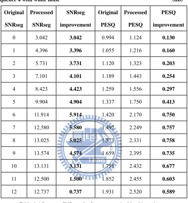
Sequence 4 with white noise (dB) Original SNRseg Processed SNRseg SNRseg improvement Original PESQ Processed PESQ PESQ improvement 0 3.042 3.042 0.994 1.124 0.130 1 4.396 3.396 1.055 1.216 0.160 2 5.731 3.731 1.120 1.323 0.203 3 7.101 4.101 1.189 1.443 0.254 4 8.423 4.423 1.259 1.556 0.297 5 9.904 4.904 1.337 1.750 0.413 6 11.914 5.914 1.420 2.170 0.750 7 12.580 5.580 1.492 2.249 0.757 8 13.025 5.025 1.573 2.331 0.758 9 13.574 4.574 1.659 2.395 0.735 10 13.131 3.131 1.755 2.432 0.677 11 12.500 1.500 1.852 2.455 0.603 12 12.737 0.737 1.931 2.520 0.589
Table 4-4 Segment SNR results for sequence 4 with white noise
46
Sequence 1 with babble noise (dB) Original SNRseg Processed SNRseg SNRseg improvement Original PESQ Processed PESQ PESQ improvement 0 2.919 2.919 1.283 1.498 0.214 1 4.294 3.294 1.326 1.546 0.220 2 5.331 3.331 1.369 1.629 0.260 3 6.267 3.267 1.422 1.711 0.289 4 7.019 3.019 1.475 1.778 0.303 5 7.507 2.507 1.531 1.851 0.320 6 8.177 2.177 1.573 1.907 0.333 7 9.208 2.208 1.639 1.982 0.343 8 10.708 2.708 1.712 2.052 0.340 9 11.262 2.262 1.775 2.103 0.327 10 11.891 1.891 1.851 2.184 0.333 11 12.752 1.752 1.940 2.234 0.293 12 13.013 1.013 2.006 2.301 0.294
Table 4-5 Segment SNR results for sequence 1 with babble noise
47
Sequence 2 with babble noise (dB) Original SNRseg Processed SNRseg SNRseg improvement Original PESQ Processed PESQ PESQ improvement 0 0.858 0.858 1.283 1.498 0.214 1 2.760 1.760 1.326 1.546 0.220 2 4.435 2.435 1.369 1.629 0.260 3 5.661 2.661 1.422 1.711 0.289 4 6.610 2.610 1.475 1.778 0.303 5 7.792 2.792 1.531 1.851 0.320 6 8.656 2.656 1.573 1.907 0.333 7 9.564 2.564 1.639 1.982 0.343 8 10.194 2.194 1.712 2.052 0.340 9 11.204 2.204 1.775 2.103 0.327 10 11.846 1.846 1.851 2.184 0.333 11 12.231 1.231 1.940 2.234 0.293 12 10.219 -1.781 2.006 2.301 0.294
Table 4-6 Segment SNR results for sequence 2 with babble noise
48
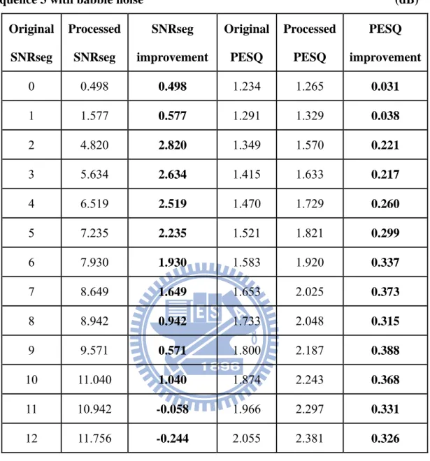
Sequence 3 with babble noise (dB) Original SNRseg Processed SNRseg SNRseg improvement Original PESQ Processed PESQ PESQ improvement 0 0.498 0.498 1.234 1.265 0.031 1 1.577 0.577 1.291 1.329 0.038 2 4.820 2.820 1.349 1.570 0.221 3 5.634 2.634 1.415 1.633 0.217 4 6.519 2.519 1.470 1.729 0.260 5 7.235 2.235 1.521 1.821 0.299 6 7.930 1.930 1.583 1.920 0.337 7 8.649 1.649 1.653 2.025 0.373 8 8.942 0.942 1.733 2.048 0.315 9 9.571 0.571 1.800 2.187 0.388 10 11.040 1.040 1.874 2.243 0.368 11 10.942 -0.058 1.966 2.297 0.331 12 11.756 -0.244 2.055 2.381 0.326
Table 4-7 Segment SNR results for sequence 3 with babble noise
49
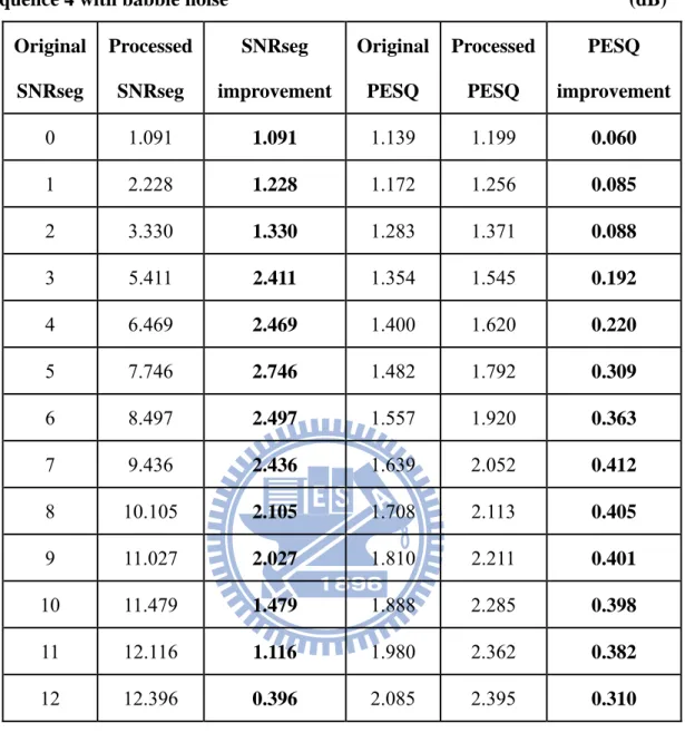
Sequence 4 with babble noise (dB) Original SNRseg Processed SNRseg SNRseg improvement Original PESQ Processed PESQ PESQ improvement 0 1.091 1.091 1.139 1.199 0.060 1 2.228 1.228 1.172 1.256 0.085 2 3.330 1.330 1.283 1.371 0.088 3 5.411 2.411 1.354 1.545 0.192 4 6.469 2.469 1.400 1.620 0.220 5 7.746 2.746 1.482 1.792 0.309 6 8.497 2.497 1.557 1.920 0.363 7 9.436 2.436 1.639 2.052 0.412 8 10.105 2.105 1.708 2.113 0.405 9 11.027 2.027 1.810 2.211 0.401 10 11.479 1.479 1.888 2.285 0.398 11 12.116 1.116 1.980 2.362 0.382 12 12.396 0.396 2.085 2.395 0.310
Table 4-8 Segment SNR results for sequence 4 with babble noise
50
Sequence 1 with factory noise (dB) Original SNRseg Processed SNRseg SNRseg improvement Original PESQ Processed PESQ PESQ improvement 0 4.912 4.912 1.074 1.406 0.332 1 6.001 5.001 1.112 1.490 0.377 2 6.749 4.749 1.150 1.523 0.372 3 7.359 4.359 1.207 1.610 0.403 4 7.851 3.851 1.259 1.646 0.387 5 8.248 3.248 1.295 1.710 0.415 6 10.268 4.268 1.357 1.854 0.496 7 11.187 4.187 1.421 1.956 0.535 8 11.934 3.934 1.489 2.022 0.533 9 12.561 3.561 1.537 2.102 0.565 10 13.133 3.133 1.610 2.166 0.556 11 13.096 2.096 1.703 2.253 0.550 12 13.685 1.685 1.787 2.304 0.517
Table 4-9 Segment SNR results for sequence 1 with factory noise