Open Access
Research article
Discovery of dominant and dormant genes from expression data
using a novel generalization of SNR for multi-class problems
Yu-Shuen Tsai
1, Chin-Teng Lin
2, George C Tseng
3, I-Fang Chung*
1and
Nikhil Ranjan Pal*
4Address: 1Institute of Biomedical Informatics, National Yang-Ming University, Taipei, Taiwan, 2Department of Electrical and Control Engineering,
Department of Computer Science, Brain Research Center, National Chiao-Tung University, Hsinchu, Taiwan, 3Department of Biostatistics,
Department of Human Genetics, Department of Computational Biology, University of Pittsburgh, USA and 4Electronics and Communication
Sciences Unit, Indian Statistical Institute, Calcutta, India
Email: Yu-Shuen Tsai - [email protected]; Chin-Teng Lin - [email protected]; George C Tseng - [email protected]; I-Fang Chung* - [email protected]; Nikhil Ranjan Pal* - [email protected]
* Corresponding authors
Abstract
Background: The Signal-to-Noise-Ratio (SNR) is often used for identification of biomarkers for two-class problems and no formal and useful generalization of SNR is available for multiclass problems. We propose innovative generalizations of SNR for multiclass cancer discrimination through introduction of two indices, Gene Dominant Index and Gene Dormant Index (GDIs). These two indices lead to the concepts of dominant and dormant genes with biological significance. We use these indices to develop methodologies for discovery of dominant and dormant biomarkers with interesting biological significance. The dominancy and dormancy of the identified biomarkers and their excellent discriminating power are also demonstrated pictorially using the scatterplot of individual gene and 2-D Sammon's projection of the selected set of genes. Using information from the literature we have shown that the GDI based method can identify dominant and dormant genes that play significant roles in cancer biology. These biomarkers are also used to design diagnostic prediction systems. Results and discussion: To evaluate the effectiveness of the GDIs, we have used four multiclass cancer data sets (Small Round Blue Cell Tumors, Leukemia, Central Nervous System Tumors, and Lung Cancer). For each data set we demonstrate that the new indices can find biologically meaningful genes that can act as biomarkers. We then use six machine learning tools, Nearest Neighbor Classifier (NNC), Nearest Mean Classifier (NMC), Support Vector Machine (SVM) classifier with linear kernel, and SVM classifier with Gaussian kernel, where both SVMs are used in conjunction with one-vs-all (OVA) and one-vs-one (OVO) strategies. We found GDIs to be very effective in identifying biomarkers with strong class specific signatures. With all six tools and for all data sets we could achieve better or comparable prediction accuracies usually with fewer marker genes than results reported in the literature using the same computational protocols. The dominant genes are usually easy to find while good dormant genes may not always be available as dormant genes require stronger constraints to be satisfied; but when they are available, they can be used for authentication of diagnosis.
Conclusion: Since GDI based schemes can find a small set of dominant/dormant biomarkers that is adequate to design diagnostic prediction systems, it opens up the possibility of using real-time qPCR assays or antibody based methods such as ELISA for an easy and low cost diagnosis of diseases. The dominant and dormant genes found by GDIs can be used in different ways to design more reliable diagnostic prediction systems.
Published: 9 October 2008
BMC Bioinformatics 2008, 9:425 doi:10.1186/1471-2105-9-425
Received: 16 January 2008 Accepted: 9 October 2008 This article is available from: http://www.biomedcentral.com/1471-2105/9/425
© 2008 Tsai et al; licensee BioMed Central Ltd.
This is an Open Access article distributed under the terms of the Creative Commons Attribution License (http://creativecommons.org/licenses/by/2.0), which permits unrestricted use, distribution, and reproduction in any medium, provided the original work is properly cited.
Background
Many studies have investigated the mechanism of carcino-genesis by analyzing the gene expression profiles from microarray data. Accurate diagnosis of different categories of cancers or identification of subgroups with homogene-ous molecular signature is important for proper treatment and prognosis. The application of gene expression data for these tasks is challenging because of its high dimensional nature and the noisy characteristics. Since the number of genes contained in each chip is far exceeding the number of available samples, the standard statistical methods for classification often do not work well. Therefore, identifi-cation of informative genes related to a set of diseases is an important subject in the field of biomedical informat-ics at least for two reasons: understanding the roles played by the genes in cancer biology and development of tools for efficient and accurate diagnostic prediction.
Many novel classification, clustering and prediction meth-odologies have been suggested to analyze gene expression data [1-4]. Here we need to deal with two problems: iden-tification of marker genes (this is a problem of dimension-ality reduction) and use of the marker genes for designing a diagnostic prediction system. For the second problem many machine learning tools, such as Neural Networks, Decision Trees, Nearest Neighbor Classifier, Naive Bayes classifier, Support Vector Machines have been used [5-8]. For the problem of gene selection also many methods have been proposed [2,4,7-10]. Gene selection methods can further be grouped into two categories: linear methods and non-linear methods.
The linear methods are very intuitive which exploit the linear relation between expression levels and the status of the disease. In other words, for a two-class problem, say Acute Lymphoblastic Leukemia (ALL) and Acute Myelog-enous Leukemia (AML), the high expression level may correspond to ALL while a low expression level may corre-spond to AML or vice versa. Two such indices are Signal-to-Noise ratio (SNR) [2] and correlation [7]. The SNR for
a gene g is defined as SNR(g) = (μ1(g) - μ2(g))/(σ1(g) +
σ2(g)), where μi(g) and σi(g) are the mean and standard
deviation of expression levels of a gene g for samples in class i (i = 1, 2), respectively. The authors in [7] adopted several formulae (Euclidean distance, Pearson correlation, SNR, etc.) for measuring the similarity between the
expression levels of a gene g and an ideal gene gideal in a
2-class problem, where an ideal gene pattern was defined by gideal = (gideal,1, 傼, gideal,G), gideal,j = 1, if the jth sample is from
class 1, otherwise gideal,j = 0; ∀ j = 1, 傼, G. The ideal values
can also be taken as 0 for class 1 and 1 for the class 2. Let
xg be the vector consisting of the expression values for a
gene g for all samples. Now the Pearson correlation or
cosine similarity between the two vectors gideal and xg can
be used to rank the genes. Although very intuitive, these
methods are neither easy to generalize to multiclass, nor such methods can take into account non-linear interac-tion between genes. The BW ratio [4] is a linear index that can be used for multiclass problems, but it is less intuitive and it is not easy to visualize its behavior.
Note that, there have been attempts to adapt two-class methods such as correlation for multiclass problems using the one-vs-all strategy [11]. In [11], first a set of genes is selected based on ANOVA. Then using this short-listed genes, a set of important genes is identified for each class by casting the problem into a two class problem. We call these method as ANOVA+Correlation method. For example, in a k-class problem, to get a set of important genes for class c, samples from class c are considered from class 1 and all samples from the remaining classes pooled together are treated as class 2. Then the correlation, as explained, in the previous paragraph is computed. Such a method will select strong marker genes, but may also select poor ones because the pooled class will have a much stronger and undesirable effect on the correlation than the class under consideration. Similarly, using the OVA strategy the SNR can also be used to select genes for a multiclass problem [12]. We shall call this method as OVA.SNR. In the OVA.SNR approach, for a k-class prob-lem, to select useful genes, say, for class 1, the data set is divided into two groups, data from class 1 and data from the the remaining 2 to k classes. Although such methods may find useful genes, in this case, the mean and standard deviation of the pooled group may not (usually will not) represent any useful information about the remaining classes. For example, in a 3-class problem, suppose for a gene, samples from each of the three classes are normally distributed (this is an assumption made while using ANOVA type tests). For simplicity, suppose we have n samples from each of the three classes and the mean and standard deviation computed from these samples for the
three classes are μi, σi; i = 1, 傼, 3, respectively. In the
OVA.SNR approach, the mean of the second group, does not represent the central tendency of the pooled group and hence it does not represent any useful information about the structure of the remaining two classes. Moreover, when samples from class 2 and class 3 are normally distributed with two different means, the pooled samples will not be normally distributed. Hence, OVA schemes, which use mean of the pooled class, for gene selection is not conceptually appealing, although such approaches may find useful discriminatory genes.
μ= μ2+μ3
On the other hand, the non-linear methods can take into account non-linear interaction between genes. There are several such methods, for example, online feature selec-tion using neural network [10], SVM-based recursive fea-ture elimination (SVM-RFE) [9], and the maximum margin criterion-based recursive feature elimination (MMC-RFE) [8]. In [10], the authors have considered the non-linear interaction between genes as well as that between genes and the tool used for gene selection. Although in [10] they have successfully discovered a small set of biomarkers for accurate prediction of cancer sub-groups, the behavior of non-linearly interacting genes is less interpretable than the linearly interacting genes for making simple decision rules. The SVM-RFE is a quite popular method of feature selection in an iterative man-ner. This method makes use of repeated training of a SVM classifier with a progressively reduced set of features. In every iteration, some of the less important features are removed. For a two-class problem, the SVM classifier finds
the weight vector, w ∈ Rp, p is the number of genes,
asso-ciated with the hyperplane that maximizes the margin of separation. The SVM-REF algorithm, trains SVM with all available genes first and finds the optimal weight vector w
∈ Rp. Then it computes a Ranking Criterion, RC, for each
gene. A possible choice of RC is (wi)2. Then either a single
gene (or a set of genes) with the smallest values of RC is removed and the process is then repeated with the reduced set of genes.
Here we aim to develop a gene selection method which is intuitive, can find useful marker genes and can be viewed as a true generalization of SNR. The GDI is akin to the SNR, which is widely used in two-class gene selection problems [2], but GDI can be applied to multicategory problems, and identifies dominant and dormant genes.
We define two indices named, Gene Dominant Index (GDI
-Dom) and Gene Dormant Index (GDIDor). The GDIDom leads
to the novel concept of Dominant Genes while the other index leads to the concept of Dormant Genes. A dominant gene is over-expressed in only one of the classes and under-expressed in the remaining classes, and thus has a very strong class specific signature. A dormant gene, on the other hand, is under-expressed in only one of the classes but over-expressed in the remaining classes, and thus also has a strong class specific signature. Clearly, dominant or dormant genes are good biomarkers, if they exist, and they are likely to play key roles in identifying sub-types/classes of disease. In order to reduce the effect of the finite sample size, we randomly select a part of the data to find a list of dominant and dormant genes. This process of random partition of data and computation of GDIs are repeated 100 times. The frequency with which different genes appear in the list of dominant and dor-mant genes is then computed. Since really good dominant and dormant genes are expected to appear more
fre-quently, we select a set of most frequently occurring dom-inant (dormant) genes. A set of strong domdom-inant and/or dormant genes, thus selected, can be used to design relia-ble diagnostic systems. Further details about the defini-tions and procedures can be found in the Materials and Methods section.
We want to emphasize that many genes may have discrim-inating power and hence can be considered marker genes but the dominant and dormant genes are special types of markers. Thus dominant and dormant genes are markers genes but all marker genes are not necessarily dominant/ dormant genes and GDI is designed to identify dominant/ dormant genes, if present. However, even if there are not many good dominant/dormant genes and we select a set of markers based on GDIs, such a set will do a good job of classification.
To compare the performance of our methods, we shall use six classifiers for diagnostic prediction: NMC, NNC, SVM with linear kernel, and SVM with Gaussian kernel. Each of the two SVMs is realized using both the OVA and OVO strategies and this makes the total number of classifiers to six. Our method is tested on four multi-class cancer data sets. We shall see later that our proposed methods can find a small set of discriminating biomarkers with excel-lent prediction accuracy.
Results and discussion
Four multicategory microarray gene expression data sets, namely, SRBCT (Small Round Blue Cell Tumors) [13], Leukemia [14], CNS (Central Nervous System Tumors) [15], and Lung Cancer [16] are used in this study for detailed analysis. We divide our discussion into three sub-sections, the biological relevance of some of the domi-nant/dormant genes, visual assessment of the dominant/ dormant marker genes, and comparison of classifier per-formance. The results obtained using SRBCT, Leukemia, and CNS are compared with those in [8]. The Lung Cancer data set (not used in [8]) is further used to show the effec-tiveness of our method. Details of the data sets can be found in Materials and Methods. We have followed the same experimental protocols as in [8] to make a proper comparison. Additionally, we have implemented the mul-ticlass version correlation based method (ANOVA+Corre-lation) and SNR (OVA.SNR) for comparison of performance.
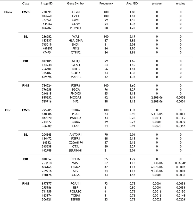
Biological relevance of some dominant/dormant genes Tables 1, 2, 3, 4, obtained by the Algorithm Gene Selection (see Materials and Methods), list the sets of dominant and dormant genes for the SRBCT, Leukemia, CNS, and Lung Cancer data sets, respectively. In Table 1 for the SRBCT data set, four of the most dominant genes, one for each
AF1Q, (d) FGFR4. The gene FCGRT (Fc fragment of IgG, receptor) has an EWS (Ewing sarcomas) specific signature because it is moderate to highly upregulated for the EWS group and is downregulated for the other three groups. This gene is known to play significant roles in other types of cancers too. For example, in [17] authors suggested a
set of 26 prognostic genes that can provide predictive information on the survival of patients suffering from lung cancer. They found that a higher expression level of FCGRT relates to a better survival outcome.
Table 1: Details of the selected genes by the frequency-based method for the SRBCT data set
Class Image ID Gene Symbol Frequency Ave. GDI p-value q-value
Dom EWS 770394 FCGRT 100 1.88 0 0 814260 FVT1 100 1.43 0 0 377461 CAV1 99 1.46 0 0 1435862 CD99 94 1.37 0 0 866702 PTPN13 88 1.28 0 0 BL 236282 WAS 100 2.19 0 0 183337 HLA-DMA 67 1.82 0 0 745019 EHD1 51 2.03 0 0 1469292 PIM2 24 1.90 0 0 47475 CYFIP2 24 1.85 0 0 NB 812105 AF1Q 99 1.65 0 0 134748 GCSH 64 1.45 0 0 756401 RHEB 56 1.41 0 0 325182 CDH2 33 1.38 0 0 629896 MAP1B 32 1.32 0 0 RMS 784224 FGFR4 100 1.60 0 0 796258 SGCA 96 1.27 0 0 244618 FNDC5 65 1.18 0 0 839552 NCOA1 42 1.14 2.60E-06 0.0002 769716 NF2 38 1.12 2.60E-06 0.0001 Dor EWS 295985 CDK6 100 1.37 0 0 448386 PBX3 73 0.96 5.11E-05 0.0011 842820 PABPC4 43 0.78 0.0011 0.0115 214572 CDK6 39 0.77 0.0003 0.0039 366009 LYAR 24 0.93 0.0078 0.0457 BL 204545 ANTXR1 70 2.04 0 0 154472 FGFR1 68 2.15 0 0 66552 C20orf194 57 2.12 0 0 345538 CTSL 50 2.27 0 0 142788 SERPINH1 21 2.04 0 0 NB 810057 CSDA 85 1.29 0 0
753418 VASP 62 1.16 1.73E-06 8.16E-05
686164 DGKZ 42 1.13 6.07E-06 0.0002 769716 NF2 34 1.12 9.53E-06 0.0003 128126 CD55 33 1.47 0.0003 0.0038 RMS 897177 PGAM1 73 0.75 0.0004 0.0053 295986 EBP 61 0.80 0.0004 0.0053 711959 POLR3C 41 0.72 0.0016 0.0150 163174 TCEA1 31 0.76 0.0016 0.0148 306921 EEF1E1 23 0.72 0.0028 0.0224
The WAS gene belongs to the set of Human Cancer Genes [18]. It has a very strong BL (Burkitt lymphomas) class specific signature, and it is also found important by others in the context of the SRBCT data set [19]. The relationship of WAS to Burkitt Lymphomas is also reported in [20]. The deficiency of WAS gene causes the Wiskott-Aldrich syndrome, which is an X-linked hereditary disease associ-ating primary immunodeficiency, thrombocytopenia, an increased risk of autoimmune diseases and malignancies, particularly non-Hodgkin's lymphoma (NHL) [21-24]. In patients with Wiskott-Aldrich syndrome, a higher rate of malignancy has been observed, particularly in Epstein-Barr Virus-related brain tumor, leukemia and lymphoma http://www.stjude.org. Amongst the different kinds of tumors, the most frequently associated one with Wiskott-Aldrich syndrome is the NHL tumor (it is about 76%).
The other kinds of tumors associated with WAS include, Hodgkin's disease, glioma, and testicular carcinoma [21,24]. Although NHL is the most common type of malignancy found in WAS and BL represents 40% to 50% of all NHL cases in childhood, BL has hardly been reported in WAS. But a case of BL with WAS is reported in [20]. In [24], authors reported Malignant B Cell Non-Hodgkin's Lymphoma of the Larynx with Wiskott-Aldrich syndrome. All these clearly establishes the important role of WAS not only in BL, but in other types of malignancies too.
The ALL1-fused gene from chromosome 1q (AF1Q) is one of the dominant genes found by our method for the neu-roblastoma (NB) group. Many authors have reported this gene to play important roles in cancer [25,26]. As revealed Table 2: Details of the selected genes by the frequency-based method for the Leukemia data set
Class Probe ID Gene Symbol Frequency Ave. GDI p-value q-value
Dom ALL 1389_at MME 96 1.98 0 0
32847_at MYLK 62 2.02 0 0 32872_at ESTs 58 1.73 0 0 35164_at WFS1 52 2.05 0 0 37280_at SMAD1 25 1.87 0 0 MLL 34306_at MBNL1 99 1.43 0 0 40763_at MEIS1 92 1.41 0 0 36777_at KLRK1 83 1.42 0 0 1065_at FLT3 56 1.20 0 0 34583_at FLT3 30 1.30 0 0
AML 39566_at CHRFAM7A 46 1.89 0 0
41752_at GHITM 39 1.51 0 0
38710_at OTUB1 31 1.54 0 0
37187_at CXCL2 22 1.53 0 0
36162_at BSG 21 1.47 0 0
Dor ALL 33412_at LGALS1 94 1.66 0 0
37403_at ANXA1 90 1.74 0 0
37809_at HOXA9 62 1.59 0 0
41448_at HOXA10 54 1.64 0 0
31575_f_at ESTs 33 1.65 0 0
MLL 1674_at YES1 69 1.03 0 0
1325_at SMAD1 43 0.97 9.54E-07 2.80E-05
539_at RYK 39 1.05 0 0
1971_g_at FHIT 33 0.90 9.54E-07 3.02E-05
37527_at ELK3 28 0.98 9.54E-07 2.81E-05
AML 41747_s_at MEF2A 50 1.89 0 0
41503_at ZHX2 49 1.88 0 0
37988_at CD79B 37 1.98 0 0
37710_at MEF2C 34 2.04 0 0
40966_at STK39 32 2.12 0 0
Table 3: Details of the selected genes by the frequency-based method for the CNS data set
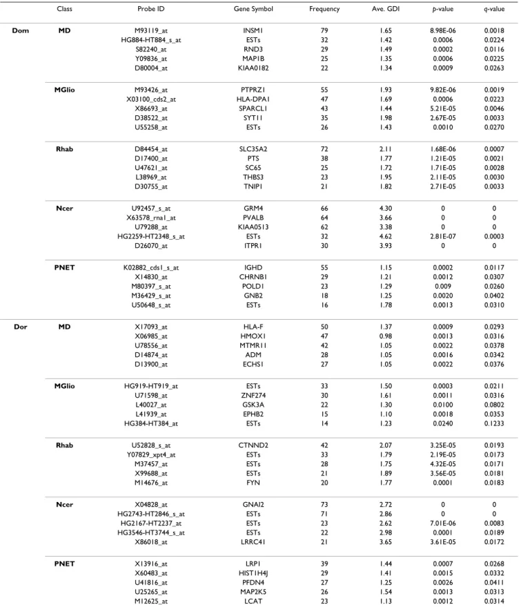
Class Probe ID Gene Symbol Frequency Ave. GDI p-value q-value
Dom MD M93119_at INSM1 79 1.65 8.98E-06 0.0018
HG884-HT884_s_at ESTs 32 1.42 0.0006 0.0224
S82240_at RND3 29 1.49 0.0002 0.0116
Y09836_at MAP1B 25 1.35 0.0006 0.0225
D80004_at KIAA0182 22 1.34 0.0009 0.0263
MGlio M93426_at PTPRZ1 55 1.93 9.82E-06 0.0019
X03100_cds2_at HLA-DPA1 47 1.69 0.0006 0.0223
X86693_at SPARCL1 43 1.44 5.21E-05 0.0046
D38522_at SYT11 35 1.98 2.67E-05 0.0033
U55258_at ESTs 26 1.43 0.0010 0.0270
Rhab D84454_at SLC35A2 72 2.11 1.68E-06 0.0007
D17400_at PTS 38 1.77 1.21E-05 0.0021
U47621_at SC65 25 1.72 1.71E-05 0.0028
L38969_at THBS3 23 1.95 2.11E-05 0.0030
D30755_at TNIP1 21 1.82 2.71E-05 0.0033
Ncer U92457_s_at GRM4 66 4.30 0 0
X63578_rna1_at PVALB 64 3.66 0 0
U79288_at KIAA0513 62 3.38 0 0
HG2259-HT2348_s_at ESTs 32 4.62 2.81E-07 0.0003
D26070_at ITPR1 30 3.93 0 0
PNET K02882_cds1_s_at IGHD 55 1.15 0.0002 0.0117
X14830_at CHRNB1 29 1.21 0.0012 0.0307
M80397_s_at POLD1 23 1.29 0.009 0.0260
M36429_s_at GNB2 18 1.25 0.0020 0.0402
U50648_s_at ESTs 16 1.78 0.0013 0.0310
Dor MD X17093_at HLA-F 50 1.37 0.0009 0.0293
X06985_at HMOX1 47 0.98 0.0013 0.0316
U78556_at MTMR11 42 1.05 0.0022 0.0378
D14874_at ADM 28 1.05 0.0016 0.0342
D13900_at ECHS1 27 1.05 0.0022 0.0376
MGlio HG919-HT919_at ESTs 33 1.50 0.0003 0.0211
U71598_at ZNF274 30 1.61 0.0011 0.0316
L40027_at GSK3A 22 1.30 0.0100 0.0802
L41939_at EPHB2 15 1.10 0.0018 0.0353
HG384-HT384_at ESTs 14 1.23 0.0240 0.1233
Rhab U52828_s_at CTNND2 42 2.07 3.25E-05 0.0193
Y07829_xpt4_at ESTs 33 1.79 2.19E-05 0.0173
M37457_at ESTs 28 1.75 4.32E-05 0.0171
X99688_at ESTs 21 1.89 3.56E-05 0.0181
M14676_at FYN 20 1.77 0.0001 0.0183
Ncer X04828_at GNAI2 73 2.72 0 0
HG2743-HT2846_s_at ESTs 71 2.86 0 0
HG2167-HT2237_at ESTs 23 2.62 7.01E-06 0.0083
HG3546-HT3744_s_at ESTs 22 2.98 0.0001 0.0189 X86018_at LRRC41 21 3.65 3.61E-05 0.0172 PNET X13916_at LRP1 39 1.44 0.0007 0.0268 X60483_at HIST1H4J 29 1.41 0.0015 0.0332 U41816_at PFDN4 27 1.25 0.0026 0.0411 U25265_at MAP2K5 26 1.54 0.0013 0.0313 M12625_at LCAT 23 1.13 0.0012 0.0314
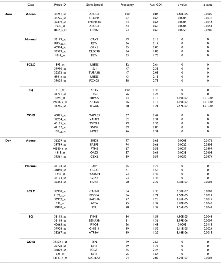
Table 4: Details of the selected genes by the frequency-based method for the Lung Cancer data set
Class Probe ID Gene Symbol Frequency Ave. GDI p-value q-value
Dom Adeno 38261_at ABCC3 100 0.84 2.68E-05 0.0005
35276_at CLDN4 77 0.66 0.0004 0.0038
39339_at TMEM63A 63 0.64 0.0005 0.0044
1930_at ABCC3 43 0.68 0.0006 0.0051
1802_s_at ERBB2 23 0.68 0.0053 0.0280
Normal 36119_at CAV1 99 2.13 0 0
1815_g_at ESTs 36 2.14 0 0 40994_at GRK5 35 2.00 0 0 36569_at CLEC3B 34 1.83 0 0 1814_at ESTs 33 1.75 0 0 SCLC 893_at UBE2S 52 2.64 0 0 39990_at ISL1 47 2.38 0 0 32272_at TUBA1B 47 2.05 0 0 894_g_at UBE2S 43 2.18 0 0 39605_at FOXG1 38 2.78 0 0 SQ 613_at KRT5 100 1.48 0 0 31791_at TP63 96 1.26 0 0
1898_at TRIM29 74 1.18 3.19E-07 1.61E-05
39016_r_at KRT6A 56 1.18 3.19E-07 1.51E-05
41266_at ITGA6 38 1.21 9.57E-07 4.21E-05
COID 40825_at MAPRE3 67 2.47 0 0
32254_at VAMP2 52 2.31 0 0
40165_at TSPYL2 49 2.36 0 0
41107_at SNPH 39 2.80 0 0
198_g_at NME3 26 2.31 0 0
Dor Adeno 36209_at BRD2 97 0.68 0.0008 0.0176
39799_at FABP5 74 0.66 0.0022 0.0305 40580_r_at PTMS 67 0.58 0.0037 0.0399 1315_at OAZ1 57 0.61 0.0038 0.0408 39561_at CBX6 39 0.59 0.0050 0.0474 Normal 36133_at DSP 55 1.73 0 0 31850_at GCLC 41 1.58 0 0 1248_at POLR2H 23 1.48 0 0 35194_at GPX2 23 1.46 0 0
39353_at HSPE1 20 2.29 6.38E-07 0.0003
SCLC 33908_at CAPN1 54 1.30 6.38E-07 0.0003
1109_s_at PDGFA 36 1.71 1.50E-05 0.0022
36952_at HADHA 27 1.28 1.26E-05 0.0019
338_at ATF6 25 1.32 5.70E-05 0.0046
36890_at PPL 20 1.32 4.55E-05 0.0042
SQ 38113_at SYNE1 34 1.51 4.90E-05 0.0043
33118_at SEMA3B 31 1.36 3.99E-06 0.0009
40665_at FMO3 26 1.48 0.0003 0.0115
37908_at GNG11 19 1.52 2.11E-05 0.0024
33267_at ATP8A1 19 1.22 8.14E-06 0.0015
COID 33322_i_at SFN 79 2.67 0 0
39728_at ESTs 39 1.75 0 0
36879_at ECGF1 35 2.24 0 0
925_at ESTs 25 1.64 0 0
33143_s_at SLC16A3 24 2.07 4.79E-07 0.0003
by Fig. 1(c), AF1Q is moderate to highly express for the neuroblastoma cases, while it exhibits low expression val-ues for the other three groups of the SRBCT.
As discussed in [10,27], FGFR4 carries out the signal trans-duction to the intracellular environment in cellular
prolif-eration, differentiation and migration. Overexpression of FGFR4 is found in various cancers, such as of pituitary, prostate, thyroid [28-30], but in normal tissues, FGFR4 expression is hardly noticeable. In our study with the SRBCT, we noticed a very strong RMS (rhabdomyosarco-mas) specific signature, very high expression levels of
Scatterplots of the most dominant gene in each subgroup of the SRBCT data set: (a) FCGRT (Image: 770394) for EWS, (b) WAS (Image: 236282) for BL, (c) AF1Q (Image: 812105) for NB, (d) FGFR4 (Image: 784224) for RMS
Figure 1
Scatterplots of the most dominant gene in each subgroup of the SRBCT data set: (a) FCGRT (Image: 770394) for EWS, (b) WAS (Image: 236282) for BL, (c) AF1Q (Image: 812105) for NB, (d) FGFR4 (Image: 784224) for RMS. 0 10 20 30 40 50 60 0. 0 0 .2 0. 4 0 .6 0. 8 1 .0 Samples G ene Expr ess io n V a lues EWS BL NB RMS 0 10 20 30 40 50 60 0. 0 0 .2 0. 4 0 .6 0. 8 1 .0 Samples G ene Expr ess io n V a lues EWS BL NB RMS 0 10 20 30 40 50 60 0. 0 0 .2 0. 4 0 .6 0. 8 1 .0 Samples G ene Expr ess io n V a lues EWS BL NB RMS 0 10 20 30 40 50 60 0. 0 0 .2 0. 4 0 .6 0. 8 1 .0 Samples G ene Expr ess io n V a lues EWS BL NB RMS
(a)
(b)
(c)
(d)
FGFR4 for the RMS group, but for the other groups it is practically unexpressed. However, in lung adenoarci-noma, FGFR4 is found to be downregulated [31]. The second and third most dominant genes for the EWS class are Follicular lymphoma variant translocation 1 (FVT1) and CAV1 (caveolin 1, caveolae protein, 22 kD). According to [32] FVT1 is found to be weakly expressed in normal hematopoietic tissues, but is shown to exhibit a very high rate of transcription in some T-cell malignancies and in phytohemagglutinin-stimulated lymphocytes. Becuase of the proximity of FVT1 to BCL2, authors in [32] also have indicated that both genes may involve in the tumoral process. For the present data set, it exhibits a very strong EWS specific signature. Its expression is practically absent for RMS, NB and NHL groups, but it is highly expressed for the EWS group. The gene CAV1 is also a bio-logically informative gene. In our study we found CAV1 to be upregulated for the EWS group. According to [33], CAV1 is down-regulated in oncogene-transformed and tumor-derived cells and it is an essential structural constit-uent of caveolae that plays important roles in mitogenic signaling and oncogenesis. Many studies have reported CAV1 as a candidate tumor suppressor gene [34-36]. It has been established that CAV1 has tumor suppressor activity in human cancers, including breast cancer [33,37], ovar-ian cancer [38], and lung cancer [39]. But in [40], they showed that CAV1 is over-expressed in human gastric can-cer cell line GTL-16. Also, for diffuse large B-cell lym-phoma [41] and prostate cancer [42], CAV1 is identified to serve as a diagnostic and prognostic marker. For the Lung Cancer data set in this study we have found CAV1 as a good dominant gene for the normal tissue group and this is in conformity with the fact that CAV1 also plays the role of a tumor suppressor. This is also consistent with down-regulation of CAV1 in human lung carcinoma [39]. Thus, CAV1 plays an important role in cancer biology. According to Table 2, we shall now discuss the importance of some dominant and dormant genes for the Leukemia data set. The MME (membrane metallo-endopeptidase), also known as CD10, is the most important dominant
gene for the ALL group as found by GDIDom. MME is found
to play different roles in different types of cancers. In [43], authors suggested that the functions of MME vary with tis-sue types and disease states. For example, in hepatocellu-lar and thyroid carcinoma MME exhibits higher expression levels [44,45], while in poorly differentiated tumors in the colon and stomach MME shows low expres-sion levels [46]. According to [47], MME is downregulated in the ALL samples with MLL (Mixed-Lineage Leukemia) rearrangements compared to ALL without MLL rearrange-ments. In our study we have found MME to be highly expressed in ALL while for the MLL and AML groups it is moderately expressed.
The top two dominant genes for the MLL group found by GDI are MBNL1 and MEIS1. In our study, we have found that expression levels of both MBNL1 and MEIS1 are higher for the MLL group than the other two groups. In [48], authors have found upregulation of these two genes in the ALL and AML groups with MLL chimeric fusion genes. It is interesting to know that by just using three genes MME and MBNL1 and MEIS1, one can do a good job of discrimination between the three types of leukemia (results not shown); of course, three dominant genes, one from each class can do an excellent job of classification too.
The most dormant gene for the ALL class as detected by
GDIDor is LGALS1. In [49] it is claimed that a higher
expression of LGALS1 is a negative prognostic predictor of recurrence in laryngeal squamous cell carcinomas. The next important dormant gene for the same class is ANXA1. This gene has been extensively studied and is found to play interesting roles in human cancers. Following [50,51] we summarize various cases where ANXA1 is up-regulated and down-up-regulated. Higher expression level of ANXA1 is observed in hepatocellular carcinoma [52], mammary adenocarcinoma [53], glioblastoma [54], and pancreatic cancer [55]. On the other hand, many investi-gations have reported down-regulation of ANXA1 in dif-ferent types of cancers such as in the head and neck [56,57], esophageal [56], prostate [56], breast [50], and larynx [51]. In our study with the leukemia data set, ANXA1 is identified as a good dormant gene for the ALL group. Note that, an absence of ANAX1 expression is observed in B-cell non-Hodgkin's lymphomas too [58]. In our investigation with the CNS data set, as shown in Table 3, the transcriptional repressor, insulinoma-associ-ated 1 (INSM1) is found to be one of the dominant genes for the MD (medulloblastomas) group. Different investi-gations have found this gene to play roles in tumors of neuroendocrine origin. In [59], they reported INSM1 as one of the important genes in discriminating pancreatic adenocarcinomas and islet cell tumors from normal pan-creatic tissues. The gene INSM1 is also found to be over-expressed in small-cell lung cancer (SCLC), SCLC cell lines as well as in medullary thyroid carcinoma, insuli-noma, and pituitary tumors [16,60,61].
As shown in Table 4, the most important dominant gene for the Adenocarcinoma group of the lung cancer data is ABCC3. The protein encoded by this gene belongs to the superfamily of ATP-binding cassette (ABC) transporters and is known to be involved in multi-drug resistance. The roles played by ABCC3 in different cancers are also reported in the literature [62-64]. For example, O'Brien et al. [62] have claimed that amplification and concomitant overexpression of the gene ABCC3 is responsible to confer
resistance to paclitaxel and monomethyl-auristatin-E. Authors also demonstrated that this amplification is present in primary breast tumors. Benderra et al. [64] have suggested that ABCC3 may be involved in chemoresist-ance in AML. The GDI based method has identified
Kera-tin 5 (KRT5) as the most dominant gene for the squamous cell lung carcinoma (SQ) group. An inspection of Fig. 7 reveals that for most of the SQ samples KRT5 is highly expressed while its expression level for the other four groups in the Lung Cancer data set is practically absent.
Scatterplots of the most dormant gene in each subgroup of the SRBCT data set: (a) CDK6 (Image: 295985) for EWS, (b) ANTXR1 (Image: 204545) for BL, (c) CSDA (Image: 810057) for NB, (d) PGAM1 (Image: 897177) for RMS
Figure 2
Scatterplots of the most dormant gene in each subgroup of the SRBCT data set: (a) CDK6 (Image: 295985) for EWS, (b) ANTXR1 (Image: 204545) for BL, (c) CSDA (Image: 810057) for NB, (d) PGAM1 (Image: 897177) for RMS.
(a)
(b)
(c)
(d)
0 10 20 30 40 50 60 0. 0 0 .2 0. 4 0 .6 0. 8 1 .0 Samples G ene Expr ess io n V a lues EWS BL NB RMS 0 10 20 30 40 50 60 0. 0 0 .2 0. 4 0 .6 0. 8 1 .0 Samples G ene Expr ess io n V a lues EWS BL NB RMS 0 10 20 30 40 50 60 0. 0 0 .2 0. 4 0 .6 0. 8 1 .0 Samples G ene Expr ess io n V a lues EWS BL NB RMS 0 10 20 30 40 50 60 0. 0 0 .2 0. 4 0 .6 0. 8 1 .0 Samples G ene Expr ess io n V a lues EWS BL NB RMSThis strong SQ specific signature of KRT5 is also reported in [65,66].
Visual assessment of the dominant/dormant marker genes In the next section we shall demonstrate the utility of the identified genes through performance comparison with different classifiers. But classifier performance is an
indi-rect indicator. It does not reveal how dominant (dor-mant) a gene is with respect to a class. So we try to make visual assessments of the quality of the dominant (dor-mant) genes. For this we adopt two approaches. First, we use scatterplots to view the distribution of the expression values of a dominant (dormant) gene in all samples (not including samples of the independent data set). This helps
Scatterplots of the most dominant gene in each subgroup of the Leukemia data set: (a) MME (1389_at) for ALL, (b) MBNL1 (34306_at) for MLL, (c) CHRFAM7A (39566_at) for AML
Figure 3
Scatterplots of the most dominant gene in each subgroup of the Leukemia data set: (a) MME (1389_at) for ALL, (b) MBNL1 (34306_at) for MLL, (c) CHRFAM7A (39566_at) for AML.
(a)
(b)
(c)
0 10 20 30 40 50 0. 0 0 .2 0. 4 0 .6 0. 8 1 .0 Samples G ene Expr ess io n V a lues ALL MLL AML 0 10 20 30 40 50 0. 0 0 .2 0. 4 0 .6 0. 8 1 .0 Samples G ene Expr ess io n V a lues ALL MLL AML 0 10 20 30 40 50 0. 0 0 .2 0. 4 0 .6 0. 8 1 .0 Samples G ene Expr ess io n V a lues ALL MLL AMLus to assess the discriminating power of (each) individual gene. Second, we try to visualize the overall discriminat-ing power of a set of dominant (dormant) genes selected based on GDIs. This is done by looking at a two-dimen-sional plot generated using Sammon's Non-linear Projec-tion [67] that preserves the inter-point distances in the
high dimensional space. Note that, Sammon's method does not use class information. The plots are labeled using the class information just for better visualization. For the Leukemia and SRBCT data sets, in the Sammon's plot we include both the training and independent data sets (for the training data different classes are represented by
differ-Scatterplots of the most dormant gene in each subgroup of the Leukemia data set: (a) LGALS1 (33412_at) for ALL, (b) YES1 (1674_at) for MLL, (c) MEF2A (41747_s_at) for AML
Figure 4
Scatterplots of the most dormant gene in each subgroup of the Leukemia data set: (a) LGALS1 (33412_at) for ALL, (b) YES1 (1674_at) for MLL, (c) MEF2A (41747_s_at) for AML.
(a)
(b)
(c)
0 10 20 30 40 50 0. 0 0 .2 0. 4 0 .6 0. 8 1 .0 Samples G ene Expr ess io n V a lues ALL MLL AML 0 10 20 30 40 50 0. 0 0 .2 0. 4 0 .6 0. 8 1 .0 Samples G ene Expr ess io n V a lues ALL MLL AML 0 10 20 30 40 50 0. 0 0 .2 0. 4 0 .6 0. 8 1 .0 Samples G ene Expr ess io n V a lues ALL MLL AMLent shapes with different colors; for the independent test data, the same shapes are used but filled in with colors). In Figs. 1, 2, 3, 4, 5, 6, 7, 8, the y-axis expresses the observed gene expression values (normalized in [0,1]), the x-axis indicates the samples in a data set. The samples in different groups (classes) are represented by different symbols and colors. The four panels in Fig. 1 display the four most dominant (one for each class) genes for the SRBCT data set. As expected, the dominant gene for a class appears with high expression values in the samples from that class, but with low expression values in the samples of the other classes/subgroups. As an example, for the SRBCT data set the most dominant gene, FCGRT (Image: 770394), for the Ewing Sarcoma is highly expressed for the EWS group while, it is practically unexpressed for the other three SRBCT classes (Fig. 1(a)). Similarly, Fig. 1(b)
shows that for the Burkitt Lymphomas (BL) the most dominant gene, WAS (Image: 236282), is over-expressed for the BL samples but under-expressed for the other classes.
Figure 2 depicts that for the SRBCT the dormant genes for all four classes are not very good and that explains the poor performance of the classifiers discussed later. In Fig. 2 we find that the most dormant gene, CDK6 (Image: 295985), for the EWS is completely unexpressed for the EWS samples while it is moderately expressed for the remaining three classes. Of the remaining three classes, the average expression level for the BL group is the closest to that of EWS group. Although, from pattern recognition point of view, this gene can distinguish EWS from the other three classes, since the difference between the aver-age expression levels for EWS and BL groups is not high,
Scatterplots of the most dominant gene in each subgroup of the CNS data set: (a) INSM1 (M93119_at) for MD, (b) PTPRZ1 (M93426_at) for MGlio, (c) SLC35A2 (D84454_at) for Rhab, (d) GRM4 (U92457_s_at) for Ncer, (e) IGHD (K02882 cds1_s_at) for PNET
Figure 5
Scatterplots of the most dominant gene in each subgroup of the CNS data set: (a) INSM1 (M93119_at) for MD, (b) PTPRZ1 (M93426_at) for MGlio, (c) SLC35A2 (D84454_at) for Rhab, (d) GRM4 (U92457_s_at) for Ncer, (e) IGHD (K02882 cds1_s_at) for PNET.
(a)
(b)
(d)
(e)
0 10 20 30 40 0. 0 0 .2 0. 4 0 .6 0 .8 1 .0 Samples G e ne E x pr es si o n V a lu e s MD MGlio Rhab Ncer PNET 0 10 20 30 40 0. 0 0 .2 0. 4 0 .6 0 .8 1 .0 Samples G e ne E x pr es si o n V a lu e s MD MGlio Rhab Ncer PNET 0 10 20 30 40 0 .0 0 .2 0 .4 0 .6 0 .8 1 .0 Samples G e ne E x pr es si o n V a lu e s MD MGlio Rhab Ncer PNET 0 10 20 30 40 0 .0 0 .2 0 .4 0 .6 0 .8 1 .0 Samples G e ne E x pr es si o n V a lu e s MD MGlio Rhab Ncer PNET 0 10 20 30 40 0 .0 0 .2 0 .4 0 .6 0 .8 1 .0 Samples G e ne E x pr es si o n V a lu e s MD MGlio Rhab Ncer PNET(c)
this gene may not be considered a very good dormant gene. In some cases, the identified dormant genes may not even be good from pattern recognition point of view also. As an example, consider Fig. 2(d) depicting the expression values of the most dormant gene for the RMS group. Clearly, the distribution of expression levels reveals that this gene cannot distinguish the RMS group from the EWS and NB groups. This is an indicator that for the RMS group we do not have any good dormant gene. This can be
checked from the average values of GDIDor in Table 1. For
the EWS and BL groups the average GDIDor values for the
most dormant genes are 1.37 and 2.04 respectively, while for the RMS group it is only 0.75.
The scatterplots of three most dominant genes for the Leukemia data set, one for each class, are displayed in Fig. 3. Fig. 3(a) depicts that the gene MME has a very strong
ALL specific signature and Fig. 3(c) representing CHRFAM7A has a strong signature for the AML group; while the gene MBNL1 (Fig. 3(b)) although has an MLL specific signature, it is not as strong as that of the other two genes. Fig. 4 depicts the scatterplots of the most dor-mant genes for Leukemia data set. Here we find that for majority of the samples in the ALL group, the most dor-mant gene, LGALS1, takes low expression values com-pared to the samples from the other two groups. In this case the separation between the average expression values between the ALL and AML groups is quite high making it a good dormant gene. This is also revealed by the GDI val-ues of 1.66. Similarly, for the AML class, the most dor-mant gene, MEF2A, is downregulated for the AML group, while it is upregulated for the remaining groups (the aver-age GDI value is 1.89). Thus, this gene can also be consid-ered a good dormant gene.
Scatterplots of the most dormant gene in each subgroup of the CNS data set: (a) HLA-F (X17093_at) for MD, (b) ESTs (HG919-HT919_at) for MGlio, (c) CTNND2 (U52828_s_at) for Rhab, (d) GNAI2 (X04828_at) for Ncer, (e) LRP1 (X13916_at) for PNET
Figure 6
Scatterplots of the most dormant gene in each subgroup of the CNS data set: (a) HLA-F (X17093_at) for MD, (b) ESTs (HG919-HT919_at) for MGlio, (c) CTNND2 (U52828_s_at) for Rhab, (d) GNAI2 (X04828_at) for Ncer, (e) LRP1 (X13916_at) for PNET.
(a)
(b)
(d)
(e)
0 10 20 30 40 0 .0 0 .2 0 .4 0 .6 0 .8 1 .0 Samples G ene E x p res s ion V alues MD MGlio Rhab Ncer PNET 0 10 20 30 40 0 .00 .2 0 .40 .6 0 .8 1 .0 Samples G e n e E x pr es sio n V a lu es MD MGlio Rhab Ncer PNET 0 10 20 30 40 0 .00 .2 0 .40 .6 0 .8 1 .0 Samples G e n e E x pr es sio n V a lu es MD MGlio Rhab Ncer PNET 0 10 20 30 40 0 .0 0 .2 0 .4 0 .6 0 .8 1 .0 Samples G ene E x p res s ion V alues MD MGlio Rhab Ncer PNET 0 10 20 30 40 0 .0 0 .2 0 .4 0 .6 0 .8 1 .0 Samples G ene E x p res s ion V alues MD MGlio Rhab Ncer PNET(c)
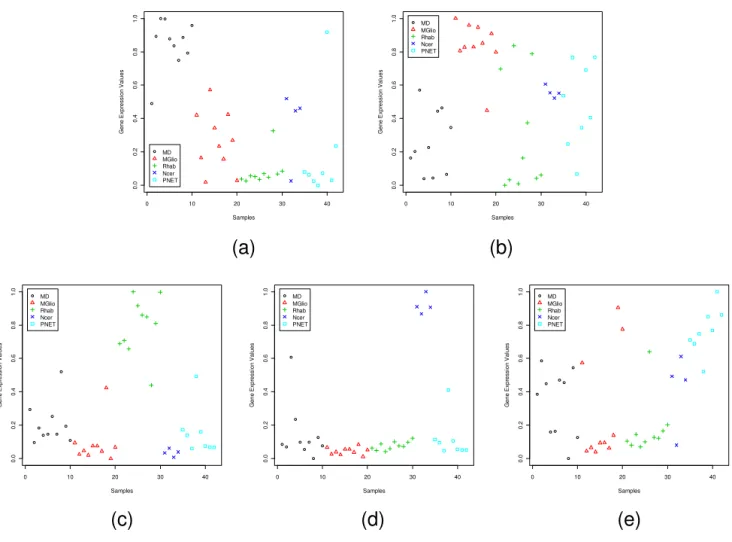
Figures 5 and 6 display the scatterplots of the dominant and dormant genes, respectively, for the CNS data set while Figs. 7 and 8 depict the same for the Lung Cancer data set. The Lung Cancer data set have five subgroups. Except for the adenocarcinoma group, each of the remain-ing subgroups has a dominant gene with very strong group specific signature. The adenocarcinoma group has the largest number of samples. Although, on average the dominant gene for this group has a higher expression level, there are several samples with low expression values too.
Now we shall analyze sets of genes selected by our method using Sammon's Projection (Figs. 9, 10, 11, 12). We use the function "sammon" in MASS library in R http:// www.r-project.org in conjunction with random initial configuration. For each class we select all top five selected
dominant genes. For example, in case of SRBCT we have used 20 dominant genes, five from each of the four classes. For the scatterplots we have used the normalized expression values for an easy visual assessment, but here since we want to preserve inter-point distances, we use the data obtained after preprocessing. For the SRBCT data set, the Sammon's plot is shown in Fig. 9(a). In Fig. 9(a), for the training data different classes are represented by differ-ent shapes with differdiffer-ent colors. For the independdiffer-ent test data, we use the same shapes but filled in with colors. For example, if the training data from a class is represented by red empty square, then the test data from the same class will be represented by filled in red square. Figure 9(a) reveals that samples from different classes form nice clus-ters both for the training and independent data sets, although the gene selection is done exclusively based on the training set. Figure 9(b) depicts the Sammon's plot
Scatterplots of the most dominant gene in each subgroup of the Lung Cancer data set: (a) ABCC3 (38261_at) for Adeno, (b) CAV1 (36119_at) for Normal, (c) UBE2S (893_at) for SCLC, (d) KRT5 (613_at) for SQ, (e) MAPRE3 (40825_at) for COID
Figure 7
Scatterplots of the most dominant gene in each subgroup of the Lung Cancer data set: (a) ABCC3 (38261_at) for Adeno, (b) CAV1 (36119_at) for Normal, (c) UBE2S (893_at) for SCLC, (d) KRT5 (613_at) for SQ, (e) MAPRE3 (40825_at) for COID.
(a)
(b)
(c)
(d)
(e)
0 50 100 150 200 0 .00 .2 0 .40 .6 0 .81 .0 Samples G e ne E x pr ess ion V alues Adeno Normal SCLC SQ COID 0 50 100 150 200 0. 0 0 .2 0. 4 0 .6 0. 8 1 .0 Samples G ene E x pr es sion V alues Adeno Normal SCLC SQ COID 0 50 100 150 200 0. 0 0 .2 0. 4 0 .6 0. 8 1 .0 Samples G ene E x pr es sion V alues Adeno Normal SCLC SQ COID 0 50 100 150 200 0 .00 .2 0 .40 .6 0 .81 .0 Samples G e ne E x pr ess ion V alues Adeno Normal SCLC SQ COID 0 50 100 150 200 0 .00 .2 0 .40 .6 0 .81 .0 Samples G e ne E x pr ess ion V alues Adeno Normal SCLC SQ COIDusing the dormant genes. Comparing the Sammon's plot with the dominant genes, we find that although the dor-mant genes approximately reveal the class structures, these are not as clear as in the case of the dominant genes. In fact, there are some mixing up of the groups. This explains the poor test performance obtained with the dor-mant genes (details in the next section).
For the Leukemia data set, Figs. 10(a) and 10(b) display the Sammon's plots using dominant and dormant genes considering the training and independent data sets together. Unlike, SRBCT here for both dominant and dor-mant genes the three classes are almost well separated. This is in conformity with comparable and good perform-ance of all six classifiers using the dominant and dormant genes (discussed in the next section). These results imply that the dominant or dormant genes selected from each
subgroup of the microarray data set contribute good dis-crimination power between classes.
For the CNS and the Lung Cancer data sets there is no independent test data set. Figs. 11 and 12 show the Sam-mon's plots for these two data sets. In the case of CNS, with dominant genes, the Sammon's plot exhibits very nice class structure for all classes (only one point of PNET, primitive neuro-ectodermal tumors, class is mixed up). But for the dormant genes, all but PNET class form nice clusters in the Sammon's plot. For the Lung Cancer data although with the dominant genes the class structures emerge in the Sammon's plot, with the dormant genes the COID (pulmonary carcinoids) group stands out sepa-rately but other classes are overlapped. This should not be used to infer that the performance of classifiers using the dormant genes would be poor – this is not indeed the
Scatterplots of the most dormant gene in each subgroup of the Lung Cancer data set: (a) BRD2 (36209_at) for Adeno, (b) DSP (36133_at) for Normal, (c) CAPN1 (33908_at) for SCLC, (d) SYNE1 (38113_at) for SQ, (e) SFN (33322_i_at) for COID
Figure 8
Scatterplots of the most dormant gene in each subgroup of the Lung Cancer data set: (a) BRD2 (36209_at) for Adeno, (b) DSP (36133_at) for Normal, (c) CAPN1 (33908_at) for SCLC, (d) SYNE1 (38113_at) for SQ, (e) SFN (33322_i_at) for COID.
(a)
(b)
(c)
(d)
(e)
0 50 100 150 200 0 .00 .2 0 .40 .6 0 .8 1 .0 Samples G e n e E x pr es sio n V a lu es Adeno Normal SCLC SQ COID 0 50 100 150 200 0 .00 .2 0 .40 .6 0 .8 1 .0 Samples G e n e E x pr es sio n V a lu es Adeno Normal SCLC SQ COID 0 50 100 150 200 0 .00 .2 0 .40 .6 0 .81 .0 Samples G ene E x pr es s io n V a lues Adeno Normal SCLC SQ COID 0 50 100 150 200 0 .00 .2 0 .40 .6 0 .81 .0 Samples G ene E x pr es s io n V a lues Adeno Normal SCLC SQ COID 0 50 100 150 200 0 .00 .2 0 .40 .6 0 .81 .0 Samples G ene E x pr es s io n V a lues Adeno Normal SCLC SQ COIDcase. In the next section, we will demonstrate that even with the dormant genes all six classifiers perform quite well. This might mean that if we would use a higher dimensional Sammon's plot we might obtain a better sep-arability between classes.
Comparison of classifier performance
We conduct our experiments to examine the results using six distinct classifiers (three of them are used in [8]) with different number of dominant or dormant genes selected by our method for the SRBCT, Leukemia, CNS, and Lung Cancer data sets. In our frequency based method we select the top five dominant (dormant) genes for each class in 100 simulations, and then determine the frequency with which these genes appear as the dominant (dormant) can-didates for that class. A more detailed discussion is set forth in Materials and Methods. Figs. 13, 14, 15, 16 sum-marize the performance of the proposed method for the four data sets SRBCT, Leukemia, CNS, and Lung Cancer respectively. In these figures we summarize the results as follows: For a k-class problem, for each class we use m
number of genes, with m = 1, 2, 傼, 5. When m = 1, we call
it 1-fold case, m = 2 is called the 2-fold case and so on.
On the right side of Figs. 13, 14, 15, for an easy reference, we also include the relevant summary of the prediction results in [8] using different gene selection methods. Here we display the prediction result in bold if it is better than the best classification error reported in [8] and uses less (or equal) number of genes than that in [8]. For the SRBCT data set, with only three dominant genes from each class, the performance of all six classifiers are better than the best performance reported by Niijima et al. [8] using 20 genes by their eight classifiers (as shown in Fig.13). This may be taken as an indicator of strong dom-inancy of the selected genes. On the other hand, the per-formance of the dormant genes are not very good signifying absence of good dormant genes which is also confirmed by Fig. 9(b). Although, the performance of the dormant genes are not very good, the performance of our four SVM classifiers with 20 (m = 5) dormant genes is bet-ter than that by the four classifiers (SVM + SVM-RFE (H), SVM + RFE (S), NMC + RFE (H), NMC + SVM-RFE (S) [8] using 10 and 20 genes, respectively.
For the Leukemia data set, Fig. 14 reveals, with 15 genes all of our six classifiers yield very comparable (or margin-ally better) than the best result reported in [8] using 20
Sammon's plots for the SRBCT data set using the training and independent data together
Figure 9
Sammon's plots for the SRBCT data set using the training and independent data together. For the training data different classes are represented by different shapes with different colors. For the independent test data, the same shapes are used but filled in with colors; e.g., the training data from the EWS class is represented by black empty square and the test data from the same class, EWS, is represented by filled in black square. (a) With 5 dominant genes from every class. (b) With 5 dor-mant genes from every class.
-1.0 -0.5 0.0 0.5 1.0 -1 .5 -1 .0 -0 .5 0 .0 0 .5 1 .0 dimension 1 di m e nsio n 2 EWS BL NB RMS Indep. -1.5 -1.0 -0.5 0.0 0.5 1.0 1.5 -1 .0 -0 .5 0 .0 0 .5 1 .0 1 .5 dimension 1 di m e nsio n 2 EWS BL NB RMS Indep.
(a)
(b)
selected genes. Note that, in [8] using 20 genes the best classification error achieved on the test data is 5.8%; while in our case even with just 12 dominant genes all six clas-sifiers can produce very comparable test accuracies with that of the best results in [8] using 20 genes. The perform-ance of our four SVM classifiers using just 3 genes (one from each class) is better than that of both SVM classifiers in [8] using 20 genes. This clearly indicates the quality of
the dominant marker genes identified by GDIDom. Unlike
the SRBCT, for this data set, the dormant genes also have good discriminating power. In fact, with 15 dormant genes the classification error rates for our two non-SVM classifiers are comparable to the best classier performance in [8] using 20 genes; while the performance of our four SVM classifiers is significantly better than that of the remaining four classifiers in [8]. In these figures "Combi-nation" refers to using both sets of dominant and dor-mant genes together to design the classifier. In Fig. 14, with 18 genes (3-fold, 9 dominant and 9 dormant genes), the lowest error rate of 4.9% is achieved. Here we observe that combining dominant and dormant genes does not always improve the performance of the classifiers. How-ever, later we shall see that use of dominant and dormant
genes together improves the performance on the inde-pendent test data.
In [8] authors proposed two new gene selection methods based on MMC and used two SVM based gene selection methods from the literature. Considering three classifiers NMC, MMC, and SVM, they have reported results using eight combinations of classifier and gene selection method as shown in the right side of Fig. 15. For each of these eight combinations they have considered 10 genes and 20 genes for performance evaluation. Considering the combinations using the SVM based gene selection and the NMC and SVM classifiers, for the CNS data we find that the test error varies between 45.4% and 54.0% using 10 genes, while the same lies between 34.9% and 42.6% using 20 genes. On the other hand, using the MMC based feature selection methods, the error rates for the NMC and MMC classifiers using 10 genes vary between 24.4% and 27.6%, while error rates using 20 genes lie in 22.5%– 22.9%. We observe in Fig. 15 that using just 5 dominant genes, one from each class identified by our method, the error rates of the six classifiers varied between 33% and 36%, while using 20 dominant genes the test error rates over the six classifiers varied between 22.9% and 27.8%.
Sammon's plots for the Leukemia data set using the training and independent data together
Figure 10
Sammon's plots for the Leukemia data set using the training and independent data together. For the training data different classes are represented by different shapes with different colors. For the independent test data, the same shapes are used but filled in with colors; e.g., the training data from the ALL class is represented by black empty square and the test data from the same class, ALL, is represented by filled in black square. (a) With 5 dominant genes from every class. (b) With 5 dor-mant genes from every class.
(a)
(b)
-1.5 -1.0 -0.5 0.0 0.5 1.0 1.5 -1 .5 -1 .0 -0 .5 0 .0 0 .5 1 .0 dimension 1 dim ens ion 2 ALL MLL AML Indep. -1.5 -1.0 -0.5 0.0 0.5 1.0 1.5 -1 .0 -0 .5 0 .0 0 .5 1 .0 1 .5 dimension 1 dim ens ion 2 ALL MLL AML Indep.Since there is an independent data set for each of the SRBCT and Leukemia, we have used the selected domi-nant/dormant genes in Table 1 and Table 2 to examine the prediction performance on those independent data sets. For these two data sets, all samples in the training data are used to train different classifiers using the selected genes with m = 1 to 5 folds. Then the trained classifiers are used to evaluate their performance on the independent test data set. Here we have normalized the expression value of each gene to [0,1] across samples considering both train-ing and independent data sets. Note that, for the SVM clas-sifier we need to choose some hyper-parameters. As done for other experiments, the training data set is randomly divided into training and validation sets of equal size. Then the validation set is used to choose the hyper-param-eters. The classifier thus designed is tested on the inde-pendent data set. Like other experiments, here too the training-validation partition is repeated 100 times and the average number of misclassification and its standard devi-ation on the independent test data are reported in Figs. 13 and 14. From Fig. 13 we find that even just with 4 domi-nant genes the performance of all classifiers on the inde-pendent test set is quite good. The effect of the use of combined gene is very prominent for the SRBCT data set. For all folds 1 to 5, the performance of all classifiers on the independent test set is excellent. For the Leukemia data set also with just 3 dominant genes, the six classifiers make
2–3 mistakes and with just six genes all six classifiers result in around zero misclassification on the independent test data (Fig. 14). The classification performance of the dor-mant genes on the independent data is very good too. In this case, the performance of all six classifiers with 3 dor-mant genes is better than the performance of the classifi-ers with 3 dominant genes. For this data set, the performance of all six classifiers using dominant and dor-mant genes together on the test data is excellent too. In Fig. 16, we examine the prediction performance for the Lung Cancer data set (not used in [8]) using the same six classifiers with different number of dominant or dormant genes selected by the proposed method. For this data set we compare our results with those in [5]. In [5] three non-SVM classifiers and five non-SVM classifiers are used. Figure 16 reveals that for three non-SVM classifiers (KNN, NN and PNN) using all 12600 genes, the prediction errors reported in [5] vary between 10.36% ~14.34%, while using just 5 dominant genes, with one gene per class, the performance of our six classifiers are quite good and are comparable or better than that of the three non-SVM clas-sifiers. With just 20 dominant genes (four genes per class), the test error rates of our six classifiers vary between 5.8% and 7.8% while the best accuracy reported in [5] is 3.35% but the method in [5] use all 12600 genes. Here although our best result is about 2~3% lower than that of the best
Sammon's plots for the CNS data set
Figure 11
Sammon's plots for the CNS data set. Different classes are represented by different shapes with different colors. (a) With 5 dominant genes from every class. (b) With 5 dormant genes from every class.
(a)
(b)
-1.5 -1.0 -0.5 0.0 0.5 1.0 1.5 2.0 -1 .5 -1 .0 -0 .5 0 .0 0 .5 1 .0 1 .5 dimension 1 di m ensi on 2 MD MGlio Rhab Ncer PNET -2 -1 0 1 -1 .5 -1 .0 -0 .5 0 .0 0 .5 1 .0 1 .5 dimension 1 di m e nsi o n 2 MD MGlio Rhab Ncer PNETresult in [5] (see, far right side of Fig. 16), the evaluation criteria and computational protocols are not the same. For example, we have used only 5–25 (less that 0.20% of the 12600) genes, while in [5]all 12600 genes are used; we have generated statistics about test accuracies using 100 sets (generated by resampling), while in [5] a 10 fold cross-validation is used; for the SVM classifier we have used the most simple linear kernel and the nonlinear Gaussian kernel for comparison, while in [5] authors have used nonlinear polynomial kernel and several other sophisticated classifiers such as back-propagation neural networks, and probabilistic neural networks.
In order to look at the statistical significance of the average GDI values of the dominant and dormant genes identified based on 100 data splitting experiments, here we further perform the permutation test 500 times (Details about the procedure can be found in the Materials and Methods sec-tion). These results are summarized in Tables 1, 2, 3, 4. From these tables we find that each of the selected domi-nant/dormant genes in every data set has a highly reliable p- and q-values. Especially, for those selected dominant/ dormant genes, which appeared with very high frequen-cies, the p- and q-values are practically zero (0). Hence, from a statistical viewpoint, our method can recognize genes with trustworthy class-specific characteristics. Such
genes can be used to design more reliable diagnostic sys-tems.
In addition, we have checked the literature for other sim-ilar methods for identifying marker genes associated with one class in a multiclass environment. In this context, Pav-lidis and Noble [11] use ANOVA and Correlation together. We call this scheme as ANOVA+Correlation scheme. In [12] SNR is used for preliminary screening of genes which is followed by the use of a SVM based tech-nique. Both these schemes for multiclass analysis use a one-versus-all (OVA) approach. We have implemented the ANOVA+Correlation scheme and also used SNR with OVA strategy to select class specific genes. The later method is referred to as "OVA.SNR". As revealed by Tables 5 and 6, all three gene selection methods (GDI.Dominant, OVA.SNR and ANOVA+Correlation) produce comparable results.
In this context it is worth emphasizing that many genes may have discriminating power and hence can be consid-ered marker genes but the dominant and dormant genes are special types of markers and all marker genes are not necessarily dominant/dormant genes. GDI is designed to identify dominant/dormant genes, if present. Moreover, any method of gene selection should be
theoretically/con-Sammon's plots for the Lung Cancer data set
Figure 12
Sammon's plots for the Lung Cancer data set. Different classes are represented by different shapes with different colors. (a) With 5 dominant genes from every class. (b) With 5 dormant genes from every class.
(a)
(b)
-1.0 -0.5 0.0 0.5 1.0 -1 .5 -1 .0 -0 .5 0 .0 0 .5 1 .0 dimension 1 di m e nsio n 2 Adeno Normal SMCL SQ COID -1.5 -1.0 -0.5 0.0 0.5 1.0 1.5 -1 .0 -0 .5 0 .0 0 .5 1 .0 1 .5 dimension 1 di m e nsio n 2 Adeno Normal SMCL SQ COIDceptually appealing. Use of the OVA strategy may select useful genes for classification but it is not conceptually/ theoretically appealing and may lead to potential prob-lems. We have already explained it once and we again reemphasize it here. In the OVA.SNR approach, for a k-class problem, to select marker genes, for a k-class, say k-class c, we divide the data set into two groups, data from class c and the pooled data from the remaining k - 1 classes. Clearly, the mean and standard deviation of the pooled group do not represent any useful information about the remaining classes. For example, the mean of k - 1 pooled classes may fall in a region which may not even have any data points in its neighborhood. Moreover, use of statis-tics like t-statistic makes certain assumptions about the distribution of data in each class. Even if the assumptions are satisfied for each class, it may not (usually will not) be satisfied for the pooled class. The pooling of samples will
also affect the ANOVA+Correlation method. The adverse influence of pooling samples from different classes will become more serious if there are several classes. In such a case, the pooled group will be of much higher size than any individual group and hence its influence will also be stronger.
Consequently, this may make the correlation based method fail to recognize overlapped structure between expression levels from different classes. Thus, use of such OVA scheme for gene selection is not conceptually appeal-ing. But this must not be taken to infer that OVA.SNR or ANOVA+Correlation will not be able to select useful genes, nor our intention is to claim that GDI will not select poor genes.
Evaluation of performance of six classifiers using different number of dominant genes, dormant genes and their combination for the SRBCT data set along with its comparison with the results reported in [8]
Figure 13
Evaluation of performance of six classifiers using different number of dominant genes, dormant genes and their combination for the SRBCT data set along with its comparison with the results reported in[8]. The per-formance of the proposed methods on the independent test data is also included. Here m-fold corresponds to the case when m top most dominant (dormant) genes are used for each class. For example, the column labeled 3-fold represents the results using 12 genes (3 dominant (dormant) genes from each of the 4 classes) for the SRBCT data set.
SRBCT Classifier m-fold genes (number of genes) Classifier + Selection criterion 10 genes 20 genes 1-fold (4) 2-fold (8) 3-fold (12) 4-fold (16) 5-fold (20) (Niijima and Kuhara [8])
Dominant SVM.OVO-L 10.1± 0.6 3.8± 0.4 1.5± 0.3 1.1± 0.2 1.0± 0.2 NMC + MMC-RFE(U) NMC + MMC-RFE(O) NMC + SVM-RFE(H) NMC + SVM-RFE(S) MMC + MMC-RFE(U) MMC + MMC-RFE(O) SVM + SVM-RFE(H) SVM + SVM-RFE(S) 5.0± 0.5 8.9± 0.7 29.2± 1.2 27.2± 1.2 4.4± 0.5 4.7± 0.5 24.0± 1.3 24.8± 1.4 3.0± 0.4 6.0± 0.5 22.9± 1.1 21.9± 1.2 2.5± 0.3 4.1± 0.4 14.2± 1.0 12.7± 1.1 SVM.OVO-R 10.4± 0.6 3.5± 0.4 2.5± 0.3 2.6± 0.3 2.7± 0.4 SVM.OVA-L 9.0± 0.6 2.8± 0.3 1.0± 0.2 0.6± 0.2 0.6± 0.2 SVM.OVA-R 9.5± 0.7 2.5± 0.3 1.2± 0.3 1.5± 0.3 2.4± 0.4 NMC 8.2± 0.5 3.3± 0.4 1.0± 0.2 0.8± 0.2 0.5± 0.2 NNC 10.6± 0.6 2.9± 0.3 1.1± 0.2 0.9± 0.2 1.0± 0.2 Dormant SVM.OVO-L 22.0± 1.0 17.8± 0.9 16.3± 0.7 12.9± 0.7 12.1± 0.7 SVM.OVO-R 22.8± 1.0 18.1± 0.8 15.9± 0.7 12.7± 0.7 11.9± 0.7 SVM.OVA-L 21.5± 0.9 19.1± 0.8 16.9± 0.7 15.0± 0.8 11.7± 0.8 SVM.OVA-R 22.3± 0.9 20.3± 0.8 16.3± 0.8 13.7± 0.8 11.6± 0.8 NMC 26.6± 1.0 21.9± 0.8 19.8± 0.7 17.5± 0.8 15.6± 0.8 NNC 27.0± 1.0 22.2± 0.8 19.7± 0.8 17.1± 0.7 16.0± 0.8 Combination SVM.OVO-L 8.1± 0.5 2.5± 0.3 1.6± 0.3 0.8± 0.2 0.6± 0.2 SVM.OVO-R 8.3± 0.6 3.1± 0.4 1.5± 0.3 0.8± 0.2 0.7± 0.2 SVM.OVA-L 7.6± 0.6 2.2± 0.3 1.2± 0.3 0.7± 0.2 0.4± 0.1 SVM.OVA-R 7.1± 0.5 2.6± 0.3 1.6± 0.3 1.0± 0.2 0.4± 0.1 NMC 6.5± 0.5 2.4± 0.3 1.3± 0.2 1.1± 0.2 0.7± 0.2 NNC 7.7± 0.5 3.1± 0.4 2.2± 0.3 1.4± 0.3 1.0± 0.2
Test on the independent data Number of mis-classified samples
The average error and standard error rate (%) in the test set of the microarray data sets are used as performance indicators.
”Combination” refers to using both sets of dominant and dor-mant genes together for the classifier. Hence, the number of
selected genes in the ”Combination” case for each fold is{8,
16, 24, 32, 40}.
Number of independent test samples is 20.
Number of training samples used to design the system to test on the independent set is 63.
Dominant SVM.OVO-L 2.5± 0.9 3.0± 0.0 5.0± 0.0 0.0± 0.0 1.0± 0.0 SVM.OVO-R 2.3± 0.5 2.0± 0.2 5.8± 0.5 0.0± 0.0 1.0± 0.0 SVM.OVA-L 2.1± 0.4 1.0± 0.0 3.0± 0.0 1.0± 0.0 1.0± 0.0 SVM.OVA-R 2.3± 0.7 1.4± 0.5 3.7± 0.5 1.7± 1.3 2.5± 1.9 NMC 3 2 4 4 1 NNC 3 2 4 3 1 Dormant SVM.OVO-L 4.8± 1.0 7.0± 0.0 7.0± 0.0 5.0± 0.0 5.0± 0.0 SVM.OVO-R 5.3± 0.5 6.2± 0.9 7.0± 0.2 5.0± 0.0 4.9± 0.4 SVM.OVA-L 3.8± 0.7 6.8± 1.7 6.0± 0.0 1.8± 0.4 6.0± 0.2 SVM.OVA-R 2.8± 0.9 7.0± 1.4 5.7± 0.7 3.6± 0.8 5.3± 0.6 NMC 2 3 4 2 1 NNC 6 5 5 5 5 Combination SVM.OVO-L 0.0± 0.0 0.0± 0.0 2.0± 0.0 0.0± 0.0 1.0± 0.0 SVM.OVO-R 0.0± 0.0 0.0± 0.0 2.0± 0.0 0.0± 0.1 1.0± 0.0 SVM.OVA-L 1.0± 0.0 0.0± 0.0 0.0± 0.0 0.0± 0.0 1.0± 0.0 SVM.OVA-R 0.1± 0.3 0.2± 0.4 0.4± 1.4 0.2± 0.7 1.0± 0.0 NMC 0 0 1 0 1 NNC 1 0 0 0 1
We now illustrate with a synthetic data set that SNR (OVA) can lead to false positive dominant/dormant genes. Figure 17 shows the expression values of a five-class data where each class has the same number of samples and roughly the same standard deviation. It is clear that this gene is not a dominant gene. The GDI value for the black class is 0.61 while SNR (OVA) for the same class is 1.54. Note that, since we are using one-versus-all philoso-phy, a SNR value of 1.54 is expected to be much more sig-nificant than a GDI value of 0.61. The most sigsig-nificant difference between SNR (OVA) and GDI methods is that the value of SNR (OVA) is influenced by samples from all other group while GDI uses a comparison of only two selected groups with the highest mean values.
Depending on the data sets the behavior of these three methods (GDI.Dominant, OVA.SNR and ANOVA+Corre-lation) may be similar in terms of classifier performance,
but dominant/dormant genes identified may be different. An important distinctive feature of GDI over OVA is that it can effectively reduce the false positive cases. Even though, the set of top significant dominant/dormant genes from each class identified by these three methods may be similar, the importance (priority) of those genes as dominant/dormant genes may be different.
Conclusion
We have proposed generalizations of the SNR index for multiclass problems through the introduction of two
indi-ces, GDIDom and GDIDor. These have led us to define
dom-inant genes and dormant genes with respect to a set of related diseases/cancers. Both dominant and dormant genes have class specific signatures and hence can be used to design useful diagnostic prediction systems. We have explained that good dominant genes are very useful for diagnosis and usually are expected to be present.
How-Evaluation of performance of six classifiers using different number of dominant genes, dormant genes and their combination for the Leukemia data set along with its comparison with the results reported in [8]
Figure 14
Evaluation of performance of six classifiers using different number of dominant genes, dormant genes and their combination for the Leukemia data set along with its comparison with the results reported in[8]. The per-formance of the proposed methods on the independent test data is also included. Here m-fold corresponds to the case when m top most dominant (dormant) genes are used for each class. For example, the column labeled 3-fold represents the results using 9 genes (3 dominant (dormant) genes from each of the 3 classes) for the Leukemia data set.
Leukemia Classifier m-fold genes (number of genes) Classifier + Selection criterion 10 genes 20 genes 1-fold (3) 2-fold (6) 3-fold (9) 4-fold (12) 5-fold (15) (Niijima and Kuhara [8])
Dominant SVM.OVO-L 13.4± 0.8 9.0± 0.5 7.3± 0.5 6.3± 0.5 5.8± 0.5 NMC + MMC-RFE(U) NMC + MMC-RFE(O) NMC + SVM-RFE(H) NMC + SVM-RFE(S) MMC + MMC-RFE(U) MMC + MMC-RFE(O) SVM + SVM-RFE(H) SVM + SVM-RFE(S) 7.0± 0.6 6.4± 0.5 26.9± 1.4 28.0± 1.3 6.8± 0.5 6.4± 0.5 31.3± 1.5 26.2± 1.2 5.8± 0.5 5.9± 0.5 19.3± 1.2 21.4± 1.1 6.0± 0.5 5.8± 0.5 24.0± 1.4 20.2± 1.1 SVM.OVO-R 15.0± 0.9 9.0± 0.6 6.9± 0.4 6.1± 0.4 5.8± 0.5 SVM.OVA-L 13.8± 0.8 9.8± 0.6 8.2± 0.4 7.1± 0.5 6.4± 0.5 SVM.OVA-R 15.0± 0.9 9.2± 0.6 6.5± 0.5 6.0± 0.4 5.3± 0.4 NMC 13.8± 0.8 9.1± 0.6 7.1± 0.5 6.4± 0.5 5.9± 0.4 NNC 13.7± 0.8 9.6± 0.6 7.6± 0.5 7.0± 0.5 6.0± 0.5 Dormant SVM.OVO-L 20.0± 0.8 14.7± 0.8 11.1± 0.7 9.3± 0.5 8.5± 0.5 SVM.OVO-R 18.6± 0.8 12.7± 0.7 10.2± 0.6 8.0± 0.5 8.4± 0.6 SVM.OVA-L 19.5± 0.8 14.8± 0.6 11.8± 0.6 10.2± 0.6 9.0± 0.6 SVM.OVO-R 18.1± 0.8 13.6± 0.7 10.5± 0.6 8.5± 0.6 7.9± 0.6 NMC 18.0± 0.8 11.6± 0.7 8.8± 0.5 7.5± 0.5 6.5± 0.4 NNC 17.5± 0.8 11.7± 0.7 9.1± 0.5 7.8± 0.5 6.3± 0.5 Combination SVM.OVO-L 11.9± 0.7 7.3± 0.5 6.3± 0.5 6.1± 0.4 5.8± 0.4 SVM.OVO-R 11.3± 0.7 6.7± 0.4 6.8± 0.4 7.1± 0.5 7.3± 0.6 SVM.OVA-L 11.6± 0.7 7.2± 0.5 6.4± 0.4 6.0± 0.4 5.6± 0.4 SVM.OVA-R 10.9± 0.7 6.8± 0.5 6.2± 0.4 6.5± 0.5 6.5± 0.4 NMC 9.6± 0.6 6.1± 0.4 4.9± 0.4 4.7± 0.4 4.6± 0.3 NNC 10.5± 0.7 6.8± 0.5 5.6± 0.4 5.2± 0.4 5.3± 0.4
Test on the independent data Number of mis-classified samples
The average error and standard error rate (%) in the test set of the microarray data sets are used as performance indicators.
”Combination” refers to using both sets of dominant and dor-mant genes together for the classifier. Hence, the number of
selected genes in the ”Combination” case for each fold is{6,
12, 18, 24, 30}.
Number of independent test samples is 15.
Number of training samples used to design the system to test on the independent set is 57.
Dominant SVM.OVO-L 3.5± 0.8 0.0± 0.0 0.0± 0.0 0.0± 0.0 0.0± 0.0 SVM.OVO-R 1.9± 0.8 0.1± 0.3 0.0± 0.0 0.0± 0.0 0.0± 0.0 SVM.OVA-L 2.0± 0.0 0.0± 0.0 0.0± 0.0 0.0± 0.0 0.0± 0.0 SVM.OVA-R 2.1± 0.8 0.5± 0.5 0.0± 0.0 0.0± 0.0 0.0± 0.0 NMC 3 0 0 0 0 NNC 2 0 0 0 0 Dormant SVM.OVO-L 1.0± 0.0 0.0± 0.0 1.0± 0.0 1.0± 0.0 1.0± 0.0 SVM.OVO-R 1.0± 0.0 0.0± 0.0 0.1± 0.2 1.0± 0.0 1.0± 0.0 SVM.OVA-L 1.0± 0.0 0.1± 0.3 1.0± 0.0 1.0± 0.0 1.0± 0.1 SVM.OVA-R 1.1± 0.4 0.5± 0.7 0.2± 0.4 1.0± 0.1 1.0± 0.0 NMC 1 0 0 0 0 NNC 1 0 1 2 1 Combination SVM.OVO-L 1.0± 0.0 0.0± 0.0 0.0± 0.0 0.0± 0.0 0.0± 0.0 SVM.OVO-R 0.5± 0.5 0.0± 0.0 0.0± 0.0 0.0± 0.0 0.0± 0.0 SVM.OVA-L 0.6± 0.5 0.0± 0.0 0.0± 0.0 0.0± 0.0 0.0± 0.0 SVM.OVA-R 0.9± 0.3 0.1± 0.4 0.0± 0.0 0.0± 0.0 0.0± 0.1 NMC 1 0 0 0 0 NNC 0 0 0 0 0