STRUCTURED QUADRATICIZATION AND
STRUCTURE-PRESERVING ALGORITHM FOR PALINDROMIC
POLYNOMIAL EIGENVALUE PROBLEMS∗
TSUNG-MING HUANG†, WEN-WEI LIN‡, AND WEI-SHUO SU§
Abstract. In this paper, we mainly propose a structured quadraticization to transform even degree palindromic polynomial eigenvalue problems (PPEPs) into palindromic quadratic eigenvalue problems (PQEPs), instead of the structured linearization to palindromic generalized eigenvalue problems (PGEPs). Then, the structure-preserving algorithm for solving PQEPs based on (S +
S−1)-transformation and Patel’s algorithm 1993 can be applied directly to solve PPEPs. Numerical experiments show that the backward error for PPEP computed by PQEP is better than that by PGEP and the standard GEP (“polyeig” in MATLAB).
Key words. palindromic polynomial eigenvalue problem, palindromic quadratic eigenvalue problem, quadraticization, structure-preserving algorithm, (S + S−1)-transformation, Patel’s algo-rithm, balance
AMS subject classifications. 65F15, 15A18, 15A57
1. Introduction. In this paper, we study the (?, ε)-palindromic polynomial eigenvalue problem (PPEP) with degree 2d of the form
P(λ)x ≡ d−1 X j=0 λ2d−jA? d−j+ λdA0+ ε d X j=1 λd−jA j x = 0, (1.1) where λ ∈ C, x ∈ Cn\{0}, A
j∈ Cn×n, for j = 0, 1, . . . , d, A?0= εA0, ε = ±1 and “?”
denotes either “H” (Hermition/conjugate transpose) or “T” (transpose). The scalar
λ and the nonzero vector x in (1.1) are the eigenvalue and the associated eigenvector
of P(λ), respectively. The equation (1.1) is also called a ?-PPEP if ε = 1 or a ?-anti-PPEP, if ε = −1.
The underlying matrix P(λ) in (1.1) has the property that reversing the order of the coefficients, followed by taking the (conjugate) transpose, leads to the original matrix polynomial (anti-)invariant, which explains the world “(anti-)palindromic”. Consequently, taking the (conjugate) transpose of (1.1), we easily see that the eigen-values of P(λ) satisfy a “symplectic” property, that is, they are paired with respect to the unit circle, containing both eigenvalues λ and 1/λ?.
The (?, ε)-PPEPs arise in solving numerical solutions of higher order systems of ordinary and partial differential equations. A T-palindromic quadratic eigenvalue problem (T-PQEP) was first raised in the study of the vibration in the structural analysis for fast trains in Germany [5, 6], and then of the behavior of periodic surface acoustic wave (SAW) filters [21]. A H-PQEP was raised in the computation of the Crawford number by bisection and level set methods for detecting a definite Hermitian pair and a hyperbolic or elliptic QEP [4]. A typical even degree ?-PPEP is derived by
∗Version December 12, 2008
†Department of Mathematics, National Taiwan Normal University, Taipei 11677, Taiwan; [email protected]. This work is partially supported by the National Science Council and the National Center for Theoretical Sciences in Taiwan.
‡Department of Mathematics, National Chiao-Tung University, Hsinchu 300, Taiwan; [email protected]
§Department of Mathematics, National Chiao-Tung University, Hsinchu 300, Taiwan; [email protected]
solving linear quadratic discrete-time optimal control problem subject to the higher order discrete system [1, 20].
A standard approach for solving the (?, ε)-PPEP (1.1) is to transform it to a 2dn × 2dn linear eigenvalue problem
εAd 0 · · · 0 0 −In .. . . .. 0 −In + λ εAd−1 · · · A0 · · · A?d In 0 .. . . .. ... .. . . .. ... 0 · · · · · · In 0 x λx .. . λ2d−2x λ2d−1x = 0 (1.2) and compute its generalized Schur forms (See e.g. [19]). However, the symplectic property of eigenvalues of (1.1) is not preserved by computation, generally, producing large numerical errors ([3, 7, 8]). Recently, some pioneering work [6, 12, 13] proposed a good linearization of the (?, ε)-PPEP which linearizes (1.1) into a palindromic lin-ear pencil λZ?+ Z and preserves symplecticity to some extent. This does lead to a vast improvement over previous approaches. Later, a QR-like algorithm [16] and a Jacobi-type method [6] combined with the Laub’s trick, a postprocessing step of the generalized Schur form [11], have been proposed for solving the palindromic gen-eralized eigenvalue problem (PGEP) (λZT + Z)x = 0. The latter method works well, if there are no eigenvalues near ±1. The Jacobi-type method typically requires
O(n3log(n)) flops and the QR-like algorithm requires O(n4) flops. Recently, a U RV
-decomposition based structured method of cubic complexity was developed in [17] to solve PGEP, producing eigenvalues which are paired to working precision. On the other hand, for solving a (?, ε)-PQEP, a structure-preserving doubling algorithm was developed in [2, 3] via the computation of a solvent of a nonlinear matrix equation associated with the (?, ε)-PQEP. Recently, a numerically stable structure-preserving algorithm (SPA) based on (S + S−1)-transform [9] and Patel’s algorithm [14] was proposed in [7] to solve the T-PQEP directly. The numerical results obtained by SPA show much promise and the computational cost is about a half of that of the
U RV -based method [17].
The purpose of this paper is to develop a new “quadraticization” which quadrati-cizes the even degree (?, ε)-PPEP (1.1) into a (?, ε)-PQEP. If ? = T and ε = 1, then we can directly apply the SPA algorithm [7] to the quadraticized T-PQEP for solving the T-PPEP. If ? = H and ε = ±1, we shall first transform the quadraticized (H, ε)-PQEP to an enlarged T-ε)-PQEP, and then apply the SPA algorithm for solving the (H, ε)-PPEP. If ? = T and ε = −1, then we apply the U RV -based method [15, 17] to the linearized T-PGEP for solving the (T, −1)-PPEP.
Throughout this paper, Cn×mis the set of all n×m complex matrices, Cn = Cn×1 and C = C1. In and 0n×m (or simply I and 0 if their dimensions are clear from the
context) denote the n × n and n × m identity and zero matrices, respectively. ej denotes the jth column of an identity matrix.
This paper is organized as follows. In Section 2, we proposed a structured quadraticization to transform a (?, ε)-PPEP with the even degree into a (?, ε)-PQEP. In Section 3, we develop a structure-preserving algorithm for solving the transformed H-PQEP. We derive backward error bounds and the diagonal balance for PPEPs in Section 4 and 5, respectively. The comparisons of the numerical results computed by PQEP, PGEP and the standard GEP are presented in Section 6. Conclusions are
given in Section 7.
2. Structured Quadraticization of (?, ε)-palindromic polynomial eigen-value problems. Since the SPA algorithm in [7] is well-developed for solving a T-PQEP, it is motivated to propose a new structured “quadraticization” method which can be utilized to quadraticize a (?, ε)-PPEP (1.1) into a (?, ε)-PQEP.
In general, the structured quadraticization of a (?, ε)-PPEP has infinitely many solutions. However, unlike the unstructured linearization, the palindromic quadratic structure has much more feasibility to be kept. In practice, it is not so flexible to find a palindromic quadraticization of (1.1). In the following theorem we shall give a “simplest” form (to our knowledge) of the (?, ε)-PQEPs for the palindromic quadraticization of a (?, ε)-PPEP.
Theorem 2.1. An even degree (?, ε)-PPEP (1.1) with (?, ε) 6= (T, −1) can be
quadratized into a (?, ε)-PQEP of the form
Q(λ)y ≡¡λ2A?1+ λA0+ A1 ¢ y = 0 (2.1) with A? 0= εA0 and y =£ yT 1 · · · ydT ¤T , yi∈ Cn for each i, (2.2) where
(a) for 2d = 4m; A1 and A0 are given by
A1= A1 0 · · · · · · · · · · · · d?mI ε√εd1A2m 0 · · · · · · · · · · · · 0 A2m−1 d?1I ... 0 −εd2I ... .. . . .. ... A3 d?m−1I ... 0 −εdmI 0 , (2.3a) A0= A0− √ εI −√εA? 2mA2m 0 A?2m−2 0 · · · A?2 0 0 −√εd1d?1I ... εA2m−2 0 ... 0 0 ... .. . . .. ... εA2 0 0 0 · · · · · · · · · · · · · · · 0 (2.3b)
and {yi}2mi=1 satisfy
y3= λ2m−2y1, y2= 1 d? 1λ ¡ ε√ελ2mI + A 2m ¢ y1, y5= λ2m−4y1, y4= 1 d? 2λ3 ¡ ε√ελ2mI + λ2A2m−2+ λA2m−1+ A2m ¢ y1, .. . y2m−1= λ2y1, y2m= 1 d? mλ2m−1 Ã ε√ελ2mI + 2m−2X i=0 λiA 2m−i ! y1; (2.3c) 3
(b) for 2d = 4m + 2; A1 and A0 are given by A1= A1 0 · · · · · · · · · · · · · · · d?mI A2m+1 0 · · · · · · · · · · · · · · · 0 0 −εd1I ... A2m−1 d?1I ... 0 −εd2I ... .. . . .. ... A3 d?m−1I 0 0 0 −εdmI 0 , (2.4a) A0= A0 A?2m 0 A?2m−2 0 · · · A?2 0 εA2m 0 ... 0 0 ... εA2m−2 0 ... 0 0 ... .. . . .. ... εA2 0 0 0 · · · · · · · · · · · · · · · · · · 0 (2.4b)
and {yi}2m+1i=1 satisfy
y2= λ2my1, y3= 1 d? 1λ2 (λA2m+ A2m−1) y1, y4= λ2m−2y1, y5= 1 d? 2λ4 ¡ λ3A 2m−2+ λ2A2m−1+ λA2m+ A2m+1 ¢ y1, .. . y2m= λ2y1, y2m+1= 1 d? mλ2m Ã2m−1 X i=0 λiA 2m−i+1 ! y1; (2.4c)
in which d1, . . . , dm are some suitable nonzero constants.
Proof. (a) Substituting the partition of y in (2.2) into (2.1),we get
0 =£λ2A?1+ λ ¡ A0− √ εI −√εA?2mA2m ¢ + εA1 ¤ y1+ λ2 √ εd?1A?2my2 + m−1X j=1 ¡ λ2A?2m−2j+1+ λA?2m−2j ¢ y2j+1+ εd?my2m, (2.5a) 0 = λ2d1y3− λ √ εd1d?1y2+ √ εd1A2my1, (2.5b) 0 = −ελ2d? jy2j+ ε(λA2m−2j+2+ A2m−2j+3)y1+ εd?j−1y2j−2, for j = 2, . . . , m, (2.5c) 0 = dm−j+1(y2m−2j+1− λ2y2m−2j+3), for j = 2, . . . , m − 1, (2.5d) 0 = dm(y2m−1− λ2y1). (2.5e)
Substituting (2.5e) into (2.5d), it follows that
y2m−2j+1= λ2jy1, for j = 1, . . . , m − 1. (2.6) 4
Substituting (2.6) with j = m − 1 into (2.5b), it follows that d? 1y2= 1 λ ¡ λ2mε√εI + A 2m ¢ y1. (2.7)
Next, we shall show that
d? jy2j= λ1−2j à ε√ελ2mI + 2j−2X i=0 λiA 2m−i ! y1, for j = 2, 3, . . . , m. (2.8)
Substituting (2.7), and (2.6) with j = m − 1 into (2.5c) with j = 2, we get
d? 2y4= λ−3 ¡ ε√ελ2mI + λ2A 2m−2+ λA2m−1+ A2m ¢ y1,
which implies that (2.8) holds for j = 2. Assume that (2.8) holds for j = `, i.e.,
d? `y2`= λ1−2` Ã ε√ελ2mI + 2`−2X i=0 λiA 2m−i ! y1. (2.9)
Substituting (2.9), and (2.6) with j = m − ` into (2.5c) with j = ` + 1, we get
λ2d? `+1y2`+2= (λA2m−2`+ A2m−2`+1)y1+ λ1−2` Ã ε√ελ2mI + 2`−2X i=0 λiA 2m−i ! y1 = λ1−2` " ε√ελ2mI + 2` X i=0 λiA2m−i # y1,
which implies that (2.8) also holds for j = ` + 1. By mathematical induction, we proved (2.3c).
Finally, substituting (2.6), (2.7), and (2.8) with j = m into (2.5a), we have 0 =£λ2A?1+ λ ¡ A0− √ εI −√εA?2mA2m ¢ + εA1 ¤ y1+ λ2 √ εA?2m · 1 λ ¡ λ2mε√εI + A2m ¢¸ y1 + m−1X j=1 ¡ λ2A?2m−2j+1+ λA?2m−2j ¢ ¡ λ2m−2jy1 ¢ + ελ1−2m à ε√ελ2mI + 2m−2X i=0 λiA2m−i ! y1 = λ1−2m 2m−1X j=0 λ4m−jA?2m−j+ λ2mA0+ ε 2m X j=1 λ2m−jAj y1,
or equivalently P(λ)y1= 0 with 2d = 4m. This proved (2.3a) and (2.3b).
(b) Substituting the partition of y in (2.2) into (2.1), we get 0 =£λ2A?1+ λA0+ εA1 ¤ y1+ εd?my2m+1+ m X j=1 ¡ λ2A?2m−2j+3+ λA?2m−2j+2 ¢ y2j, (2.10a) 0 = ε(λA2m+ A2m+1)y1− ελ2d?1y3, (2.10b) 0 = dj(y2j− λ2y2j+2), for j = 1, . . . , m − 1, (2.10c) 0 = ε(λA2m−2j+2+ A2m−2j+3)y1+ εd?j−1y2j−1− ελ2d?jy2j+1, for j = 2, . . . , m, (2.10d) 0 = dm(y2m− λ2y1). (2.10e) 5
Substituting (2.10e) into (2.10c), it follows that y2m−2j= λ2j+2y1, for j = 1, . . . , m − 1. (2.11) From (2.10b), we have d? 1y3= 1 λ2(λA2m+ A2m+1) y1. (2.12)
Next, we shall show that
d? jy2j+1= λ−2j 2j−1X i=0 λiA 2m−i+1y1, for j = 2, 3, . . . , m. (2.13)
Substituting (2.12), and (2.11) with j = m − 2 into (2.10d) with j = 2, we get
d? 2y5= λ−4 ¡ λ3A 2m−2+ λ2A2m−1+ λA2m+ A2m+1 ¢ y1,
which implies that (2.13) holds for j = 2. Assume that (2.13) holds for j = `, i.e.,
d? `y2`+1= λ−2` 2`−1X i=0 λiA 2m−i+1y1. (2.14)
Substituting (2.14), and (2.11) with j = m − ` − 1 into (2.10d) with j = ` + 1, we get
λ2d? `+1y2`+3= (λA2m−2`+ A2m−2`+1)y1+ λ−2` 2`−1X i=0 λiA 2m−i+1y1 = λ−2` 2`+1X i=0 λiA 2m−i+1y1,
which implies that (2.13) also holds for j = ` + 1. By mathematical induction, we proved (2.4c).
Finally, substituting (2.11), (2.12), and (2.13) with j = m into (2.10a), we have
0 =£λ2A? 1+ λA0+ εA1 ¤ y1+ ελ−2m 2m−1X i=0 λiA 2m−i+1y1 + m X j=1 ¡ λ2A? 2m−2j+3+ λA?2m−2j+2 ¢ ¡ λ2m−2j+2y 1 ¢ = λ−2m 2m X j=0 λ4m−j+2A? 2m−j+1+ λ2m+1A0+ ε 2m+1X j=1 λ2m−j+1A j y1,
or equivalently P(λ)y1= 0 with 2d = 4m + 2. This proved (2.4a) and (2.4b).
As discussed in the beginning of this section, in general, there are infinitely many structured quadraticizations of a (?, ε)-PPEP with even degree. Theorem 2.1 gives a solution of structured quadraticization for (1.1). As in [12, 13], for a given P(λ) in (1.1), a structured quadraticization Q(λ) of P(λ) can be solved by finding a nonzero
h ∈ Cd and H(λ) ∈ Cdn×n with degree 2d − 2 such that
Q(λ)H(λ) = h ⊗ P(λ), (2.15)
where Q(λ) is a dn × dn (?, ε)-PQEP and ⊗ denotes the Kronecker product. If
z ∈ Cdn\{0} is a left eigenvector of Q(λ), we then have
0 = zTQ(λ)H(λ) = zT(h ⊗ P(λ)) = zT(h ⊗ In)P(λ). (2.16) Thus zT(h ⊗ In) is a left eigenvector of P(λ).
Similarly, a structured quadraticization Q(λ) of P(λ) can also be solved by finding a nonzero g ∈ Cd and G(λ) ∈ Cn×dn with degree 2d − 2 such that
G(λ)Q(λ) = gT ⊗ P(λ). (2.17)
If y ∈ Cdn\{0} is a right eigenvector of Q(λ), then we have
0 = G(λ)Q(λ)y = gT ⊗ P(λ)y = P(λ)(gT ⊗ In)y. (2.18) Thus, (gT ⊗ In)y is a right eigenvector of P(λ).
The structured quadraticization Q(λ) defined in (2.3) and (2.4) must satisfy (2.15) and (2.17), respectively. In fact, from Theorem 2.1 for the case 2d = 4m, we define
h = e1∈ Cd and H(λ) =£H1(λ)T, · · · , H2m(λ)T ¤T (2.19a) with H1(λ) = λ2m−1In, H2`+1(λ) = λ4m−2`−1In, ` = 1, . . . , m − 1, (2.19b) H2`(λ) = λ 2(m−`) d? ` Ã ε√ελ2mI n+ 2`−2X i=0 λiA 2m−i ! , ` = 1, . . . , m (2.19c)
which solves (2.15) with Q(λ) being defined in (2.3); for the case 2d = 4m + 2, we define h = e1∈ Cd and H(λ) =£H1(λ)T, · · · , H2m+1(λ)T ¤T (2.20a) with H1(λ) = λ2mIn, H2`(λ) = λ4m−2`+2In, ` = 1, . . . , m − 1, (2.20b) H2`+1(λ) = λ 2(m−`) d? ` Ã2`−1 X i=0 λiA 2m−i+1 ! , ` = 1, . . . , m (2.20c)
which solves (2.15) with Q(λ) being defined in (2.4).
To solve (2.17) for both cases 2d = 4m and 4m + 2, by “palindromic” property of P(λ), (2.19) and (2.20) it holds that
Q?(λ) (H?(λ))T = ed⊗ P?(λ). (2.21) This implies that
HT(λ)Q(λ) = eTd ⊗ P(λ) (2.22)
which solves (2.17).
Remark 2.1. Theorem 2.1 can not be applied to the case when (?, ε) = (T, −1).
In fact, up to now, there is no structure-preserving algorithm to solve a (T, −1)-PQEP. So, it is useless to transform a (T, −1)-PPEP to a (T, −1)-−1)-PQEP. Thus, for a (T, −1)-PPEP we can apply the structured linearization [12] to transform it into a PGEP: λZT + Z, and then we rewrite it as a T-PQEP
b
λ2ZT + bλ0 + Z (2.23)
by letting bλ2= λ. Then the structure-preserving algorithm proposed by [7] can be used to solve (2.23).
The following theorem shows that an H-anti-PQEP can be transformed to an H-PQEP.
Theorem 2.2. Given an H-anti-PQEP (λ2AH
1 + λA0− A1)x = 0, (2.24)
where A1, A0∈ Cn×n with AH0 = −A0. Then (ıω, x) is an eigenpair of (2.24) if and only if (ω, x) is an eigenpair of the H-PQEP
£
ω2(−A1)H+ ω(ıA0) + (−A1)
¤
x = 0.
Proof. The theorem holds by setting λ = ıω and using the fact that (ıA0)H = ıA0.
even and odd polynomial eigenvalue problems. We now consider
?-even and ?-odd PEP with ?-even degree of the form ¡
λ2dA
2d+ λ2d−1A2d−1+ · · · + λ2A2+ λA1+ A0
¢
x = 0, (2.25)
where Aj ∈ Cn×n for j = 0, 1, . . . , 2d and A
2d6= 0.
The equation (2.25) is called a ?-even PEP, if
A?
2i = A2i, for i = 0, 1, . . . , d, A?2i−1 = −A2i−1, for i = 1, . . . , d,
and the equation (2.25) is called a ?-odd PEP, if
A?
2i= −A2i, for i = 0, 1, . . . , d, A?
2i−1= A2i−1, for i = 1, . . . , d.
By the Cayley transformation
λ = µ + 1
µ − 1, (2.26)
it was shown in [12] that an ?-even/odd PEP can be transformed to a (?, +1/ − 1)-PPEP, respectively. By substituting (2.26) into (2.25) we can derive an explicit
representation of (?, ε)-PPEP for the transformation as follows: 0 = (µ − 1)2d X2d j=0 µ µ + 1 µ − 1 ¶j Aj x = X2d j=0 (µ + 1)j(µ − 1)k−jA j x = 2d X j=0 (−1)2d−j 2d X i=0 µi(γijAj) x = 2d X j=0 (−1)j 2d X i=0 µi(γijA j) x = 2d X i=0 µi 2d X j=0 (−1)jγ ijAj x = d−1 X i=0 µ2d−i 2d X j=0 (−1)j(γ2d−i,jAj) + µd 2d X j=0 (−1)j(γd,jAj) + d−1 X i=0 µi X2d j=0 (−1)j(γijAj) x, (2.27) where 2d X i=0 γijµi≡ (1 + µ)j(1 − µ)2d−j= " j X `=0 µ j ` ¶ µ` # "2d−j X i=0 µ 2d − j i ¶ (−µ)i # (2.28) with µ j ` ¶ = j(j−1)···(j−`+1) 1·2···` , if 1 ≤ ` ≤ j, 1, if ` = 0, 0, otherwise, (2.29)
and γij in (2.28) satisfy
γ2d−i,j = (−1)jγij, for j = 0, 1, . . . , 2d, i = 0, . . . , d − 1, (2.30a)
γd,j= 0, for j = 1, 3, . . . , 2d − 1. (2.30b) Therefore, we proved the following theorem.
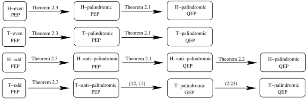
Theorem 2.3. If (2.25) is a even or a odd PEP, then (2.27) is a ?-palindromic or a ?-anti-?-palindromic PEP, respectively.
We illustrate the relations between various structured PEPs in Figure 2.1. From Figure 2.1, we see that T-even, T-odd, T-anti-palindromic and T-palindromic PEPs with even degree can be reduced to T-PQEPs. Thus, the structure-preserving methods in [7] can be used to solve the associated T-PQEPs. On the other hand, we see that H-even, H-odd, H-anti-palindromic and H-palindromic PEPs with even degree can be reduced to H-PQEPs. Therefore, it is motivated to develop a structure-preserving algorithm in the next section for solving the H-PQEP.
3. H-palindromic quadratic eigenvalue problems. Consider the H-PQEP
Q(λ)x ≡ (λ2AH1 + λA0+ A1)x = 0, (3.1)
where A1, A0 ∈ Cn×n with AH0 = A0. Taking the conjugate transpose of (3.1), we
easily see that the eigenvalues of Q(λ) have a ‘symplectic’ property, that is, they are
H−even PEP H−palindromic PEP T−even PEP PEP T−palindromic PEP H−anti−palindromic PEP H−palindromic QEP T−palindromic QEP H−anti−palindromic QEP H−palindromic QEP Theorem 2.3 Theorem 2.3 Theorem 2.1 Theorem 2.1 Theorem 2.1 Theorem 2.2 H−odd T−odd PEP Theorem 2.3 T−palindromic QEP T−palindromic GEP PEP Theorem 2.3 T−anti−palindromic [12, 13] (2.23)
Fig. 2.1. Relations between various structured PEPs.
paired with respect to the unit circle, containing both eigenvalues λ and its conjugate reciprocal 1/¯λ.
Classical linearizations of (3.1) in a companion form, generally, cannot preserve the symplectic structure. Fortunately, the special linearization of (3.1) (see [2] or [7])
(M − λL)z ≡ µ· A1 0 −A0 −I ¸ − λ · 0 I AH 1 0 ¸¶ · x y ¸ = 0 (3.2) satisfies MJ MH= LJ LH (3.3)
which preserves symplecticity, where J ≡ J2n is the 2n × 2n matrix
·
0 In
−In 0 ¸
. A pencil M − λL or the matrix pair (M, L) satisfying (3.3) is called H-symplectic.
For any real symplectic matrix pair (M, L) satisfying (3.3), a structure-preserving (S + S−1)-transform for the computation of all its eigenvalues was proposed by [9]. For a H-symplectic matrix pair (M, L), the (S + S−1)-transform (Ms, Ls) is defined by
Ms≡ MJ LH+ LJ MH≡ KJ , Ls≡ LJ LH ≡ N J . (3.4) It is easily seen that K and N are both complex conjugate skew-Hamiltonian, i.e.,
KJ = J KH and N J = J NH. Hence, if µ is an eigenvalue of (K, N ), so is ¯µ. We first give the relationship between eigenpairs of a H-symplectic matrix pair and its (S + S−1)-transform.
Theorem 3.1. Let (M, L) be H-symplectic and (Ms, Ls) be its (S + S−1
)-transform as in (3.4). Suppose zs is an eigenvector of (Ms, Ls) corresponding to
µ = ν +1
ν. If (LH−ν1MH)zs6= 0 or (LH− νMH)zs6= 0, then (ν, J (LH−1νMH)zs)
or (1/ν, J (LH− νMH)zs) is an eigenpair of (M, L).
Proof. As in [9], since MJ MH= LJ LH, by (3.4) it holds that 0 = [Ms− µLs] zs= · MJ LH+ LJ MH− (ν +1 ν)LJ L H ¸ zs = (M − νL)J (LH−1 νM H)zs (3.5a) = (M −1 νL)J (L H− νMH)zs. (3.5b) 10
By applying (3.5a), if (LH−1
νMH)zs6= 0, then J (LH−1νMH)zs is an eigenvector of (M, L) corresponding to ν. By applying (3.5b), if (LH − νMH)zs 6= 0, then
J (LH− νMH)zsis an eigenvector of (M, L) corresponding to 1/ν.
If (M, L) is of the form in (3.2), we give the relationship between eigenpairs of (Ms, Ls) and Q(λ) in the following theorem.
Theorem 3.2. Let (M, L) be H-symplectic of the form in (3.2) and (Ms, Ls)
be its (S + S−1)-transform. Suppose that the columns of Zs ≡ [ZT
s1, Zs2T]T with
Zs1, Zs2 ∈ Cn×p and p ≥ 1 form all linearly independent eigenvectors of (Ms, Ls)
corresponding to the eigenvalue µ 6= ±2. Let ν be a root of the quadratic equation λ +1
λ = µ. Then: (i) if rank(Zs1+1
νZs2) ≥ 1 and rank(Zs1+ νZs2) ≥ 1, then the linearly independent
columns of Zs1+1νZs2and Zs1+νZs2are eigenvectors of Q(λ) corresponding
to ν and 1
ν, respectively. Furthermore,
Null(Zs1+1
νZs2) ∩ Null(Zs1+ νZs2) = {0}. (3.6) Note that Null(B) denotes the null space of B; and
(ii) if Zs1+ νZs2 = 0, then the columns of Zs1+ 1
νZs2 are linearly independent
eigenvectors of Q(λ) corresponding to ν. Proof. (i). From (3.5a) and (3.5b), it follows that
(M − νL) · Zs1+ν1Zs2 Xν ¸ = 0 (3.7a) and (M −1 νL) · Zs1+ νZs2 X1/ν ¸ = 0 (3.7b) where Xν≡ 1 νA H 1Zs1− 1 νA0Zs2− A1Zs2, X1/ν ≡ νA H 1 Zs1− νA0Zs2− A1Zs2. (3.8) Since (M, L) is of the form in (3.2), from (3.7a), we have
Xν= 1 νA1(Zs1+ 1 νZs2) (3.9a) and A0(Zs1+1 νZs2) + Xν+ νA H 1 (Zs1+ 1 νZs2) = 0. (3.9b)
Substituting Xν in (3.9a) into (3.9b) and multiplying (3.9b) by ν we get
Q(ν)(Zs1+1
νZs2) = 0.
Similarly, from (3.7b), we have Q(1
ν)(Zs1+ νZs2) = 0.
To show (3.6), suppose that there is a U1 ∈ Cp×m with rank(U1) = m ≥ 1 such
that
(Zs1+1
νZs2)U1= 0 and (Zs1+ νZs2)U1= 0. (3.10) 11
This implies Zs1U1= Zs2U1= 0, i.e., ZsU1= 0. On the other hand, since Zsand U1
are of full rank, ZsU16= 0. This is a contradiction.
(ii) Since Zs1+ νZs2= 0, from (3.2) and (3.7b), it follows that X1/ν= 0.
There-fore, 1
ν is not an eigenvalue of (M, L) and Q(λ). We now show that Zs1+ 1
νZs2 is of full rank. Suppose not, i.e., there is a U1 ∈ Cp×m with rank(U 1) = m ≥ 1 such that µ Zs1+1 νZs2 ¶ U1= 0. (3.11)
Then, it holds that Zs1U1= −ν1Zs2U16= 0, because Zsand U1are of full rank. Since ν 6= ±1, we have Zs1U1+νZs2U1= (1−ν2)Zs1U16= 0. From (3.7b) it follows that the
nonzero columns of Zs1U1+νZs2U1are eigenvectors of Q(λ) corresponding toν1. This
is a contradiction, since 1
ν is not an eigenvalue of Q(λ). From (i) it follows that the columns of Zs1+1
νZs2form linearly independent eigenvectors of Q(λ) corresponding to ν.
Structure-Preserving Algorithm. In [7], a structure-preserving algorithm (SPA) based on Patel’s algorithm [14] has developed for solving T-PQEPs. In or-der to solve a H-PQEP, we apply the (S + S−1)-transform to the H-symplectic pair (M, L) of the form (3.2) and get the GEP
Kzs= µN zs, (3.12) where K = · A0 AH1 − A1 A1− AH1 A0 ¸ , N = · −A1 0 0 −AH 1 ¸ (3.13) are H-skew-Hamiltonian. However, Patel’s algorithm can only be used to solve (3.12) in the real case, but not be applied to solve (3.12) in the complex conjugate case directly. In the following, we shall convert (K, N ) in (3.13) into an enlarged real T-skew-Hamiltonian pair so that Patel’s algorithm can be applied.
Let
A0= A0R+ ıA0I, A1= A1R+ ıA1I,
where A0R, A0I, A1R, A1I ∈ Rn×n with AT0R= A0R and AT0I = −A0I. Then K and N
in (3.13) can be represented by K = · A0R AT1R− A1R A1R− AT1R A0R ¸ + ı · A0I −(A1I+ AT1I) A1I+ AT1I A0I ¸ ≡ KR+ ıKI (3.14) and N = · −A1R 0 0 −AT 1R ¸ + ı · −A1I 0 0 AT 1I ¸ ≡ NR+ ıNI. (3.15) We extend (K, N ) to a real 4n × 4n matrix pair (K2, N2) by
K2= · KR −KI KI KR ¸ and N2= · NR −NI NI NR ¸ ∈ R4n×4n. (3.16) 12
From (3.16) it is easily seen that if µ is an eigenvalue of (K, N ), then µ and ¯µ are
eigenvalues of (K2, N2).
Theorem 3.3. All eigenvalues of (K2, N2) are double.
Proof. Substituting matrices KR, KI, NR, NI in (3.14) and (3.15) into (3.16), we get K2= A0R AT1R− A1R −A0I A1I+ AT1I A1R− AT1R A0R −(A1I+ AT1I) −A0I A0I −(A1I + AT1I) A0R AT1R− A1R A1I+ AT1I A0I A1R− AT1R A0R and N2= −A1R 0 A1I 0 0 −AT 1R 0 −AT1I −A1I 0 −A1R 0 0 AT 1I 0 −AT1R . Define Π = diag{In, · 0 In In 0 ¸
, In}. Then it holds that
e K2≡ ΠK2Π = A0R −A0I AT1R− A1R A1I+ AT1I A0I A0R −(A1I+ AT1I) AT1R− A1R A1R− AT1R −(A1I+ AT1I) A0R −A0I A1I+ AT1I A1R− AT1R A0I A0R (3.17a) and e N2≡ ΠN2Π = −A1R A1I 0 0 −A1I −A1R 0 0 0 0 −AT 1R −AT1I 0 0 AT 1I −AT1R . (3.17b)
It is easy to check that eK2 and eN2 are real skew-Hamiltonian, i.e., ( eK2J4n)T = − eK2J4n and ( eN2J4n)T = − eN2J4n. Therefore, from the result of [9] it follows that
all eigenvalues of ( eK2, eN2) are double.
From (3.4), we see that µ is an eigenvalue of (K, N ) if and only if ¯µ is an eigenvalue
of (K, N ). The relationship between eigenpairs of (K, N ) and (K2, N2) is given in the
following theorem. Theorem 3.4.
(i) If (K, N ) has an eigenvalue α + ıβ associated with the eigenvector x + ıy, where
α, β ∈ R and x, y ∈ R2n, then · x y ¸ ± ı · y −x ¸ is an eigenvector of (K2, N2) corresponding to α ± ıβ.
(ii) If (K2, N2) has an eigenvalue α + ıβ associated with the eigenvector
· x1 x2 ¸ + ı · y1 y2 ¸
, then x + ıy is an eigenvector of (K, N ) corresponding to α + ıβ with x = x1− y2, y = x2+ y1.
Proof. (i) Since K(x + ıy) = (α + ıβ)N (x + ıy), comparing the real and the
imaginary parts of both sides, we come to
K2 µ· x y ¸ ± ı · y −x ¸¶ = (α ± ıβ)N2 µ· x y ¸ ± ı · y −x ¸¶ . (ii) Since · x1 x2 ¸ + ı · y1 y2 ¸ is an eigenvector of (K2, N2) corresponding to α + ıβ, it holds that KRx1− KIx2= α(NRx1− NIx2) − β(NRy1− NIy2), (3.18a) KRy1− KIy2= β(NRx1− NIx2) + α(NRy1− NIy2), (3.18b) KIx1+ KRx2= α(NIx1+ NRx2) − β(NIy1+ NRy2), (3.18c) KIy1+ KRy2= β(NIx1+ NRx2) + α(NIy1+ NRy2). (3.18d)
Set x = x1− y2and y = x2+ y1. Subtracting (3.18a) from (3.18d) and adding (3.18c)
and (3.18b), we get
KRx − KIy = α(NRx − NIy) − β(NIx + NRy), (3.19a)
KIx + KRy = β(NRx − NIy) + α(NIx + NRy). (3.19b) Thus, x + ıy is an eigenvector of (K, N ) corresponding to α + ıβ.
From Theorem 3.3 and Theorem 3.4, the eigenpairs of Kzs= µN zscan be com-puted from the eigenpairs of eK2z = µ e˜ N2z where e˜ K2 and eN2 are defined in (3.17).
Since eK2 and eN2 are both real skew-Hamiltonian, based on Patel’s approach [7, 14],
the pair ( eK2, eN2) can be reduced to block upper triangular forms
e K2:= QTKe2Z = · K11 K12 0 KT 11 ¸ , Ne2:= QTNe2Z = · N11 N12 0 NT 11 ¸ , (3.20)
where Q, Z ∈ R4n×4n are orthogonal satisfying
Q = J4nTZJ4n, (3.21)
and K11, N11∈ R2n×2n are upper Hessenberg and upper triangular, respectively.
From Theorem 3.3 and (3.20), we see that the pair (K11, N11) has the same
spectrum as ( eK2, eN2). We then apply the QZ algorithm to (K11, N11) for computing
all eigenpairs {(µj, ˜zj)}2n j=1. Consequently, {(µj, ΠZ · ˜ zj 0 ¸ )}2n j=1 are 2n eigenpairs of (K2, N2), where Π is defined in (3.17). Let µj= αj+ ıβj and
ΠZ · ˜ zj 0 ¸ ≡ · x1j x2j ¸ + ı · y1j y2j ¸
with αj, βj∈ R and x1j, x2j, y1j, y2j∈ R2n. From Theorem 3.4, {(αj+ ıβj, JT(x1j− y2j+ı(x2j+y1j)))}2nj=1are eigenpairs of (Ms, Ls). Finally, we compute all eigenvalues and the associated eigenvectors of Q(λ) by Theorem 3.2.
Algorithm 3.1 (Structure-Preserving Algorithm (SPA) for H-PQEP).
Input: A H-palindromic quadratic pencil Q(λ) ≡ λ2AH
1 + λA0+ A1 with A0, A1∈ Cn×n and AH0 = A0;
Output: All eigenvalues and eigenvectors of Q(λ). Step 1. Form the matrix pair ( eK2, eN2) as in (3.17);
Step 2. Reduce ( eK2, eN2) to block upper triangular forms as in (3.20); Step 3. Compute eigenpairs {(µj, ˜zj)}2nj=1 of (K11, N11) defined in (3.20)
by the QZ algorithm; Step 4. Compute ΠZ · ˜ zj 0 ¸ ≡ · x1j x2j ¸ + ı · y1j y2j ¸ , j = 1, 2, . . . , 2n;
Step 5. Compute the eigenpair (µj, zj), for j = 1, 2, . . . , 2n, of (Ms, Ls) by
zj = JT(x1j− y2j+ ı(x2j+ y1j)) ≡ [zj1T, zj2T]T;
Step 6. Compute νj and ν1j by solving ν2− µjν + 1 = 0;
Compute xj1≡ zj1+ν1jzj2 and xj2≡ zj1+ νjzj2for j = 1, 2, . . . , 2n;
Step 7. If xj1is a nonzero vector, then it is an eigenvector of Q(λ)
corresponding to νj; If xj2is a nonzero vector, then it is an eigenvector
of Q(λ) corresponding to 1
νj;
4. Backward error analysis. Let (λ, x) be an approximate eigenpair of a (?, ε)-palindromic polynomial pencil P(λ) in (1.1). We define the backward error of P(λ) by η(λ, x) := hP kP(λ)xk d j=1(|λ|d+j+ |λ|d−j) kAjk + |λ|dkA0k i kxk (4.1)
essentially as in [18]. For a (?, PPEP with degree 2d, Theorem 2.1 gives a (?, ε)-palindromic quadraticization Q(λ) ≡ λ2A?
1+ λA0+ A1 of the form (2.3) or (2.4).
Suppose (λ, y ≡ [yT
1, · · · , ydT]T) is an approximate eigenpair of Q(λ) associated with the residual r ≡ [rT
1, · · · , rdT]T. In what follows we shall study the relation between residuals r ≡ Q(λ)y and P2d(λ)y1.
For simplification, we first consider cases 2d = 8 and 10 with ε = 1. For 2d = 8: From (2.3) we have
λ2 A? 1 d?1A?4 A?3 0 0 0 d1I 0 0 0 0 −d? 2I d2I 0 0 0 + λ A0− I − A?4A4 0 A?2 0 0 −d1d?1I 0 0 A2 0 0 0 0 0 0 0 + A1 0 0 d?2I d1A4 0 0 0 A3 d?1I 0 0 0 0 −d2I 0 y1 y2 y3 y4 = r1 r2 r3 r4 , (4.2)
where d1 and d2are nonzero scalars. It follows that
r1= [λ2A?1+ λ(A0− I − A?4A4) + A1]y1+ λ2A4?d?1y2+ (λ2A?3+ λA?2)y3+ d?2y4, (4.3a) r2= d1A4y1− λd1d?1y2+ λ2d1y3, (4.3b) r3= (λA2+ A3)y1+ d?1y2− λ2d?2y4, (4.3c) r4= λ2d2y1− d2y3. (4.3d) 15
Then we have y3= λ2y1− d−12 r4, (4.4a) d? 1y2= 1 λ(λ 4I + A 4)y1− λd−12 r4−1 λd −1 1 r2, (4.4b) d?2y4= 1 λ3(λ 4I + λ2A 2+ λA3+ A4)y1−1 λd −1 2 r4− 1 λ3d −1 1 r2− 1 λ2r3. (4.4c)
Substituting (4.4) into (4.3a) we get
P8(λ)y1= d−11 (λ4A?4+ I)r2+ λ2d−12 (λ4A?4+ λ3A?3+ λ2A?2+ I)r4+ λr3+ λ3r1. (4.5)
For 2d = 10: From (2.4) we have λ 2 A? 1 A?5 0 A?3 0 0 0 −d? 1I 0 0 0 0 0 d1I 0 0 0 0 0 −d? 2I d2I 0 0 0 0 + λ A0 A?4 0 A?2 0 A4 0 0 0 0 0 0 0 0 0 A2 0 0 0 0 0 0 0 0 0 + A1 0 0 0 d?2I A5 0 0 0 0 0 −d1I 0 0 0 A3 0 d?1I 0 0 0 0 0 −d2I 0 y1 y2 y3 y4 y5 = r1 r2 r3 r4 r5 , (4.6)
where d1 and d2are nonzero scalars. It follows that
r1= (λ2A?1+ λA0+ A1)y1+ (λ2A?5+ λA?4)y2+ (λ2A?3+ λA?2)y4+ d?2y5, (4.7a)
r2= (λA4+ A5)y1− λ2d?1y3, (4.7b) r3= λ2d1y4− d1y2, (4.7c) r4= (λA2+ A3)y1+ d?1y3− λ2d?2y5, (4.7d) r5= λ2d2y1− d2y4. (4.7e) Then we have y4= λ2y1− d−12 r5, (4.8a) y2= λ4y1− λ2d2−1r5− d−11 r3, (4.8b) d? 1y3= 1 λ2(λA4+ A5)y1− 1 λ2r2, (4.8c) d? 2y5= 1 λ4(λ 3A 2+ λ2A3+ λA4+ A5)y1− 1 λ4r2− 1 λ2r4. (4.8d)
Substituting (4.8) into (4.7a), we get
P10(λ)y1= λ5d−12 (λ3A?5+ λ2A?4+ λA?3+ A?2)r5+ λ5d−11 (λA?5+ A?4)r3
+(λ4r
1+ λ2r4+ r2). (4.9)
In general, for 2d = 4m and 4m + 2 we have the following theorem. Theorem 4.1. Let (λ, y ≡ [yT
1, · · · , ydT]T) be an approximate eigenpair of (2.1)
associated with residual r ≡ [rT
1, · · · , rdT]T. Then
(i) for 2d = 4m, we have P4m(λ)y1= m−1X i=0 λ2id−1 i+1 2i X j=0 λ2m−jA? 2m−j+ √ εI r2i+2 +λ2m−1 m−1X i=1 λ−2ir 2m−2i+1+ λ2m−1r1≡ ˜r0; (4.10)
(ii) for 2d = 4m + 2, we have
P4m+2(λ)y1= λ2m+1 m X j=1 d−1 j 2m X i=2m−2j+1 λi−2m+2j−1A? i+1 rj+1 + m X i=1 λ2i−2r 2i+ λ2mr1≡ ˜r2. (4.11)
Proof. (A sketch) For both cases we consider the equation
(λ2A?
1+ A0+ A1)y = r, (4.12)
where A0 and A1 are given in (2.3) or (2.4). Let y ≡ [y1T, · · · , ydT]T and r ≡ [rT
1, · · · , rdT]T. As in the derivation of (4.5) and (4.9) we first derive the represen-tations of y2, . . . , yd by {ri}di=2 and y1 from the second to the last equations of (4.12).
Then, substituting y2, . . . , yd into the first equation of (4.12) and arranging the suit-able terms carefully, we get (4.10) and (4.11). Here we omit the details. A tedious proof can be found in Appendix.
On the other hand, suppose (ˆλ, ˆy) with ˆy = [ˆyT
1, · · · , ˆy2dT]T is an approximate
eigenpair of (1.2) with ε = 1 and ˆr = [ˆr1, · · · , ˆrT2d]T is the associated residual. That
is, Ad 0 · · · 0 0 −In .. . . .. 0 −In + ˆλ Ad−1 · · · A0 · · · A?d In 0 .. . . .. ... .. . . .. ... 0 · · · · · · In 0 ˆ y1 ˆ y2 .. . ˆ y2d = ˆ r1 ˆ r2 .. . ˆ r2d . (4.13) After computation, we also have the following theorem.
Theorem 4.2. Let (ˆλ, ˆy) be an approximate eigenpair of (1.2) associated with the residual ˆr satisfying (4.13). Then it holds
P2d(ˆλ)ˆy1= ˆr1− d−2 X k=0 Ak d−k X j=2 λd−k−j+1rˆ j− d X k=1 A? k d+k X j=2 ˆ λd+k−j+1rˆ j. (4.14)
In the following, we shall analyze the backward error of the structured lineariza-tion (λZ?+ Z)y = 0 proposed in [12]. If (λ, [λ2d−1xT, λ2d−2xT, · · · , λxT, xT]T) is an
eigenpair of λZ?+ Z , then (λZ?+ Z) λ2d−1x λ2d−2x .. . λx x = P2d(λ)x 0 .. . 0 P2d(λ)x = 0. (4.15)
Thus, (λ, x) is an eigenpair of P2d(λ). For simplification, we consider that 2d = 6.
Then Z?= A? 3 A?2− A3 A?1 A0 A1 A2 0 A? 3− A2 A?2− A3 A?1 A0 A1 0 −A1 A?3− A2 A?2− A3 A?1 A0 0 −A0 −A1 A?3− A2 A?2− A3 A?1 0 −A? 1 −A0 −A1 A?3− A2 A?2− A3 A? 3 0 0 0 0 A?3 .
Let (˜λ, ˜y) be an approximate eigenpair of (λZ?+ Z)y = 0 associated with the residual ˜
r, i.e.,
(˜λZ?+ Z)˜y = ˜r. (4.16)
From (4.16) it follows that ˜ r1= ˜λ [A?3y˜1+ (A?2− A3)˜y2+ A?1y˜3+ A0y˜4+ A1y˜5+ A2y˜6] + A3y˜1+ A3y˜6,(4.17a) ˜ r2= ˜λ [(A?3− A2)˜y2+ (A?2− A3)˜y3+ A1?y˜4+ A0y˜5+ A1y˜6] +(A2− A?3)˜y1+ (A3− A?2)˜y2− A?1y˜3− A0y˜4− A1y˜5, (4.17b) ˜ r3= ˜λ [−A1y˜2+ (A?3− A2)˜y3+ (A2?− A3)˜y4+ A?1y˜5+ A0y˜6] +A1y˜1+ (A2− A?3)˜y2+ (A3− A2?)˜y3− A?1y˜4− A0y˜5, (4.17c) ˜ r4= ˜λ [−A0y˜2− A1y˜3+ (A?3− A2)˜y4+ (A?2− A3)˜y5+ A?1y˜6] +A0y˜1+ A1y˜2+ (A2− A?3)˜y3+ (A3− A?2)˜y4− A?1y5, (4.17d) ˜ r5= ˜λ [−A?1y˜2− A0y˜3− A1y˜4+ (A?3− A2)˜y5+ (A?2− A3)˜y6] +A1?y˜1+ A0y˜2+ A1y˜3+ (A2− A?3)˜y4+ (A3− A?2)˜y5, (4.17e) ˜ r6= ˜λ [A?3y˜1+ A?3y˜6] + A?2y˜1+ A?1y˜2+ A0y˜3+ A1y˜4+ (A2− A?3)˜y5+ A3y˜6.(4.17f)
Multiplying (4.17b), (4.17c), (4.17d), (4.17e) and (4.17f) by ˜λ, ˜λ2, ˜λ3, ˜λ4 and ˜λ5,
respectively, and adding them to (4.17a), we get
P6(˜λ)(˜y1+ ˜y6) = 6 X i=1 ˜ λi−1r˜i.
In general, we have the following theorem.
Theorem 4.3. Suppose (4.15) holds and let (˜λ, [˜yT
1, · · · , ˜yT2d]T) be an approximate eigenpair of (λZ?+ Z)y = 0 associated with the residual [˜rT
1, · · · , ˜r2dT]T. Then P2d(˜λ)(˜y1+ ˜y2d) = 2d X i=1 ˜ λi−1r˜ i. 18
Remark 4.1. From Theorem 4.1 we see that the residual P2d(λ)y1 derived from the residual r = Q(λ)y of the quadraticization Q(λ) depends on the norms of A2, · · · , Ad, but is independent of the norms of A0 and A1. On the other hand, from Theorem 4.2 the residual P2d(ˆλ)ˆy1 derived from the residual ˆr = L(ˆλ)ˆy of the linearization L(ˆλ) depends on the norms of A0, A1, · · · , Ad. Generally, if the norms
of A0 and A1 are much dominant to the norms of A2, · · · , Ad, then the norms of
P2d(λ)y1 should be much smaller than that of P2d(ˆλ)ˆy1.
5. Balancing for PPEP and PQEP. Scaling is a commonly used technique for standard eigenvalue problems to improve the sensitivity of the eigenvalues. In this section, we shall discuss the diagonal scaling of the PPEP (1.1). In addition, the free parameters d1, . . . , dm in (2.3) and (2.4) will be chosen so as to scale the PPEP so that the backward errors of the eigenpairs for the PPEP will be improved. The discussed strategy for scaling, deduced from our numerical experiments, are not be unique or optimal.
First, consider the diagonal scaling of the PPEP (1.1). In order to balance the entries of coefficient matrices in the PPEP, we define a complex diagonal matrix
D ≡ diag(2α1, 2α2+ıβ2, · · · , 2αn+ıβn)
with αi, βi∈ R so that the magnitude of the entries of coefficient matrices in the new PPEP D d−1X j=0 λ2d−jA?d−j+ λdA0+ ε d X j=1 λd−jAj D?x = 0˜
are close to one as much as possible. That is, we shall determine α1, . . . , αn and
β2, . . . , βn so that
2αj+ıβja(k)
j` 2α`−ıβ` ≈ 1, (5.1)
for j, ` = 1, 2, . . . , n and k = 0, 1, . . . , d, where a(k)j` is the (j, `)-th entry of Ak. By taking logarithm of (5.1), the parameters, α1, . . . , αnand β2, . . . , βncan be determined by solving the least square problems
αj+ α`= −Re(log2(a(k)j`)) and βj− β`= −Im(log2(a(k)j` )),
where Re(c) and Im(c) represent the real and the imaginary parts of c, respectively. Then, {α1, . . . , αn} is solved by the normal equation
ATA α1 .. . αn = ATa
where a is the vector formed by −Re(log2(a(k)j` )), the nonzero entries of A are equal to 1 or 2 and ATA ≡ [a ij] with aij= ½ 4(d + 1) + (2d + 1)(n − 1), if i = j, 2d + 1, if i 6= j. 19
Furthermore, ATA is invertible and (ATA)−1≡ [ˆa ij] with ˆaij= ½ (4dn + 2n − 2d + 1)/δ, if i = j, −(2d + 1)/δ, if i 6= j, where δ = a2 11+ (n − 2)a11a12− (n − 1)a2126= 0.
Similarly, {β2, . . . , βn} is solved by the normal equation
BTB β2 .. . βn = BTb
where b is the vector formed by −Im(log2(a(k)j`)), the nonzero entries of B are equal to 1 or −1 and (BTB)−1 ≡ [ˆbij] with
ˆbij= ½
2/(n(2d + 1)), if i = j, 1/(n(2d + 1)), if i 6= j. It only requires O(n2) flops to determine the diagonal matrix D.
Next, we shall determine d1, . . . , dmin (2.3) and (2.4). Let
η(1)i = max{max{kA2m−jk1; j = 0, 1, . . . , 2i − 2}, 1} (for 2d = 4m), η(2)i = max{max{kA2m−j+1k1; j = 0, 1, . . . , 2i − 1}, 1} (for2d = 4m + 2),
for i = 1, 2, . . . , m. If we take di = η(1)i and di= η(2)i for i = 1, 2, . . . , m in (2.3) and (2.4), respectively, then from Theorem 4.1, we have
kP4m(λ)y1k∞≤ m−1X i=0 |λ|2i 2i X j=0 |λ|2m−j+ 1 kr2i+2k∞ +|λ|2m−1 m−1X i=1 |λ|−2ikr2m−2i+1k∞+ |λ|2m−1kr1k∞ and kP4m+2(λ)y1k∞≤ |λ|2m+1 m X j=1 X2m i=2m−2j+1 |λ|i−2m+2j−1 krj+1k∞ + m X i=1 |λ|2i−2kr 2ik∞+ |λ|2mkr1k∞
which imply that the upper bound of the residual P2d(λ)y1 is independent of the
norms of A0, . . . , Ad. However, such a choice for {di} may destroy the balance of the
coefficient matrices in (2.3) and (2.4) for the PQEP.
In order to balance dk = η(`)k and the entries of A2m−2k+1(k = 1, . . . , m − 1) as
well as dm= η(`)m and the entries of A1 for A1 in (2.3) and (2.4), we re-set dk = ξ(`)k
with ξ(`)k = v u u u tη(`)k Xn i=1 n X j=1 |A2m−2k+1(i, j)|/n2 , k = 1, . . . , m − 1, ξ(`)m = v u u u tη(`)m n X i=1 n X j=1 |A1(i, j)|/n2 ,
for ` = 1, 2. Here Ak(i, j) represents the (i, j)-th entry of Ak.
To balance the entries of A0and A1 in (2.3) and (2.4), we define
τ(1)= max 0≤k≤dmax n X i=1 n X j=1 |Ak(i, j)|/n2 , n X i=1 n X j=1 | ˜A0(i, j)|/n2, ρ(1) , τ(2)= max 0≤k≤dmax n X i=1 n X j=1 |Ak(i, j)|/n2 , ρ (2) , where ˜A0= A0− √ εI −√εA? 2mA2mand ρ(`)= max{ξk(`); k = 1, . . . , m}, for ` = 1, 2. We take dk= %(`)= p ρ(`)τ(`), for k = 1, . . . , m, ` = 1, 2.
Finally, for the case 2d = 4m, −√εd2
1I is a submatrix of A0in (2.3). In order to
balance this submatrix with other submatrices in A0, we let
χ = max max n X i=1 n X j=1 |A2k(i, j)|/n2; k = 1, . . . , m − 1 , n X i=1 n X j=1 | ˜A0(i, j)|/n2 , and modify d1 by d1= ( ¡ %(1)¢1/1.5, if χ <¡%(1)¢2, %(1), otherwise.
6. Numerical results. A standard approach for solving the (?, ε)-PPEP (1.1) is to transform it to a 2dn×2dn linear eigenvalue problem and compute the eigenpairs by the QZ algorithm. In this paper, we have proposed a structured quadraticization to transform (1.1) into a dn × dn PQEP, to which we apply the SPA (Algorithm 3.1). In this section, we compare the computational costs of these two approaches. Moreover, we also compare the backward errors and symplectic reciprocities of the eigenpairs from the SPA and QZ approaches as well as the direct application of “polyeig” in MATLAB on the (?, ε)-PPEP (1.1).
6.1. Computational cost. For a more efficient SPA, we reorder the submatrices in the matrix pair ( eK2, eN2) of (3.17) by the permutation matrices
Π1= In 0 0 0 0 0 0 I(d−1)n 0 0 0 0 0 0 I(d−2)n 0 0 0 In 0 0 In 0 0 0 , Π2= 0 0 In 0 0 0 0 I(d−2)n 0 0 0 0 0 0 0 0 0 In 0 0 0 0 I(d−2)n 0 0 0 0 In 0 0 In 0 0 0 0 0 .
For the case 2d = 4m, we substitute A1 of (2.3a) into eN2of (3.17b), and get
e N2:= · Π1 0 0 Π2 ¸ e N2 · ΠT 2 0 0 ΠT 1 ¸ = D11 0 −V11 V21 0 D11 V21 V11 0 0 − ˜A2m,R − ˜A2m,I 0 0 A˜2m,I − ˜A2m,R ⊕ D11 0 0 0 0 D11 0 0 −VT 11 V21T − ˜AT2m,R A˜T2m,I VT 21 V11T − ˜AT2m,I − ˜AT2m,R , where D11= diag ¡ −dmIn −d1In εd2In −d2I εd3I · · · −dm−1In εdmIn ¢ , VT 11= £ −AT
1,I −AT2m−1,I 0 · · · −AT3,I 0
¤ , VT 21= £ −AT 1,R −AT2m−1,R 0 · · · −AT3,R 0 ¤ , ˜ A2m= ε √ εd1A2m.
Here Ak,Rand Ak,I represent the real and the imaginary parts of Ak. Similarly, for the case 2d = 4m + 2, we have
e N2:= · Π1 0 0 Π2 ¸ e N2 · ΠT 2 0 0 ΠT 1 ¸ = D12 0 −V12 V22 0 D12 V22 V12
0 0 −A2m+1,R −A2m+1,I
0 0 A2m+1,I −A2m+1,R ⊕ D12 0 0 0 0 D12 0 0 −VT 12 V22T −AT2m+1,R AT2m+1,I VT
22 V12T −AT2m+1,I −AT2m+1,R
, where D12= diag ¡ −dmIn εd1In −d1In εd2In −d2In · · · −dm−1In εdmIn ¢ , VT 12= £ −AT
1,I 0 −AT2m−1,I 0 · · · −AT3,I 0
¤ , VT 22= £ −AT 1,R 0 −AT2m−1,R 0 · · · −AT3,R 0 ¤ . Set e K2:= · Π1 0 0 Π2 ¸ e K2 · ΠT 2 0 0 ΠT 1 ¸ .
Now, we use the following steps to reduce the new pair ( eK2, eN2) to block upper
triangular forms as in (3.20):
• (QR factorization and updating with real arithmetic operations) Compute Q1 and Z1 such that QT1Ne2Z1 =
"
N11(1) 0 0 (N11(1))T
#
, where N11(1) is upper triangular. In this step, it requires 32/3n3 flops for the QR factorization of
an 2n × 2n real matrix and 48dn3+ 24dn2 flops to update QT
1Ke2Z1.
• (Given’s rotations and updating with real arithmetic operations) For each j-th columns of ( eK2, eN2) with j = 1, . . . , 2dn − 2, we need to
(i) annihilate eK2(2nd+i, j) and eK2(2nd+j, i) with i > j by using rotations of
the (2nd+i+1, j)-th and (2nd+i, j)-th entries, and the (2nd+j, i+1)-th and (2nd + j, i)-th entries of eK2, respectively. It requires 6(4dn − j) + 5
flops. Updating the corresponding rows and columns of eN2 requires
6(i + 1) flops. Subsequently, annihilating the corresponding fill-in for e
N2 by Given’s rotations requires 6(2dn − i) + 5 flops. Updating the
corresponding matrix eK2 requires 6(4dn − j + 1) flops. Consequently,
annihilating the entries from 2nd + j + 1 to 4dn − 1 in the j-th column of e
K2and preserving the upper triangular N11(1)require (2dn−j −2)(60dn−
12j + 22) flops.
(ii) annihilate eK2(4dn, j) and eK2(2dn + j, 2nd) by using the rotation of the
(2nd, j)-th and (4nd, j)-th entries, (2nd+j, 4nd)-th and (2nd+j, 2nd)-th entries of eK2, respectively, and update eN2 which require 6(4dn − j) +
5 + 6(2dn) flops.
(iii) annihilate eK2(i, j) and eK2(2nd + j, 2nd + i) with i > j + 1 by using the
rotations of (i − 1, j)-th and (i, j)-th entries, (2nd + j, 2nd + i − 1)-th and (2nd + j, 2nd + i)-th entries of of eK2, respectively. It requires 6(4dn − j) + 5. Updating the corresponding rows and columns of eN2 requires
6(4nd − i + 2) flops. On the other hand, annihilating the corresponding filled in for eN2by using Given’s rotations requires 6i + 5 flops.
Updat-ing the correspondUpdat-ing matrix eK2 needs 6(4dn − j) flops. Consequently,
annihilating the entries from 2nd to j + 2 of the j-th column for eK2and
preserving the upper triangular N11(1)require (2dn−j−1)(72dn−12j+22) flops.
From above steps, we see that reducing the pair ( eK2, eN2) in (3.17) to block upper
triangular forms of (3.20) requires
48dn3+ 24dn2+ 2dn−2X j=1 £ 264d2n2− (180j + 68)dn + 24j2− 14j − 61¤ = (232d3+ 48d)n3− (296d2− 24d)n2− 20dn + 84 flops.
The QZ step for the real upper Hessenberg and triangular pair (K11, N11) in (3.20)
requires 22(2dn)3= 176d3n3flops to obtain the upper quasi-triangular and triangular
pair, i.e., all eigenvalues of (K11, N11). Computing the corresponding eigenvectors
by using inverse power method requires 4 × (2dn) × (2dn)2 = 32d3n3 flops. The
eigenvectors of ( eK2, eN2) can be computed by an additional (376d3+32d)n3−(332d2−
16d)n2+56dn flops. Therefore, computed all eigenvalues of ( eK
2, eN2) requires (408d3+
48d)n3− (1400d2− 24d)n2flops, and an additional (408d3+ 32d)n3− (332d2− 16d)n2
flops are required for the corresponding eigenvectors. For the QZ algorithm applied to a 2dn×2dn palindromic linearization λZ +Z∗, it requires approximately 120(2dn)3=
Eigenvalues Eigenvectors Total Algorithm 3.1 (408d3+ 48d)n3 (408d3+ 32d)n3 (816d3+ 80d)n3
QZ algorithm 960d3n3 736d3n3 1696d3n3
Table 6.1
Computational flops of Algorithm 3.1 and QZ algorithm on (Z?, −Z).
960d3n3 flops for the eigenvalues and an additional 92(2dn)3= 736d3n3 flops for the
eigenvectors.
We summarize the computational flops of Algorithm 3.1 and the QZ algorithm in Table 6.1
6.2. Numerical experiments. In Sections 2 and 3, we propose a structured quadraticization to transform a PPEP into a PQEP, to which we apply Algorithm 3.1 (SPA). Here, we use “SQ SPA” to denote the proposed method. We use “SL QZ” to denote the method asscoiated with the structured linearization (λZ?+ Z)y = 0, proposed in [12] for the PPEP, to which the QZ algorithm is applied. In the following, we show the numerical comparisons of the backward errors and symplectic reciprocities of eigenpairs, computed by SQ SPA, “polyeig” in MATLAB (applied directly to (1.1)) and SL QZ.
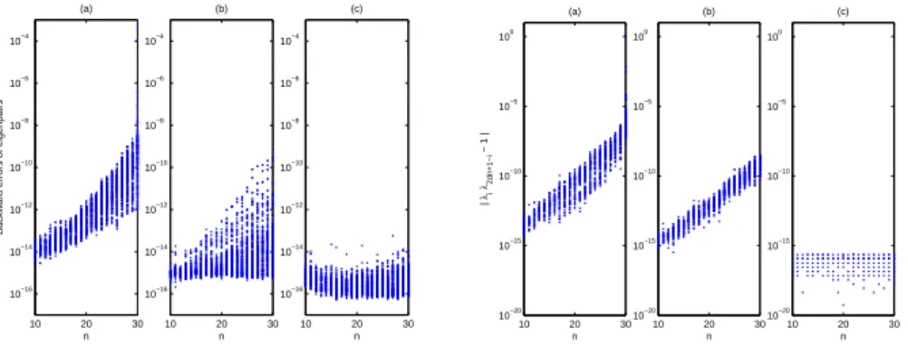
As mentioned before, theoretically, the eigenvalues of H-PPEP appear in recipro-cal pairs (λ, 1/¯λ). So, if we sort the eigenvalues in ascending order by modulus, the
product of the i-th eigenvalue and the conjugate of the (2dn + 1 − i)-th eigenvalue should be one. Therefore, we define the reciprocities of computed eigenvalues by
ri≡ |λi¯λ2dn+1−i− 1|, i = 1, . . . , dn. (6.1)
All numerical experiments are carried out using MATLAB 2008a with the machine precision eps ≈ 2.22 × 10⁻¹⁶.
Let Cn,m,rdenote the set of random complex n × m matrices with normal distri-bution which real and imaginary parts of the entries in [−r, r].
Example 6.1. Consider the discrete-time optimal control problem
min {uj} ∞ X j=0 · xj uj ¸H· Q S SH R ¸ · xj uj ¸
with QH = Q, Mi ∈ Cn×n, S, B ∈ Cn×m and RH = R ∈ Cm×m subject to the
discrete-time control
2d
X i=0
Mixi+d= Bui
for given x0, x1, · · · , x2d−1. This system corresponds to a H-palindromic polyno-24
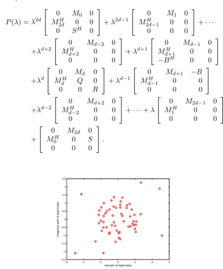
mial [1, 10] P (λ) = λ2d M0H M0 0 2d 0 0 0 SH 0 + λ2d−1 MH0 M1 0 2d−1 0 0 0 0 0 + · · · +λd+2 M0H Md−2 0 d+2 0 0 0 0 0 + λd+1 M0H Md−1 0 d+1 0 0 −BH 0 0 +λd M0H Md 0 d Q 0 0 0 R + λd−1 M0H Md+1 −B d−1 0 0 0 0 0 +λd−2 M0H Md+2 0 d−2 0 0 0 0 0 + · · · + λ M0H M2d−1 0 1 0 0 0 0 0 + M0H M2d 0 0 0 S 0 0 0 . −3 −2 −1 0 1 2 3 −2.5 −2 −1.5 −1 −0.5 0 0.5 1 1.5 2 2.5
real part of eigenvalue
imaginary part of eigenvalue
Fig. 6.1. The distribution of nonzero finite eigenvalues of Example 6.1.
Take n = 5, m = 1 , d = 3, and Q, Mi ∈ Cn,n,10, S, B ∈ Cn,m,10 and R ∈
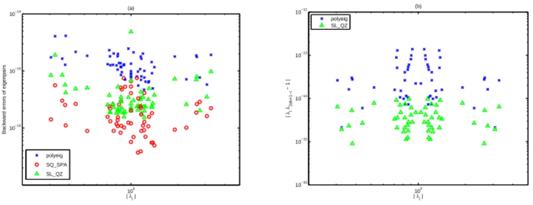
Cm,m,10. The corresponding nonzero finite eigenvalues are shown in Figure 6.1. The H-palindromic PEP has infinite and zero eigenvalues which can be computed by the SQ SPA and polyeig, but not by the SL QZ. For the SL QZ, the eigenvalue nearest zero is |λ| = 4.4 × 10⁻⁶. The backward errors and symplectic reciprocities ri of the eigenpairs are shown in Figure 6.2 (a) and (b). We use the notations “×”, “4” and “o” to denote the results computed by the polyeig, SL QZ and SQ SPA, respectively, and some zero reciprocity riof the eigenpairs produced by the SQ SPA are not shown. From Figure 6.1, we see that the SQ SPA not only preserve the reciprocal property of the eigenvalues but also provides better accuracy than that by the polyeig and SL QZ. In the following, we construct three examples with higher degrees and larger matrix sizes than that of Example 6.1.
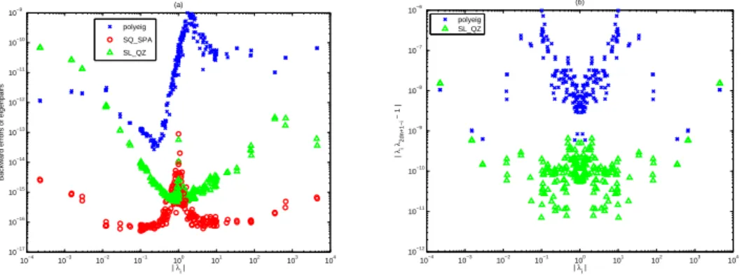
Example 6.2. Consider the H-palindromic PEP with d = 5 and Ai ∈ Cn,n,100
for i = 0, . . . , 5.
Example 6.3. Consider the H-palindromic PEP with d = 4, A1, A3, A4 ∈ 25