BAYES ANALYSIS FOR FAULT LOCATION IN DISTRIBUTED SYSTEMS

IEEE TRANSACTIONS ON RELIABILITY, VOL. 43, NO. 3, 1994 SEPTEMBER 45 7

Bayes Analysis for Fault Location in Distributed Systems

Yu Lo Cyrus Chang, Member IEEE

Leslie C. Lander,

Associate

Member IEEE

The

University

of

Tennessee, Chattanooga

State

University

of

New

York, Binghamton

National

Chiao Tung

University,

Hsinchu

Come11 University,

Ithaca

HOmg-Shing LU

Martin

T.

Wells

Keywords

-

Bayes analysis, Distance measure, Fault location,

Less function, Comparison test, Probabilistic comparison model, System diagnosis.

Reader Aids

-

General purpose: Advance state of the art

Special math needed for explanations: Bayes statistics Special math needed to use the results Same Results useful to: Reliability & test analysts

Summary & Conclusions

-

We propose a simple & practical probabilistic model, using multiple incomplete test concepts, for fault location in distributed systems using a Bayes analysis pro- cedure. S i c e it is easier to compare test results among processing units, our model is comparison-based. This approach is realistic & complete in the sense that it does not assume conditions such as permanently faulty units, complete tests, and perfect or non- nuhaous environments. It can handle, without any overhead, fault- free systems so that the test procedure can be used to monitor a functioning system. Given a system S with a specific test graph, the corresponding conditional distribution between the comparison test results (syndrome) and the fault patterns of S can be generated. To avoid the complex global Bayes estimation process, we develop a simple bitwise Bayes algorithm for fault location of S, which locates system failures with linear complexity, making it suitable for hard real-time systems. Hence, our approach is appealing both

from the practical & theoretical points of view.

. .

1. INTRODUCTION

This paper studies fault location using Bayes inference methods based on a simple probabilistic comparison model. The distributed systems under consideration consist of a collection of units (subsystems) connected through a network that distributes data and, possibly, processes throughout the system.

Our approach provides a generalized solution to the randomiz- ed fault diagnosis problem. Previous research has highlighted & studied individual obstacles in the faultdiagnosis process. Those obstacles are:

System diagnosis results might only be valid if the fraction of faulty units has a restrictive upper bound [36]. System can have non-permanent faults [26].

Faulty units can behave maliciously and lie about their results u71.

Tests might be incomplete [31,32].

For some test strategies, faulty units have to be assumed to be still able to execute assigned tests [30].

There might be noisy environments or errors in transmit- ting/receiving devices [5].

The probability of failure can vary as the run-time advances

[91. 4

Probabilistic methods can cope with this list of effects; and important advances have been made in the past few years [1,3-13,15,20-22,371. Indeed, the listed randomizing effects might indicate that this approach is more realistic than a deter- ministic one. However, a general probabilistic approach in earlier papers involved a drastic increase in computational com- plexity. The idea of using comparison testing appeared in [14, 251, and was combined with the probabilistic approach in [ 15, 16,211. Comparison-based testing is used because it is less in- trusive [ 151 than having the system units devote processing time to testing & evaluating each other. We have shown [8,10] that linear complexity can be achieved both by: 1) our bitwise Bayes

(BWB') algorithm based on the decision theoretic approach, and 2) a heuristic algorithm when performing classical point estimation. The BWB fault-location algorithm handles any number of faults in the same way; therefore it can diagnose a fault-free system as well as a system with many faulty units. The BWB algorithm accounts for the probability of unit failure [24] and incorporates the change of that probability as opera- tion time increases. Explicit inclusion of the probability of failure of a unit is also used in [3, 4, 221, although they assume the probability is constant. Most of the other fault-location research developed for multiprocessor systems more or less resembles the concepts developed by the Preparata, Metze, Chien (PMC) model [30]. The main reason for this similarity is that the same set of simplifying assumptions tends to be repeated, the limita- tions of which are in [15]. Other approaches can be found in [3-5,17,18,22,23,30,33,35,36], including work for general multiprocessor systems.

The model for testing a system with n units involves distributing a set of tests to the units, observing the results of

the tests, and running a diagnosis algorithm to locate faulty wits.

The BWB algorithm is 0 ( n)

,

making it interesting for hard real- time applications. The simplicity of the BWB depends on decom- posing the system (global) b y e s estimation into a bit-wise Bayes estimation by introducing a loss function. None of the data gathered from the tests has to be discarded. The chosen loss function is an admissible' Bayes decision rule [2] for fault location, which gives theoretical support to the approach. Some simulation results are discussed in section 5 .

'The BWB algorithm is called the B-algorithm in [6, 7, 11-13].

'Admissible implies that there is no decision rule with smaller risk function [2: p lo].

458 IEEE TRANSACTIONS ON RELIABILITY, VOL. 43, NO. 3, 1994 SEPTEMBER

Acronym-’

B W B

bit-wise Bayes (algorithm) HPD highest posterior density LT likelihood table

UUT unit under test.

Notation

S system name

n

G ( U , E ) an undirected test graph with vertex set

U

and edge number of units in S

-

-set E

{U& k = 0, 1 , 2 ,

...,

n - 1 } : vertex set of n units of S

{ (ui, uj): ui, uj E

U):

edge set of m comparison assignments of the UUT from S

9 (U, is faulty)

4)n-2

. . .

40:

(system) fault pattern of the n units

3

=

4,,n-~

4,,,-2

...4,,0

: fault status of U, when the fault pattern of S is

{90,+l,.

.

.

,+y- : set of all possible fault patterns of S. The are enumerated SO that

4j,n-1

4j,n-2

...

4j,o

is the binary representation o f j , possibly with leading O’s, eg, cp6 = 0110 in a 4-unit system

individual test task i that can be applied to S {tl, t2,

...,

t p } : test4 consisting o f p tasks ti number of tests in a sequence

{ T ( @ : k = 1 , 2 ,

. .

.

, T } : sequence of r tests, each T ( k )

represents a test T

S(the results of applying T to ui & uj disagreellink 1 connects ui & uj): 1 = 0, 1 , 2 ,

...

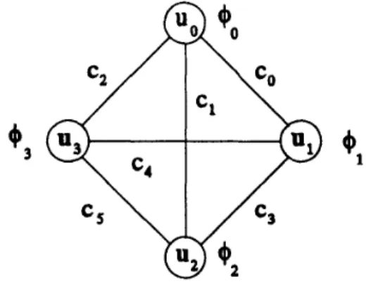
m-1; eg, figure

1 shows a complete graph of n = 4 units, and m = (;) =

(4)

links

c,,,-~ c , - ~

.

..

co: global (system) comparison pattern of the m links

comparison result of test T ( , )

{Co,Cl,...,C2m-l}:

set of all comparison patterns. The

Ci

are enumerated so that if

Ci

= cmPl cmF2

.

. .

co. then c,-~ cm-g

...

co is the binary representation of i. wssiblv with leading 0’s

C ( l j k(2)

..I

C ( T ) . Y

c“..

. J )

Other, standard notation is given in “Information for Readers & Authors” at the rear of each issue.

2 . PROBABILISTIC COMPARISON-BASED MODEL Assumptions

simultaneously.

1. System S has n units; several units can be faulty

’ m e singular / plural of an acronym are always spelled the same. 4A rest is a procedure for identifying whether a UUT is behaving nor- mally or abnormally

-

in the comparison model

-

by means of the value it returns.

3

Q,

Figure 1. 4-Unit System with Complete Test-Graph

2 . The faults in S are identified by a fault pattern

3.

Each fault pattern +j E 0 is possible in S.

3. Individual tests T can be incomplete in the sense that they need not always cause a faulty unit to return an incorrect result.

4. T(’) & T(,’) can be replications or can include different tasks belonging to the same class.

5 . Sequences Tare applied periodically to S.

T

generates

a sequence of T comparison patterns

{ c ‘ ~ ’

E 9, k =

1,2,.

.

.

,T} ; this sequence is analyzed probabilistically to deter-

mine the faulty units. 4 Let cl connect ui & uj. The behavior of the Comparison test of ui & uj can be characterized & modeled using the following conditional probability test parameters:

p l =

Pr

{ q =

0

I

c$i =

4j

= 0} :

Pr

{agreement between fault-free units},

ql =

Pr

{q= 1

1

+i

# + j } : Pr {disagreement between a faulty and a fault-free unit},

rl = Pr {cl= 1

I 4i

=

4j =

l } : Pr {disagreement between faulty units}.

Homogeneity Assumptions

1. (To simplify analysis) The UUT are either identical or at least functionally equivalent, which is typical in multiprocessor-based systems.

2. There are non-stochastic constanb p, q , r such that:

4 Homogeneity-assumption 1 implies symmetry in the defini-

p1 = p , 41 = 4 , r1 = r-

tion of ql:

Pr{cl=l)c$i=O,

4j=l}

= Pr{cl=l14i=l, 4 j = O } .

For homogeneity-assumption 2, Chang [6] justifies that, in the comparison-based model, the components of

C

are

mutually s-independent in the sense: ’Russell / Kime [31,32] suggested that it is hardly feasible to generate m-1

a complete test for the UUT; so, as indicated by Dahbura [15], the pr{

cl

a}

=

n

pr{Cil

@‘I.

CHANG ET AL: BAYES ANALYSIS OF FAULT LOCATION ON DISTRIBUTED SYSTEMS 459

Hence, the conditional distribution of Pr { CI

a}

can be evaluated as a function ofp, q , r . Blount [5] and Barsi [ 11 made a similar claim; however, the assumption is harder to justify in the PMC model, where each tester tests & decides the status of a subset of the UUT.

Nomenclature

Let q connect

ui

&

up

cl is: a p-link, when both

ui

&

uj

are fault-free, a q-link, when one of ui or uj is fault-free, an r-link, otherwise.

2.1 Observation

Let q be a p-link for

a;

then:

Pr{q =

Ola}

= p , and Pr{c1 =

lla} = 1

-

p. Let q be a fl-linlc for

a

(/3=q,r); then:

Notation

0

nS dS represents: p, q, or r number of &links, n,,+nq+n, = m

number of misdiagnosed P-links in the comparison pat-

tern

C

Then (1) simplifies to:

E6 (1-0)/0.

2.2 Example Use of (2).

Assumptions

1. A system has 4 functionally-identical units with a com- plete connection assignment and one of the possible fault patterns.

2a. =

43

42

41

r$o = OOO1;

2b. C = ~5 ~4 ~3 ~2 ~1 CO = OOO110. 4 Then,

5

Pr{cp} =

n

Pr{qIa} = p3.(1-q) -42.

1=0

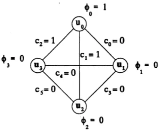
Here there is 1 faulty unit (U,,) and 1 erroneous com- parison result (co) as in figure 2.

The objective of testing a system is to find out whether a failure exists in the system at the time of the test, and then

to locate any failed unit(s). After the fault location process is completed, some level of repair or reconfiguration must be initiated.

+ = o

₃

4 =

1

' 0 1

@

- 0

Figure 2. Possible Comparison Outcome with 1 Faulty Unit

2.3 Likelihood Table

The Ciaj can be combined into a likelihood table (LT) listing all the values of Pr {

Ci

laj}

; LT is a probabilistic com- parison table and can be computed prior to operation of the system, however its storage size is O(2"- U "), eg, table 1 for the system in figure 1.

Chang [6] developed an analytic method to avoid the need to store this enormous amount of data. The method requires

O(m)

time to retrieve a data item or O(1og m) time when prestored reference data are used. The number of data items retrieved at test time is small and has an absolute upper bound of 7. Section 6 provides an illustration.

3. ASSIGNMENT OF MULTIPLE TEST SETS Tests T ( k ) are repeated 7 times, thereby attempting to

achieve pseudo-exhaustive testing [27], with variation of the individual tasks ti within a class of test tasks, both to improve test coverage, since the test might not be complete, and account for random effects in the test environment as discussed in the Introduction.

The 7 comparison results are conditionally s-independent,

ie,

7

pr {

c

( 1.. . 7 )

I$}

=

n

Pr{c(s)14jj.),

s = l

Pr

{ C(')

I aj}

can be obtained from the probabilistic comparison table for j = 0, 1,

...,

2"-1. Consequently, the posterior distribution can be evaluated by Bayes theorem:

460 IEEE TRANSACHONS ON RELIABILITY, VOL. 43, NO. 3, 1994 SEPTEMBER

*O

m oo01 *I

TABLE 1

Likelihood Table of Pr{Cjl*j}

Ip=0.95, q=0.90, r=0.75; the Pr{C,Jaj} values are multiplied by lo4]

0010 0011 0100 0101 0110 0111 loo0 1001 1010 1011

*2 *3 *4 *5 * 6 *7 *E *9 *IO *I1 *I2

1100 ~ C,=CXlOOOO c, = m 1 q = m 1 0 C4=oo0100 C5=oo0l0l C,=oo0110 c8=001000 ~ = O o l O o l c,o =001010

c,

,

=001011 c,2=001100 C3=oooOll C7 = oo01 1 1 CI3=OOllOl Cl4 =00lllO Cl5 = 001 11 1 C,6 = 0 1 m c,,=o1oo01 c,8=010010

c,

=010100

,

,

=010101 ~ = O l O l 1 0 q3=010111 q , = O l l O o O C,=Oll001 q 6 = 0 1 1010 q7=0i1011

q8

= 01 1 100

c,

=011101 C,=Olll10

c3,

=oil111

c33=

loo001 c, = loo010 c35 = loo01 1 c, = 100100 c37= 100101

c3,

= 1001 10 C,=lOloo0 c,, = 101001 c,, = 101010 c43 = 10101 1 C,=lOll00

c,=

1011 10 c,, = 101 11 1 c, = 1 1 m c49 = 1 loo01 C,=ll00lO c,, = 110100

css

= 110101 C,=llOllO c5s = 1101 11 c , = 1 1 lo00 cS8= 11 1010 C,=llll00 c,, = 111 101 c,, = 11 11 10

c,,

= 11 11 11 CI9=OlOOl 1 C32 = 1OOOOO c39 = 100111 C45 = 101 101 C5, = 1 1001 1 c57 = 1 1 1001 c59 = 11 101 1 7351 387 387 20 387 20 20 1 387 20 20 1 20 1 1 0 387 20 20 1 20 1 1 0 20 1 1 0 1 0 0 0 387 20 20 1 20 1 1 0 20 1 1 0 1 0 0 0 20 1 1 0 1 0 0 0 1 0 0 0 0 0 0 0 9 77 77 694 77 694 694 6250 0 4 4 37 4 37 37 329 0 4 4 37 4 37 37 329 0 0 0 2 0 2 2 17 0 4 4 37 4 37 37 329 0 0 0 2 0 2 2 17 0 0 0 2 0 2 2 17 0 0 0 0 0 0 0 1 9 77 0 4 0 4 0 0 77 694 4 37 4 37 0 2 77 694 4 37 4 37 0 2 694 6250 37 329 37 329 2 17 0 4 0 0 0 0 0 0 4 37 0 2 0 2 0 0 4 37 0 2 0 2 0 0 37 329 2 17 2 17 0 1 0 1 2 6 2 6 19 58 2 6 19 58 19 58 173 519 2 6 19 58 19 58 173 5 19 19 58 173 519 173 519 1558 4675 0 0 0 0 0 0 1 3 0 0 1 3 1 3 9 27 0 0 1 3 1 3 9 27 1 3 9 27 9 27 82 246 9 0 77 4 0 0 4 0 77 4 694 37 4 0 37 2 0 0 4 0 0 0 0 0 4 0 37 2 0 0 2 0 77 4 694 37 4 0 37 2 694 37 6250 329 37 2 329 17 4 0 37 2 0 0 2 0 37 2 329 17 2 0 17 1 0 2 1 6 2 19 6 58 2 19 6 58 19 173 58 519 0 0 0 0 0 1 0 3 0 1 0 3 1 9 3 27 2 19 6 58 19 173 58 519 19 173 58 519 173 1558 5 19 4675 0 1 0 3 1 9 3 27 1 9 3 27 9 82 27 246 0 2 2 19 0 0 0 1 1 6 6 58 0 0 0 3 2 19 19 173 0 1 1 9 6 58 58 5 19 0 3 3 27 2 19 19 173 0 1 1 9 6 58 58 519 0 3 3 27 19 173 173 1558 1 9 9 82 58 5 19 519 4675 3 27 27 246 0 0 0 1 1 4 4 13 0 1 1 4 4 13 13 38 1 4 4 13 13 38 38 114 4 13 13 38 38 114 114 342 1 4 4 13 13 38 38 114 4 13 13 38 38 114 114 342 13 38 38 114 114 342 342 1025 38 114 114 342 342 1025 1025 3075 9 0 0 0 77 4 4 0 0 0 0 0 4 0 0 0 77 4 4 0 694 37 37 2 4 0 0 0 37 2 2 0 77 4 4 0 694 37 37 2 4 0 0 0 37 2 2 0 694 31 37 2 6250 329 329 17 37 2 2 0 329 17 17 1 0 2 2 19 1 6 6 58 0 0 0 1 0 0 0 3 2 19 19 173 6 58 58 519 0 1 1 9 0 3 3 27 2 19 19 173 6 58 58 519 0 1 1 9 0 3 3 27 19 173 173 1558 58 519 519 4675 1 9 9 82 3 27 27 246 0 2 0 0 2 19 0 1 2 19 0 1 19 173 1 9 1 6 0 0 6 58 0 3 6 58 0 3 58 5 19 3 27 2 19 0 1 19 173 1 9 19 173 1 9 173 1558 9 82 6 58 0 3 58 519 3 27 58 5 19 3 27 519 4675 27 246 0 0 1 4 0 1 4 13 1 4 13 38 4 13 38 114 0 1 4 13 1 4 13 38 4 13 38 114 13 38 114 342 1 4 13 4 13 38 114 13 38 114 342 38 114 342 1025 4 13 38 114 13 38 114 342 38 114 342 1025 114 342 1025 3w5 38 0 0 2 0 2 0 19 1 2 0 19 1 19 1 173 9 2 0 19 1 19 1 173 9 19 1 173 9 173 9 1558 82 1 0 6 0 6 0 58 3 6 0 58 3 58 3 519 27 6 0 58 3 58 3 519 27 58 3 519 27 519 27 4675 246 *I3 1101 0 1 0 4 0 4 1 13 1 13 4 38 4 38 13 114 1 13 4 38 . 4 38 13 114 13 114 38 342 38 342 114 1025 0 4 1 13 1 13 4 38 4 38 13 114 13 114 38 342 4 38 13 114 13 114 38 342 38 342 114 1025 114 1025 342 3075

-

*I4 1110 0 1 1 13 1 13 13 114 0 4 4 38 4 38 38 342 0 4 4 38 4 38 38 342 1 13 13 114 13 114 114 1025 0 4 4 38 4 38 38 342 1 13 13 114 13 114 114 1025 1 13 13 114 13 114 114 1025 4 38 38 342 38 342 342 3075

-

1111 *i5 2 7 7 22 7 22 22 66 7 22 22 66 22 66 66 198 7 22 22 66 22 66 66 198 22 66 66 198 66 198 198 593 7 22 22 66 22 66 66 198 22 66 66 198 66 198 198 593 22 66 66 198 66 198 198 593 66 198 198 593 198 593 593 1780

CHANG ET AL: BAY= ANALYSIS OF FAULT LOCATION ON DISTRIBUTED SYSTEMS 461

TABLE 2

Simplified Bitwise Likelihood Table of Pr{Cll&] [Based on table 1. Pr{+,=O} =0.8, Pr{&=l} = 1 -0.8=0.2, for all k. The Pr{C,laj} values are multiplied by

lo4.

See table 1

for the bit-patterns for each C,.] (3)

I

4jI.

fi {+j} p r { c ( l ... 7 ) P ~ { $ ~ I c ( ' . . . ~ ) } = 2"-1

c

pr{c(l-.T)

I4jl

*fi{+i) i=o

j = 0, 1,

...)

2"-1. &)=o & ) = I g , = o +1=1 &=O 42=1 6 3 = 0 d3=1 As a rationale for the prior distribution on the parameter

of interest,

+ € e ,

we assume, as others have done, that ip

$J,,-~

...

$,, is i.i.d. with an exponential distribution [19,28,29,34,37,38]. The choice of the prior probability

Pr{@}

does not affect the discussion in section 4. Hence the procedure is robust with respect to the choice of the prior distribution.

4. BAYES ANALYSIS OF FAULT LOCATION 4.1 Background

In general, there are two ways to locate faults using Bayes analysis.

1. As in classical inference methods that mostly deal with the posterior distribution, choose either point estimation or set estimation to locate a fault [6,8-131.

2. Use a loss function and turn the problem into one from decision theory.

We use #2, the Bayes decision-theoretic approach, which enables us to estimate the fault status of each unit by point estimation with the choice of a reasonable loss function [2]. Distance is a reasonable measure for all misdiagnosed results. The loss function is computed bitwise from the global fault pat- tern. We use this loss function because it is computationally efficient and its center mean & mode are the same.

To assist the Bayes analysis, it is necessary to transform the likelihood table, Pr {

Cil

ipj}, to a bitwise version of the likelihood table, Pr { Ci

1

&}. As shown in table 2, the number of columns (which was 2" in table 1) has become simply 2n. We extend the expressions from previous sections and consider the case

4k

= 6, where 6 = 0 or 1 , to obtain:

(4) The marginal probabilities Pr{CiJ&},

k

=

0,

...,

n-1 in table 2 are generated from the conditional probability distribu- tion in table 1. Hence the column sums of the table are 1, but this is not true of the row sums

-

as anticipated. Table 2 is generated using (4) and was validated by two different programs written separately in the C & Matlab languages. The shape of the distribution in each column is similar to that in table 1 but the rate at which the values decrease is slower

than

in table 1.

This

observation is reasonable since the bitwise conditional distribution in table 2 compresses all possible fault conditions of S given the fault status,

4k=6,

of a single unit. Although

this bitwise distribution has a less pronounced shape than the CO CI c2 c 3 c 4 c 5 c 7 C8 c 9 CIO Cl 1 c12 CIS C18 c 1 9 c20 C2I c22 cz4 c25 c6 c13 cl, cl, c17 c23 C26 c27 c2S c29 c3 1 c32 c30 c 3 3 c34 c 3 5 c 3 7 C38 c 3 9 ca c 4 3 c44 c 4 5 c 4 6 c 4 7 C48 c 4 9 cso C5l c52 c 5 3 c 5 4 c55 c 5 7 C58 c 5 9 CLW c36 c41 c42 c56 c61 c62 cb3 3767 208 208 12 208 12 12 2 218 101 101 12 13 11 11 4 218 101 13 11 101 12 11 4 101 804 17 60 17 60 52 15 218 13 101 11 101 11 12 4 101 17 804 60 17 52 60 15 101 17 17 52 804 60 60 15 20 76 76 159 76 159 159 49 5 40 40 360 40 360 360 3224 1 6 6 37 8 51 51 312 1 6 8 51 6 37 51 312 3 13 26 86 26 86 214 674 1 8 6 51 6 51 37 312 3 26 13 86 26 214 86 674 3 26 26 214 13 86 86 674 5 23 23 99 23 99 99 404 3767 208 218 101 218 101 101 804 208 12 101 12 13 11 17 60 208 12 13 11 101 12 17 60 12 2 11 4 11 4 52 15 218 13 101 17 101 17 20 76 101 11 804 60 17 52 76 159 101 11 17 52 804 60 76 159 12 4 60 15 60 15 159 49 5 40 1 6 1 6 3 13 40 360 6 37 8 51 26 86 40 360 8 51 6 37 26 86 360 3224 51 3 12 51 312 214 674 1 8 3 26 3 26 5 23 6 51 13 86 26 214 23 99 6 51 26 214 13 86 23 99 37 312 86 674 86 674 99 404 3767 218 208 101 218 101 101 804 208 101 12 12 13 17 11 60 218 101 13 17 101 20 17 76 101 804 11 60 17 76 52 159 208 13 12 11 101 17 12 60 12 11 2 4 11 52 4 15 101 17 11 52 804 76 60 159 12 60 4 15 60 159 15 49 5 1 40 6 1 3 6 13 40 6 360 37 8 26 51 86 1 3 8 26 3 5 26 23 6 13 51 86 26 23 214 99 40 8 360 51 6 26 37 86 360 51 3224 312 51 214 312 674 6 26 51 214 13 23 86 99 37 86 312 674 86 99 674 404 3767 218 218 101 208 101 101 804 218 101 101 20 13 17 17 76 208 101 13 17 12 12 11 60 101 804 17 76 11 60 52 159 208 13 101 17 12 11 12 60 101 17 804 76 11 52 60 159 12 11 11 52 2 4 4 15 12 60 60 159 4 15 15 49 5 1 1 3 40 6 6 13 1 3 3 5 8 26 26 23 40 6 8 26 360 37 51 86 6 13 26 23 51 86 214 99 40 8 6 26 360 51 37 86 6 26 13 23 51 214 86 99 360 51 51 214 3224 312 3 12 674 37 86 86 99 312 674 674 404

-

462 IEEE TRANSACTIONS ON RELIABILITY, VOL. 43, NO. 3, 1994 SEPTEMBER

global distribution in table 1, table 2 is far smaller. Together with the bitwise method in this section, the small size of the table appreciably reduces the complexity of the analysis. Besides that, P r { c i l & = o } f P r { C i l & = 1 } in general. Such an equality, rarely occurring in practice, would yield an in- conclusive test result and compromise the comparison steps in the diagnosis process (see step 3 of BWB in this section and remark 5.5).

4.2 Point Estimation

Use the obseryed comparison pattems to determine &ML

=

...

&

...

4o

E

e.

+m is the ‘generalized maximum likelihood estimate’ of

+,

viz, the largest mode of the posterior distribution

Pr{@

I

d’-”}

[2: p 1331;

this

maximum likelihood estimate is anticipated to be unique. It is O(2”) to examine all

E 8 to find the maximum of all the Pr{91 C(’-‘)} if all have to be examined. However, [8,10] gave a heuristic-based search algorithm to find

6m;

it has only O(n) worst case com-

plexity to locate the faults with a 1 -a s-confidence level [2: p 4141.

-

4.3 Set Estimation

It is possible to obtain the 1 -a highest posterior density (HPD) credible region for the r.v.

e,

given some s m a l l real number a. To calculate the HPD we consider all subsets

r’

c

8 such that Pr{r’

1

C(’-.’)} 1 1 -a. Among these subsets

r

’

we must find the one with the highest density of posterior probability, viz, the subset such that ~ ( r ’ ) = min(Pr{aj1

c(

1.. . r ) }:

The HPD for @ is the subset

I’

which maximizes ~(r’): E

r’)

is the largest.

The computation cost of finding all such

r

’ is exponential. An alternative is to find a set I” for which the

Pr{@ji)C(l-.r)}

for all @j E

r

’

are relatively large and use that

r

’

as a reasonable replacement for

r

.

since

&m

is the most likely system fault pattem, the other fault pattems

3

E 8 can be considered as

misdiagnosed. Hence the number of misdiagnosed units can be used as a measure of distance of any fault pattem from

&m.

Notation

d ( A , B ) distance between A & B

@ ‘exclusive OR’ operation, The

Pr{$jlC(1...7)}

decreases as d(@j,

we construct

r’

using only those +j closest to &ML. [6,8,10]. Hence

n-1

d(&,

3)

E I&-+j,kl, wthatd(&, @ j ) E {0,1,...,n} k=O

Furthermore, since

&

=

o

or I , and 4 j , k =

o

or 1, it follows that:

n-1 n-1

k=O k=O

n-1

k=O

The remaining step is to construct a l-a credible region for @ which we anticipate to approximate the HPD region. Although

Pr{+jlC(1-.7)]

does not necessarily decrease as

d(&,,

3)

increases, the fault pattem with fewer misdiag- nosed

links

should appear more freque?tly. Therefore we in- clude the that have the smallest d(@’ML, Gj) first. In this

manner, it is possible to find the minimu? h

E

(0, 1, 2,

.

..,

n} such that if

r

=

{aj

E 8 : 0 I d(iPML,

3)

I h} then Pr(I’(C(’-‘)} 2 1-a. Thus, the region is a l-a credible region for

a.

Since

I’

does not necessarily contain all E

8

that have higher posterior density than

3.

f

r,

I’ cannot be assumed to be the 1 - a HPD credible region for Cp. However, the computation of

I’

is more efficient.

4.4 Bayes Decision Theoretic Approach

We now

turn

to the decision theoretic approach to point estimation. A decision rule is a mapping from the test results

C ( l - . r ) to the fault pattems

3:

Given a particular test result, the rule decides on a particular fault pattem. The Bayes approach considers the true fault pattem which we denote by iP

=

...

t$k

. . . 40,

although it is unknown, of cuurse. We must then choose a reasonable loss function. In section 4.3, we claimed that distance is a reasonable measure of the amount of misdiagnosis in a pattem. Given the test result C(1-.7) suppose an arbitrary decision rule assigns the fault pattem

4

= &-I

.

.

.&.

.

.60

E

e.

Then consider the loss function: n-1 n - I

k=O k=O

n-1

k=O

The statistical importance of this function is that, since Cbk &

&

only take the values 0 & 1 , it has the same properties as the square-error loss and absoluteerror loss. Moreover, the loss function is computationally practical since it can be evaluated by the ‘exclusive OR’ operation which is efficient. This shortens the unit computation time.

Given a loss function, we have to consider the fact that CP is unknown and, in fact, every

aj

is possible and, given

C(l-.T), the probability of Q, being is exactly the posterior probability P r { 3

1

C(1,..7)}. We define a risk function p as the s-expected loss, given this probability distribution for

*:

CHANG ET AL: BAY= ANALYSIS OF FAULT LOCATION ON DISTRIBUTED SYSTEMS

In this equation the r.v. which is conditionally s-dependent on

~ ( 1 . . .r) is ip. The risk function can be expanded to explicit sums

as follows, but the sums here are over 2" elements:

* E 9

Now we can select the Bayes decision rule which makes

...

4;

...

4;

E 0, to be the correspond to ipi =

c(1 . . . T )

one that minimizes the risk function:

n - 1

k = O

The

full

derivation is given in [6,13]; and the r.v. which are conditionally sdependent on C(l...r) are 9 and its components

&.

Then =

+.*-1...r#$...40.

minimizes p(4$,

a)

iff

4;

minimizes p ( # ,

4)

for all

k =

0, 1, 2,

...,

n-1. Hence the complex global analysis of all the ih

E

0 is decomposed into a simple bitwise analysis. In other words, in order to compute the i p i assigned by the global Bayes decision rule, it is suffi- cient to find all bitwise assignments

4;

= 0 or 1

(k

= 0, 1,

2,

...,

n-1) that minimize:

463

replaced by the sum of two terms! However, it can be reduced further by using the fact that:

since

4:

&

&

are binary variables, we know that if

42=O,

then Hence:

4!@

4k

=

4k.

Therefore,

The decision process outlined above can be summarized as the following bitwise

(BWB)

version of the Bayes decision algorithm to perform fault location:

4.5 BWB for Fault Location

Choose the components

4;-

For each

k

= n-1,

...,

0:

1. If

r(&;

l }

>

r(rbk;

0}, then choose

4;

= 1. 2. If

I(&;

l}

<

r(&;

0}, then choose

4;

= 0.

3. Otherwise, the test is inconclusive.

If a set estimation is desired, the procedures developed in section 4.3 can be applied to ?btain a 1 -a credibility region for ip by substituting ip; for

&.

.+;.

.

.&

of 4$ as follows:

or equivalently minimize the numerator,

5 . REMARKS

The complexity of analysis, by using this methodology, has been reduced dramatically since sums with 2" terms are

7

5.1 Pr{C(l..,r)l&} = Pr{C(S)(r&} s = l

is computable, since Pr{C(')I&} can be obtained from the simplified bitwise likelihood table, eg, table 11. Furthermore, the size of this likelihood table is 2"-n-2 = n.2"+', which

~

464

is much smaller than 2m 2" = 2m+" of the full likelihood table such as table I. Also the data in the both tables can be com- puted prior to run-time.

5.2 The run-time complexity of BWB is 0 (n). This use of bitwise analysis dramatically surpasses previous results in the literature and is a very good result in theory & practice. From the theoretical point of view, it reduces the complexity of the Bayes analysis; this complexity is one of the main defi- ciencies of the Bayes approach. In practice, BWB outperforms other methods in the literature since it does not really require any assumptions. The only disadvantage is in the generation of the probabilistic comparison table. Again, this is a one time computation.

5.3 Since the loss function is square-error loss, the posterior mean E{4klC(1.-r)} is the Bayes rule [2: p 161, result 31. However, because

4;

is binary, it is reasonable to choose r#= 1 if E{4kIC(1...r)}

>

0.5 (the same decision rule as step 1). If the loss function were generalized to a weighted square-error loss, then the Bayes rule can also be obtained [2: p 161, result 41. However, that form of the Bayes rule is not as simple as the BWB. In addition, since the loss function is also the absolute error loss, the median of Pr{&l C('...')} also provides a Bayes rule [2: p 162, result 51. Again, since @ is binary, this is equivalent to the BWB. If the loss function is generalized to a linear loss, the decision rule can be obtained in a similar fashion [2: p 162, result 61. Thus, BWB is valid for a class of the usual loss functions.

5.4 BWB is consistent with one's intuition and has the im- portant property of positive Bayes decision rules, namely ad- missibility. This gives extra trust in our intuition.

5.5 If the inconclusive test result described in step 3 of

BWB were to occur, it could be resolved by upgrading the quali- ty of the test tasks ti or by increasing 7 , the number of tests.

The latter would be necessary if faults were intermittent. 5.6 BWB accommodates all possible faulty & fault-free systems under test, without any increase in complexity when the fault-free state is diagnosed, permitting the algorithm to be applied to monitor a system periodically. Further, BWB is able to distinguish truly faulty units from those which appear faulty due to the imperfect environment, thus eliminating unnecessary hardware replacement or reconfiguration before the system recovery process performs rollback to a fault-free state.

5.7 The comparison-based probabilistic model and the Bayes inference algorithm make BWB complete in the statistical sense, since the model together with the BWB can accommodate all possible random effects. It is practical because the computa- tions are simple binary operations, with linear complexity. The necessary data are directly observable during the testing process.

5.8 A visual simulation tool (ViSiT) [7] has been im- plemented in C f + to test the validity of BWB. Test results have demonstrated that the algorithm is both efficient & ac- curate. When testing the algorithms for the early phase of system operation, 98% of the tests gave exact fault coverage. For tests corresponding to the late phase of system operation, 85% of the tests gave exact fault coverage. In both cases, the remain-

ing tests diagnosed as faulty both the actual faulty units and some of the fault-free units. ViSiT also demonstrates that the excess

IEEE TRANSACHONS ON RELIABILITY, VOL. 43, NO. 3, 1994 SEPTEMBER

of fault-free units being misdiagnosed begins to show when the fraction of faulty units exceeds 50%.

6. EXAMPLE OF LOCATING SYSTEM FAULTS Figure 1 is a 4-unit system; figure 2 shows the possible comparison outcome with 1 faulty unit. Let 7= 10. The follow- ing comparison patterns are observed:

These patterns are sorted & counted as follows:

Patterns (sorted) CO Clo C34 Ca C42 C57

count 1 1 1 2 4 1

According to BWB, all we need to do is to sum Pr{C(1-.10)14k = l } . P r ( ~ , = l } from table 11 and compare it with the cor- responding sum of Pr{C('-lo)l+k=O} .Pr{4k=0}. Repeat the same step until all the bits are done: k = 0 to 3, in this case. This also implies the bitwise computations are carried out only on the relevant

4k

column. Let k=O and compute for

40=

1:

Similarly, for qjO=O:

pr {

c"

. ..IO) I&=O} -Pr{40=0} = 10-40*[3767*101 * 101

-

10l2

-8M4 *76]

-

(0.8).

Since P r { C ( l ~ - * o ) ~ ~ o = l } -Pr{+o=l) is obviously smaller than pr {

c"

. . .lo) ~ ~ o = O } ~ P r { ~ o = O } , we choose

4;=0.

In the next step, k is increment4 by 1 and the process repeats. We con- clude from the iterations of BWB that the fault pattern of the system is ip' = +;+@;+; = 0100 = ip4.

ACKNOWLEDGMENT

We are pleased to thank Professor Jiunn T. Hwang for his helpful discussions and suggestions.

REFERENCES

[l] F. Barsi, "Probabilistic syndrome decoding in self-diagnosable digital systems", Digital Processes, vol I, 1981, pp 33-46.

[2] J.O. Berger, Staiistical Decision lheory and Boyesian Analysis (2"d ed), 1985; Springer-Verlag.

CHANG ET A L BAYES ANALYSIS OF FAULT LOCATION ON DISTRIBUTED SYSTEMS 465

P. Berman, A. Pelc, “Distributed probabilistic fault diagnosis for multiprocessor systems”, Proc. 20th Symp. Fault-Tolerant Computing,

D.M. Blough et ai, “Fault diagnosis for sparsely interconnected multiprocessor systems”, Proc. 19” Symp. Fault-Tolerant Computing, M. Blount, “Probabilistic treatment of diagnosis in digital systems”, Proc.

Th Symp. Fault-Tolerant Compwing, 1917, pp 72-77.

Y.L.C. Chang, “Characterization and analysis of the random nature of fault location”, PhD Dissertation, 1991 Dec; State University of New York at Binghamton.

Chang, Hsu, Hsu, Lam, Lander, Lau, Wu, “A visual simulation tool for design for diagnosability of dependable systems”, Proc. Int’l Conj:

Reliability & Quality in Design, 1994 Mar, pp 164-168.

Y.L.C. Chang, L. Lander, ”Classical inference methods for fault loca- tion in homogeneous systems”, Proc. IASTED Int ’1 Con$ Reliability. Quality Control, and Risk Assessment, 1992 Nov, pp 57-61.

Y.L.C. Chang, L. Lander, “Management of testing policies for fault location of failures dependent upon operation-time in multiprocessor systems”, Proc. IEEE 3rd Int’l Workshop on Responsive Computer

Systems, 1993, pp 166-172.

Y.L.C. Chang, L. Lander, “An inference design for fault location in real-time control systems”, J. Systems & sofrware (special issue on Fault

Tolerance in Real-Time Systems), vol 25, 1994 Apr, pp 3-21. Y.L.C. Chang, L. Lander, H. Lu, M. Wells, “Bayesian analysis for fault location in homogeneous distributed systems”, Proc. IEEE 12“ Symp. Reliable Distributed Systems, 1993, pp 44-53.

Y.L.C. Chang, L. Lander, H. Lu, M. Wells, “Bayesian inference for fault diagnosis in real-time distributed systems”, Proc. IEEE 2* Asian Test Symp. (ATs’93), 1993, pp 333-338.

Y.L.C. Chang, L. Lander, H. Lu, M. Wells, “The theory and applica- tion of Bayesian inference in system-level fault location”, Technical Report No. CS-TR-93-10, 1993 Aug; Dept. of Computer Science, SUNY-Binghamton.

K.Y. Chwa, S.L. Hakimi, ‘‘Schemes for fault tolerant computing: A com- parison of modularly redundant and tdiagnosable systems”, Informa-

tion and Control, vol 49, 1981 Jun, pp 212-238.

A.T. Dahbura, K.K. Sabnani, L.L. King, “The comparison approach to multiprocessor fault diagnosis”, IEEE Trans. Computers, vol C-36, 1987 Mar, pp 373-371.

D. Fussell, S. Rangarajan, “Probabilistic diagnosis of multiprocessor systems with arbitrary connectivity”, Proc. 1 9Ih Symp. Fault-Tolerant Computing, 1989, pp 560-565.

R. Gupta, I.V. Ramakrishnan, “System-level fault diagnosis in mhcious environments”, Proc. 171h Symp. Fault-Tolerant Computing, 1987, pp

184- 189.

S.L. Hakimi, A.T. Amin, “Characterization of the connection assign- ment of diagnosable systems”, IEEE Trans. Computers, vol C-23, 1974 Jan, pp 8688.

P.K. Lala, Fault Tolerance and Testable Hardware Design, 1985; Prentice-Hall.

L. Lander, Y.L.C. Chang, “Generation and analysis of probabilistic diagnostic information in homogeneous systems”, Proc. IASTED Int ’I Conf: Reliability, Quality Control and Risk Assessment, 1993, pp S. Lee, K.G. Shin, ‘‘Optimal multiple syndrome probabilistic diagnosis",

Proc. 20‘h Symp. Fault-Tolerant Computing, 1990, pp 324-331.

T. H. Lin, K. G. Shin, “Location of a faulty module in a computing system”, IEEE Trans. Computers, vol 39, 1990 Feb, pp 182-194. J. Maeng, M. Malek, “A comparison connection assignment for self- diagnosis of multipmssor systems”, Proc. I l l h Symp. Fault-Tolerant Computing, 1981, pp 173-175.

S. Maheshwari, S. Hakimi, “On models for diagnosable systems and probabilistic fault diagnosis”, IEEE Trans. Computers, vol C-25, 1976 M. Malek, “A comparison connection assignment for diagnosis of multiprocessor systems”, Proc. IO’h Symp. Fault-Tolerant Computing,

1990, pp 340-346.

1989, pp 62-69.

155-158.

Mar, pp 228-236.

1980, pp 31-36.

S. Mallela, G.M. Masson, “Diagnosable systems for intermittent faults”,

IEEE Trans. Computers, vol C-21, 1978 Jun, pp 560-566.

E.J. McCluskey, “Verification testing - A pseudo-exhaustive test techni- que”, IEEE Trans. Computers, vol c-33, 1984 Jun, pp 541-546. Y.W. Ng, “Reliability modeling and analysis for fault-tolerant com- puters”, PhD Dissertation, 1976; Dept. of Computer Science, UCLA.

D.K. Pradhan (Ed), Fault-Tolerant Computing: lheory and Techniques,

1986, chapter 8, vol II; Prentice-Hall.

F.P. Preparata, G. Metze, R.T. Chien, “On the connection assignment problem of diagnosable systems”, IEEE Trans. computers, vol EC-16,

1967 Dec. pp 848-854.

J. Russell, C.R. Kime, “System fault diagnosis: Closure and diagnosabili- ty with repair”, IEEE Trans. Computers, vol C-24, 1975 Nov, pp J. Russell, C.R. Kime, “System fault diagnosis: Masking, exposure, and diagnosability without repair”, IEEE Trans. Computers, vol C-24, 1975 A. Sengupta, A.T. Dahbura, “On selfdiagnosable multiprocessor 1078-1088.

Dec, pp 1155-1161.

systems: Diagnosis by the comparison approach”, Proc. 19Ih Symp.

Fault-Tolerant Computing, 1989, pp 54-61.

[34] D.P. Siewiorek, R.S. Swan, lke lheory and Practice of Reliable System

Design, 1982; Digital Press.

[35] L. Simoncini, A.D. Friedman, “Incomplete fault coverage in modular multiprocessor systems”, Proc. ACM Annual ConJ 1978, pp 210-216. [36] J.E. Smith, ‘‘Universal system diagnosis algorithms”, IEEE Trans. Com-

puters, vol C-28, 1979 May, pp 374-378.

[37] G. Sullivan, “System-level fault diagnosability in probabilistic and weighted models”, Proc. I Th Symp. Fault-Tolerant Computing, 1987,

[38] K.S. Trivedi, Probability and Starisrics with Reliability, Queuing, and-

Computer Science Applications, 1982; Prentice-Hall.

pp 190-195.

AUTHORS

Dr. Yu Lo Cyrus Chang; Dept. of Computer Science and Electrical Eng’g; The University of Tennessee; Chattanooga, Tennessee 37403-2598 USA. Yu Lo C. Chang (M’92) received his BS in Electrical Engineering from the National Taipei Institute of Technology and his MS & PhD in Computer Science from the State University of New York at Binghamton. He is an Assistant Professor in the Dept. of Computer Science and Electrical Engineering at the University of Tennessee at Chattanooga. His research interests include fault-tolerant computing, fuzzy systems, hard real-time systems, reliable parallel and distributed processing, statistical decision theory, VLSI testing, and visual synthesis tools. He is a member of IEEE Computer and Reliability Societies.

Dr. Leslie C. Lander; Dept. of Computer Science; State University of New York; Binghamton, New York 13902-6000 USA.

Leslie Lander (A’86) has a BA in Mathematics from Cambridge and a PhD in Mathematics from Liverpool. He taught in Brazil, Great Britain, Germany, Peru, and Venezuela before moving to Binghamton in 1984, where he is an Associate Professor in Computer Science. His interests include formal aspects software engineering, programming languages and system-level fault diagnosis. He is an Associate Member of IEEE and a Member of ACM. Dr. Homg-Shing Lu; Inst. of Statistics; National Chiao Tung Univ; Hsinchu

Horng-Shing Lu received his MS (1990) and PhD (1994) in Statistics at Comell University and BS (1986) in Electric Engineering at National Taiwan University. He is an Associate Professor in the Institute of Statistics at the National Chiao Tung University. He has authored papers in statistical computing methods, reliability, and nonparametric function estimation. He is a member

of the American s?ati&A Association and the Instilute of Mdlanab ‘cal statistics.

(Continued on page 469)

PORAT ET A L ESTIMATION OF PR(X > Y) OR PR(X <= Y) 469

Reliability obeys model I

n = 5

py = 50 pounds, Dy = 0.1, D, = 0.05.

An average of 1 units (for n = 5 ) fails at the severe test condi- tions. Thus, at the 95% s-confidence level, RL,s = /30.0~(4,2)

= 0.342. 4

R ~ , ~ = o . 9 9 9 , ’ 7 = 5 %

The result is:

A = 0.34216, B = -0.97613,

6

= 1.40.

The test level is therefore S = 5 0 . 1 . 4 = 70 pounds. of the reliability at the test level is:

During the test, 2 out of the 5 units failed. The 95 % LCB

working conditions based on poor reliability demonstrated at the test level.

REFERENCES

J. Hahn, S. Shapiro, Statistical Models in Engineering, 1967, pp 72-74;

John Wiley & Sons.

E. Parzen, Modem Probability and Its Applications, 1960, pp 237-238;

John Wiley & Sons.

G.W. Snedmr, W.C. Cochran, Sraristical Methoh, 1980, p 41; TheIowa State University Press.

N.R. Mann, R.E. Schafer, N.D. Singpurwda, Methoh for Statistical Analysis of Reliability and Life m a , 1974, pp 173-174, 289-293; John Wiley & Sons.

F. Clifton, “Strength variability in structural materials”, R&M -3654, 1971; Ministry of Aviation Supply, Aeronautid Research Council, Lon- don, Her Majesty’s Stationary Office.

E.B. Haugen, Probabilistic Mechanical Design, 1980, John Wiley & Sons. A. Mosleh, G. Apostolakis, Models for the Use of Expert Opinion in Low Probability, High Consequence Risk Analysis (R.A. Waller & V.T. Covello, Eds), 1981, pp 107-124; Plenum Press.

AUTHORS

px,L= 67 pounds

RL,N = 0.9977

<

0.999 (the requirement).

5 . PRACTICAL APPLICATIONS

The procedure is based on testing a few units at a severe level, rather than testing many units under working conditions. Typical situations are 4

-

5 units without failure in 20%

-

30% amplifidattenuated test levels rather than 200

-

300 units without failure under nominal working conditions.

While implementing the procedure, its underlying assump- tions should be thoroughly examined & tested to assess their validity in the given problem. The selected test level should not be too far from the working conditions, to prevent a change

in the failure mechanism. We recommend a “success-oriented approach” during the selection of the test level so that mainly successes are anticipated. Even though it is not a mathematical restriction, it is not desirable to deduce high reliability at the

Ze’ev Porat; RAFAEL (22); POBox 2250; Haifa 31021, ISRAEL. Internet (e-mail): mo&@actcom.co.il

Z. Porat has been employed by RAFAEL as a senior reliability engineer since 1976. He spent the years 1986-1988 at Bell Communications Research, Red Bank as a reliability analyst. He obtained his BSc (1976) in Industrial & Management Engineering from the Technion - Israel Institute of Technology, Haifa.

Meir Haim; RAFAEL (22); POBox 2250; Haifa 31021, ISRAEL. M. Haim has been a reliability analyst at RAFAEL for the past 15 years and has analyzed reliability & safety of complex systems. During this period he spent a year of dealing with reliability research at the University of Califor- nia, Los Angeles. M. Haim obtained his MSc (1976) in Operation Research from the Technion

-

Israel Institute of Technology, Haifa.

Yaffa Markiewicz; RAFAEL (46); POBox 2250; Haifa 31021, ISRAEL. Y. Markiewicz has been an operations research and reliability analyst

in RAFAEL since 1968. She obtained her MSc (1974) in Statistics from Stan-

ford University.

Manuscript received 1993 April 15.

IEEE Log Number 92-12071

Bayes Analysis

for Fault Location in Distributed Systems

( Continued from page 465 )

Dr. Martin T. Wells; Statistics Center and Dept. of E&S Statistics; Cornell University; Ithaca, New York 14853-3901 USA.

Martin T. Wellsis an Associate Professor of Statistics at Cornell Univer- sity. He received his PhD (1987) in Mathematics at the University of Califor-

and reliability. He is a member of the American Statistical Association and the Institute of Mathematical Statistics.

Manuscript received 1993 November 2‘