BUDGET MANAGEMENT OF NETWORK CAPACITY PLANNING BY SEARCHING CONSTRAINED RANGE AND DOMINANT SET

(1)

IEEE JOURNAL ON SELECTED AREAS IN COMMUNICATIONS, VOL. 12, NO. 6, AUGUST 1994 1031

Budget Management

of Network Capacity Planning

by

Searching Constrained Range and

Dominant Set

Chyan Yang, Senior Member, IEEE, and Ruey-yih Lin

Abstract-A communication network’s reliability, survivabil-

ity, and interconnectivity are primarily based on the degree of interconnection between the existing nodes of the network. En- hancement of these characteristics can be obtained by adding direct communication links between nodes of the network. This process is generally subject to a budget constraint. From the service provider’s perspective, enhancing the interconnectivity of heterogeneous networks is part of operations evolution. However, the interconnectivity or link enhancement problem, for a given budget, is NP-complete. Decisions by considering multiple criteria improve previous work and may search only the constrained range. The constrained range is determined by a dominant set of multiple criteria. A review of pertinent pre- vious work, problem formulation, algorithm presentation, and discussion of improving the computation time with compromis- ing the optimality by using the multiple-criteria constrained range are also provided.

I. INTRODUCTION

ETWORK management is the process of controlling

N

a complex data network so as to maximize its effi- ciency and productivity [5], [6], [ 113. Most network management tools are to monitor and report the network status or statistic. For strategic planning, the observations from network engineers will naturally lead to network capacity planning. Network capacity planning is the most time- consuming task to plan the changes required to keep the corporate communication network effective as a strategic asset while maintaining acceptable expenses [ 111. In both the telephone and computer networks, the network capacity planning is inevitably related to interconnectivity or survivability. Network interconnectivity has been studied mainly for the purpose of establishing fault-tolerant net- works. As fault-tolerant network is a direct consequence of good network management functions such as fault management, configuration management, and performance management [5], [6], [ 1 11. Many researchers have studied network interconnectivity based on concepts in graph theory that relate to either spanning trees [7]-[9] or

Manuscript received June 1993; revised February, 1994. This work was supported in part by the National Science Council under Grant NSC82-

The authors are with the College of Management, National Chiao Tung IEEE Log Number 9401457.

0113-E-009-294-T.

University, Hsinchu, Taiwan, Republic of China.

cutsets [12]. The specific problem of each research may be different, but the corresponding optimal solution to that problem can be proven intractable. Realizing the diffi- culty of the problems, several researchers have proposed heuristic approaches for solving network survivability problems [7], [ 121, [ 141-[ 161. Even with heuristic solutions, these algorithms are still computation intensive. In this paper, we show further improvements to the optimality and computation times [14]-[ 161.

It is common that an existing network consisting of many nodes will contain some nodes that are directly connected with communication links, while some of them have to communicate indirectly through immediate nodes. Sometimes, it is desirable to add communication links between nodes of a communication network enhancing the network interconnectivity

,

survivability, or performance. For an existing network, it is important and interesting to ask the question: What is the optimal link enhancement for a given budget?

Suppose we have a table for all pairs of nodes which are not yet connected. For each pair of the nodes

(i,

j ),

we have the information about the costs (cV) of establishing a link between them. In addition, we know the value

p i j for the performance contribution when the link be-

tween the pair of nodes

(i,

j ) is established. In the following discussions, we call pV a proJit that may simplify our usage of subscripts (since both “cost” and “contribution” start with “c”). The value pV can be thought of as the contribution of the link connecting node

i

a n d j , either in interconnectivity or survivability measures [8], [9],

[ 121. In our daily telephone communications, cij mainly indicates the cabling costs if the switching centers are to remain unchanged. It could be the reconfiguring costs of affected switching centers, whether the switches are in end offices, toll centers, o r primary centers. As for the p V , it could be thought of as the reduced circuit switching time (delay) of successful connections or the increased circuit utilization time that contributes to the profit of telephone companies. Only complete calls contribute to profits. Without a successful connection, circuit-switching activ- ities may keep the end offices and intermediate toll centers busy, but collect no revenue. Worse yet, congestions in a network tend to propagate and may halt the entire network [lo].

(2)

1032 IEEE JOURNAL ON SELECTED AREAS IN COMMUNICATIONS, VOL. 12, NO. 6, AUGUST 1994

Now, the question can be stated as follows. Given an investment or budget in dollar amount

B,

what is the best strategy of networking link enhancement such that the overall network will have optimal interconnectivity? Managerial considerations usually give a budget figure so

that, practically, we are solving the link enhancement problem with the given total costs. The link enhancement problem is NP-complete, and is reducible to the O/l-knapsack problem which is a known NP-complete problem [3], [4]. The discussion can be found in [ 141, [ 151.

For a given table size n , if we try all possible combinations of the link selections to decide the optimal solu- tion, i.e., a complete enumeration, we may need O ( 2 ” ) computation time in the worst case. This is because we have two choices for each link: to connect or not to connect. Solving this problem with the dynamic program- ming technique is also possible, but still intractable, i.e.

,

it takes O(2“) time [lo]. To understand why the optimal solution is so expensive and intractable, we need only consider a problem of size n = 60. The value 260 is on the order of In a calendar year, we have fewer than 10’’ ns. Assuming we have a GHz “super” computer than can test one alternative in 1 ns, then we need one century

(1019/1017) to test all 260 combinations. Given a budget of

7000, Table I shows an example of an n = 20 problem that demands 2” iterations to obtain the optimal solution. We will use this example to explain various algorithms used in the following discussions. We choose n = 20 because it is small enough to produce optimal solutions for sufficient sets of testing cases, and it is large enough to show that the task of finding its optimal solution manually is nontrivial.

Generally speaking, we should find an algorithm that provides near-optimal solution and takes nonexponential time to compute [l], [3], [4]. In this paper, we present the algorithms and explain the performance of the algorithm. In the following discussions, we assume that each link selection is independent of the others, except that the total budget B gets reduced. This is a reasonable assumption since usually we select only a small set (from 1 to 6)

of links, and the assumption will simplify the algorithm to be presented. In reality, after each link selection, we have to update the pij for the entire network before the next selection takes place. However, the computation of pij is beyond the scope of this paper, and its computation time should not affect our results. Detailed justifications are given in the next section.

The rest of the paper is organized as follows. Section I1 reviews and explains the linear search algorithms and presents the ideas of constrained range and reduced candidate set. Section I11 reviews four examples chosen from

[ 141: these examples are the only types of hard problems

that can be found in [ 141, and will be used to demonstrate the improvement of the new algorithm. Section IV explains the concept of dominant set and applies the multiple criteria decision [2] on four examples in the previous work. Section V concludes this paper.

TABLE I

EXAMPLE OF 20 LINKS TO BE CONNECTED A N D THE CORRESPONDING PROFIT Link number Cost Profit

1 1833 4140 1754 3506 2 3 1246 3819 4 1529 2310 5 2034 3370 6 2568 5276 7 1508 3859 1608 4477 8 9 1691 3269 10 2112 3807 11 1840 3661 12 1960 3560 13 2184 4440 14 2549 2899 15 2254 3643 16 2289 4224 17 1883 4368 18 1682 1922 19 1711 3844 20 1578 3484

11. CONSTRAINED SET AND REDUCED CANDIDATE

SEARCHES BY USING LINEAR SEARCH

ALGORITHMS

A computer network can be thought of as a graph G ( V ,

E), where V represents the vertices (nodes) and E represents the edges (links) [l], [4]. Suppose we have a table consisting of tuples of the form

(i,

j , clJ, p,) where i and j are the node numbers in the network and clJ is the cost to establish the link between node i and node j ; the value

p!, is the contribution of this interconnectivity or link en-

hancement. We are trying to find a solution for a given investment B such that

C

cl, 5 B and

C

plJ is maximized. We can describe a generic linear search algorithm with the following steps.

1 ) Select (remove) a link from the set of candidate links;

add this link to the current network. 2) B + B - clJ.

3) Update the network profile, i.e., compute plJ for the 4) Stop if B

<

clJ for all links.

5) Go to step 1 ) .

As we have mentioned above, step 3) will not be included in subsequent discussions. Practical applications justify this assumption: we generally have candidate links far apart, and a local adjustment will not affect remote areas or links. For instance, an expansion of switching capacity in a local end office of a telephone system or a reconfigured router of a local area network will hardly be visible to remote sites. Additionally, it hardly increases multiple links in a local area in capacity planning. In case we cannot avoid including step 3) in allocating the budget, we then must resort to adding one link at a time followed by a corresponding revision on thepb’s. The problem then is reduced to a trivial single-link problem, and many of the computations would be the iterative updates of pb’s Other than the practical measurement of plJ suggested in the last section, p v can also be measured by a network’s topological factors: the link connectivity factor (LCF) and new network.

(3)

1033

YANG AND LIN: BUDGET MANAGEMENT OF NETWORK CAPACITY PLANNING

the node connectivity factor (NCF). A detailed discussion on the computations of LCF and NCF can be found in

[7]-[9]. Even when the assumption of excluding step 3)

is relaxed, all the algorithms presented in this paper are still applicable, except that each iteration works on a revised table. The relative merits among the algorithms remain unchanged.

A . Linear Search Algorithms

There are three variations of the one-way linear search algorithm, and they differ at step 1) in the ways they select a communication link. We first sort the table in nonde- creasing order on the value of crJ and extract the tuples with a value of clJ I B to form a feasible solution set

called FS. A traditional optimal solution for the knapsack problem can be done by adding a field of rIJ = plJ/clJ to each tuple and sorting the list in nonincreasing order of

r I / . We call this new list FS,, and it consists of tuples of

(z,j, c y , p l J , rlJ). Without loss of generality, we can assign one link number to each node pair ( i , j ) to be considered, i.e., Table I shows only the link numbers instead of node pairs. Thus, in subsequent discussion, the list FS, consists of tuples of ( k , ck, Pk, rk) where k denotes the link number. Note that the value of rk effectively measures the contri- bution per dollar amount. The solution is simply a selection of links from the linear search of the list FS, until B is exhausted or becomes insufficient. If divisibility is al- lowed, this linear search algorithm, based on rlJ, gives the optimal solution 141 for knapsack problems. However, this solution will not give the optimal solution in 011-knapsack or link enhancement problems.

From FS, we can create two sorted lists FS, and FS,. FS, is sorted by clJ in nondecreasing order, while FS, is sorted by plJ in nonincreasing order. FS, of Table I is an ordered set ( 3 , 7 , 4 , 20

-

* 14, 6 ) since link 3 has min-

imum cost whereas link 6 has maximum cost. Similar to the linear search we have just described above, we can perform a linear search of list FS, and select links one at a time until the budget is exhausted or becomes insufficient. Likewise, we can do a linear search of list FS, and obtain the selections. Since all three one-way linear search methods, based on FS,, FS,, or FS,, are not optimal, we can always construct examples that defeat them easily. Note that in subsequent discussions, the ratios in FS, have been scaled up ( lo3) into integers for readability.

Instead of one-way linear search methods described above, we may make decisions by observing the two lists jointly. For example, we may use FS, and FS, together to obtain the selections. We start the linear search separately on these two lists, one link at a time. We use the voting or counting scheme to select the link. Whenever we en- counter a link such that the link has been visited in FS, or

FS,, the counter associate with the link is incremented.

When any counter reaches a preset threshold value, e.g., 2 , this link is added to the network. The value B is up- dated by subtracting ck of the candidate link. We continue

the linear search until B is either exhausted or becomes insufficient. This counting method is called a voting algorithm since each link accumulates the votes from different lists until it gets enough votes. The preset threshold in a two-way linear search is set to 2 since each link can get a maximum vote of 2. If the threshold is set to 1, the two-way search algorithm reduces to a one-way search.

B. The Best of Linear Heuristic Algorithms

All the heuristic algorithms discussed above are greedy in nature in that each sorts the FS in a certain order and allocates the available budget accordingly. Since sorting can be done in O ( n log n) time, we can achieve our so-

lution in O ( n log n) time. However, from our study, none of them consistently outperforms the others. It is natural to select the best among them, i.e., we can find seven sets of solutions and pick the best one from them. In the ex- ample of Table I, Srp provides the best solution of P , = 16 844. Solutions such as S,., S,, S,, S,,, S,,, SrP, are then ignored. By doing this, we select the best solution from a group of heuristic algorithms and call it BGH (the Best of Group of Heuristic). Unfortunately, even with six heuristic algorithms to choose from one cannot guarantee the optimal solution. The optimal solution of Table I is Sopt

= (3, 6 , 7, 8 ) with Popt = 17 431.

C. Constrained Range and Reduced Candidate Set

Two major improvements can be made over the linear search algorithms explained above: constrained range (CR) and reduced candidate set (RCS). The first method is to constrain the solution search space in a feasible range which is determined by the available budget and the given costs of links. To constrain the range, the method does not compromise the optimality ; the method simply tight- ens the feasible space. The second method, however, does compromise in trading computation time for the possibility of losing optimality. The combined method of CR and RCS is called CRCS. The first step of CRCS is to form the RCS, that is, to consider only those links that are can- didates in various linear search algorithms. It is this step that compromises the optimality. The second step of CRCS is CR, that is, to restrict the number of links to be selected in a constrained range instead of the entire range of [0, n]. We now explain in more detail. An example with numerical value can be found in Example 1 of the next section.

Given a budget B and costs of candidate links ci, we may find the optimum solution within a constrained range, hence saving computational costs. Let Cmin and C,,, be the minimum and the maximum ci, respectively. Notice that with the given B , we can readily compute the con- straints: the upper limit UL = LBICminJ and the lower

limit LL defined as

LL =

rB/Cmaxl if FS,(n - 1 ) 5 r LL = LB/Cmax] if FS,(n - 1)

>

r

(4)

1034 IEEE JOURNAL ON SELECTED AREAS IN COMMUNICATIONS. VOL. 12. NO. 6, AUGUST 1994

where r = B

-

E 7 = n - l + l F S , ( i ) , 1 = LB/CmaxJ

,

and

L

J

and

r

1

are floor and ceiling, respectively. LL indicates the number of links we can increase when all of the budget is used for each link that requires C,,,,,.

In a practical sense, this is the minimum number of links we can add. The ceiling in the LL expression represents the possibility that the leftover of BIC,,, may be sufficient for yet another link. If this possibility is void, the floor option is chosen for conservative computation. UL, however, represents the number of links that we can increase when all of the budget is used for each link that requires

Cmin. UL is the maximum number of links we can add. The floor in the UL expression represents the impossibil- ity that the leftover of B/Cmi, can be used for any other link since no link costs less than Cmin. The LL and UL give us the range in which the optimum solution should lie: [LL, UL] instead of [0, n ] . In other words, the number

of links we can add with the given budget is in the constrained range [LL, U L ] . In practice, once we obtain the solution from linear algorithms, we can squeeze this constrained range further and greatly reduce the computation time. We explain the squeezing methods in Section 11-D. The philosophy behind the RCS is that if a link should be in the optimal solution set, this link must have a high probability of being selected by one of the linear search algorithms. In other words, if we want to improve the result from the linear search algorithms, all we need is to examine only those links that have been selected by the linear search. This method, the RCS, rejects links that may or may not be in the optimal solution set; therefore,

it may not reach the optimal solution. Hopefully, the gain in this heuristic is justified by both a shorter computation time and a higher probability of reaching optimality. Let the contribution to the best solution from a linear algorithm using CRCS be Plinear.

In the previous section, the optimum solution was cal- culated within the range of [0, n] with the computational costs of O(2"): just for each of the n = 27 case, we used 37 user hours (single user) of VAXl1/785. Thanks to the CR for optimal solutions and CRCS for heuristic solutions, it is now practical to test 3960 cases up to n = 31 and they are reported in [ 141.

D.

Squeezing the Constrained Range

With the solutions of linear search algorithms, we can squeeze the constrained range for both the RCS and exact optimal solution. The maximum number k that satisfies

E:=

I F S , ( i )

<

Pllnear may squeeze the LL further: LL +

max(LL, k

+

1 ) . In other words, if the best k choices of

F S , ( i ) cannot beat the Pllnearr then we are sure that LL should be no smaller than k . By a similar scenario, the maximum number k that satisfies

E:=

I F S , ( i )

s

B may

squeeze the UL further: UL = min (UL, k ) . In other words, if the best k choices of FS, ( i ) are very close to B such that no more links can be added, then we are sure that UL must be no greater than k .

Example 1 : This example uses numerical values to illustrate the above discussions, and it shows that the CRCS method can find the optimal solution without an exhaustive search. We can apply a one-way linear search to the problem of Table I. For example, using FS, alone, with a budget of 7000, we can select links (3, 7 , 4 , 20) and achieve the total profit of 13 472. We call this set of links S,, meaning the solution set based on FS, only. The total profit obtained is called P,. Similarly, we can verify the following solutions: Sp = (6, 8, 13) and P, = 14 193, S, = ( 3 , 7 , 8, 17) and P, = 16 523.

In the two-way search, based on FS, and FS,, we obtain the solution S,, = ( 3 , 7 , 8 , 20) and P,, = 15 639. Sim- ilarly, one can show that S,, = S,,. Other possible meth-

ods of a two-way linear search are (FS,, FS,) and (FS,, FS,). Likewise, the heuristics cannot provide the optimal solution to the link enhancement problems. We may ap- proximate the optimal solution by examining all three lists, i.e., (FS,, FS,, FS,), as well. Similar to the two-way search, in a three-way linear search, we set the threshold value to 2. For these methods, we obtain the solutions and the corresponding total profit: 1 ) S,, = S, = { 1 , 7 , 8, 17) and P, = 16 844; 2) S,, = S,, = ( 3 , 7 , 8 , 19) and

Ppc = 15 999; and 3) S,, = ( 3 , 7, 8, 17) and P,, =

16 523. All other versions of three-way linear search al-

gorithms achieve the same solution set as S,,,,.

In Table I, the Cmin = 1246, while C,,, = 2568. Using the definitions above,

I

= L7000/2586J = 2 and r =

7000 - 5117 = 1883, r

<

FSc(n -

I )

= FS,(18) =

2289; hence, LL = 2 and UL = 5. The constrained search

range is [2, 51. Considering all possible combinations, we need to try C(20, 2)

+

C(20, 3)

+

C(20, 4)

+

C(20, 5) = 21 679 choices. Since 2*' = 1 048 576 and with a constrained range in [2, 51, we need only 21 679/1 048 576

= 2.06% of the original exhaustive computation time.

This is a tremendous savings! A further squeeze may reduce both LL and UL to 4; therefore, only C(20, 4) =

4 845 iterations or 0.46% of the original computation time

is needed. Note again that the methods used to constrain the search range and to squeeze the range do not compromise the optimality.

Recall that the reduced candidate set (RCS) is the set of all links that have been considered in various linear search algorithms. Therefore, in this example, we have

RCS = U

Si

= S, U S, U S, U S,, U S,, U S,, U S,, U s p c U S c p U Srpc U Srcp U s c r p U s c p r U Spcr U s p r c

= (1, 3, 4 , 6 , 7 , 8, 13, 17, 19, 20). The reduced candidate set has ten links to be considered, as opposed to the original n = 20. Note that, while the reduction of the search space reduces the computation time, it may compromise the optimality. Let us consider the case without squeezing methods first. Recall that the constrained range is now [2, 51. Therefore, instead of 21 679 choices as discussed above, we not have only C(10, 2)

+

C(10, 3)

+

C(10, 4)

+

C(10, 5) = 627 choices. The RCS im-

proved over the pure constrained range method by per- forming only 627/21 679 = 2. 9% of the former compu-

(5)

YANG AND LIN: BUDGET MANAGEMENT OF NETWORK CAPACITY PLANNING I035

tation. Comparing this to the brute force, purely exhaustive optimum, solution, the combined CRCS takes only 627/1 048 576 = 0.06% of the former computation. Considering the squeezing methods, we can limit the computation within C(10, 4) iterations to find the optimal solution. When both the optimal solution and the CRCS use the squeezing methods, the CRCS method uses only

C(10, 4)/C(20, 4) = 21014845 = 4.33% computation

time of that used by the optimal solution method. CRCS finds the best solution set of (3, 6, 7, 8) without the exhaustive search since these four links are in the reduced

candidate set.

0

111. HARD PROBLEMS

There are 3960 cases have been tested, and typical hard problems have been analyzed in [ 141. What makes a problem hard? A majority of the cases where the CRCS algorithm cannot find the optimal solution are due to insufficient resources: a linear search does not go far enough, and is forced to make premature decisions since B is al- ready exhausted. Examples 2 and 3 illustrate cases where CRCS cannot reach optimality [ 141.

Fortunately, an insufficient budget implies a narrow constrained range of the search space; hence, we do not need the RCS heuristic; we can simply apply the CR method alone and guarantee optimality. For a small constrained range, 2 or 3 in our cases, a polynomial time computation will reach the optimal solution. In general, the CRCS is still combinatorical, though the number of combinations is drastically reduced. The details of timing analysis can be found in [14]. The real difficult task, although there was only one occurrence in 3960 testing cases, comes from sufficient resources, but the distribu- tion of ci and p i prevents the CRCS from reaching opti- mality [14]. For this specific case, Example 4 shows the data set and analyzes the CRCS solution.

A. Examples

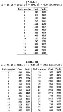
Example 2-Insuficient Resources: Table I1 shows one

typical case of insufficient resources: n = 15, B = 1500,

U : = 400, U: = 600, where U : and U: indicate the vari-

ance of c and p , respectively. Notice that the BGH solution comes from either FS,, or FS,, with the solution set

(2, 8) and contribution 7425. The reduced candidate set

of Table V is the set of all links that appeared in linear search algorithms: (1, 2, 8, 14, 15). Considering all

C ( 5 , 2) combinations, the CRCS reaches Plinear = 7425 with the solution set (2, 8 ) . The optimal solution, how- ever, is Pop, = 7581 with the solution set Sop, = ( 8 , 12). In this insufficient resource case, B = 1500, the BGH

reaches a decision early since the budget is exhausted in the first three iterations; the reduced candidate set is small since not enough links have been visited by the RCS method. Therefore, too small a candidate set excludes link 12 that should have been included, and selects links from

TABLE I1 n = 15, B = 1500, o f = 400, U ; = 600; EXAMPLE 2 Link number 1 2 3 4 5 6 7 8 9 10 11 12 13 14 15 Cost Profit 518 3219 689 3749 1133 2721 705 2607 1121 2940 1115 2674 1826 3600 643 3676 1997 3358 1100 2646 740 2576 832 3905 1097 2642 541 2936 1062 4016 TABLE 111 n = 2 8 , B = 2 8 0 0 , U : = 2 0 0 , U ; = 300; E X A M P L E S 3 Link number 1 2 3 4 5 6 7 8 9 10 11 12 13 14 cost 1049 1425 759 1073 827 1068 895 1550 769 1106 1065 1101 798 1036 - Profit 2973 3512 3288 2803 Link number 15 16 17 18 19 20 21 22 23 24 25 26 27 28 - Cost 925 965 821 1280 951 987 1042 1072 768 1010 758 758 905 849

-

Profit 3459 3484 3337 3438 2759 2766 281 1 2935 2975 2779 3102 3067 3443 2807

those appearing higher in the sorted lists: links 1 , 2 , and

Example 3-Znsuficient Resources: The data set of this

example is listed in Table 111. This is a hard case for the

BGH: the BGH algorithm gives ( 5 , 17, 27) as a solution for a contribution of 10 128, and CRCS improves it to

(5, 12, 17), giving 10 197 contribution. Using 10 197 as the lower bound of contribution, the optimal solution process revises the CRCS solution through steps of refinement: from 10 239 { 15, 17, 27), 10 264 { 16, 17, 27),

10 275 ( 5 , 16, 27), and then to the optimal solution

0

Example 4-Suficient Resources: Even with enough re-

sources, the CRCS method may still miss the optimal so-

lution. In one case of n = 23, listed in Table IV, the budget is large enough ( B = 1 1 500) to accommodate 12 links, which is more than half of the links. The starred links are in the optimal solution set. The solution from the CRCS, however, does not reach optimality

.

The best linear search algorithm is the S,, which gives the contribution of 37 768 (see Tables V and VI). The candidate set formed by linear search algorithms has 20 links to be considered, and RCS = ( 1 , 3, 4 , 5 , 6 , 7, 8,

9, 1 1 , 12, 13, 14, 15, 16, 17, 18, 19, 20, 21, 23); the reduced candidate set is quite large since 20 links out of a total of 23 links are qualified. The constrained range can be obtained as LL = BIC,,, = 1 1 500/1498 = 7 and UL

8.

0

(6)

IEEE JOURNAL ON

I036 SELECTED AREAS I N COMMUNICATIONS, VOL. 12, NO. 6 , AUGUST 1994

TABLE IV

n = 23, B = 11 500, u f = 200, U ; = 180; EXAMPLE 4

Link number Coat Profit 1* 796 3191 2* 1225 2963 3 1066 2916 4* 847 3104 5* 1003 2947 6 1057 2902 7* 693 3314 8* 823 3074 9 1498 3107 10 1242 2824 11* 891 3140 12* 916 3271 13* 957 3132 14 787 2746 15* 1031 3304 16 1067 2870 17* 1082 3127 18* 1187 3295 19 1107 2900 20 964 2812 21 1012 2868 22 1196 2818 23 801 2762 TABLE V

Fs,., Fs,,,

Fs,

OF EXAMPLE 4; L I N K S WITH * A R E I N OPTIMAL SOLUTION Link Id F S , Link Id FS, Link Id F S ,

7* 693 7* 3314 7' 4781 14 787 15* 3304 I* 4008 1* 796 18* 3295 8* 3732 23 801 12* 3271 4* 3661 8* 823 1* 3191 12* 3571 4* 847 11' 3140 11* 3522 l l * 891 13' 3132 14 3487 12* 916 17* 3127 23 3444 13* 957 9 3107 13* 3270 20 964 4* 3104 15* 3204 5* 1003 8* 3074 5' 2936 21 1012 2" 2963 20 2914 15* 1031 5* 2947 17* 2888 6 1057 3 2916 21 2832 3 1066 6 2902 18' 2775 16 1067 19 2900 6 2744 17' 1082 16 2870 3 2734 19 1107 21 2868 16 2690 18' 1187 10 2824 19 2619 22 1196 22 2818 2* 2418 2* 1225 20 2812 22 2355 10 1242 23 2762 10 2273 9 1498 14 2746 9 2073 TABLE VI

SOLUTION SETS OF EXAMPLE 4 BY LINEAR SEARCH ALGORITHMS

Algorithm FSr FSP FSc FSrp FSrc FSpr FSpc FScr FScp FSrpc FSrcp FSprc FSpcr FScrp FScpr Solution Set 7 1 8 4 12 11 14 23 13 15 5 20 7 15 18 12 1 11 13 17 9 4 8 7 14 1 23 8 4 11 12 13 20 5 21 7 12 11 13 15 8 17 18 6 3 16 7 1 8 4 14 23 13 5 20 15 21 6 7 111 13 4 8 5 18 6 3 21 19 7 1 11 12 13 4 8 5 6 16 21 18 7 1 8 4 11 12 13 5 20 15 21 6 7 1 11 12 13 4 8 15 3 17 19 18 1 12 11 14 23 15 5 20 17 21 18 1 12 11 14 23 15 5 20 17 21 18 1 12 11 14 23 15 5 20 17 21 6 16 1 8 11 14 23 15 5 20 17 21 6 16 1 8 4 14 23 15 5 20 17 21 3 16 1 8 4 14 23 15 5 20 17 21 3 16 Cost Used 10509 10721 10490 10770 10771 11439 11249 10990 11396 10470 10470 11407 11314 11279 11279 Contribution 36797 35059 36361 34345 36156 36783 37108 37059 37768 33463 33463 35940 35743 35721 35721 TABLE VI1 REVISIONS OF RCS; EXAMPLE 4

Step i Solution Set S, Cost Used Contribution 1 SI = {7,1,11,12,13,4,8,15,3,17,19,18) 11396 37768 3 S3 = {18,17,15,13,12,11,8,7,6,5,4,1} 11283 37801 4 S, = {18,17,15,13,12,11,8,7,5,4,3,1) 11292 37815 2 S2 = {19,18,17,15,13,12,11,8,7,5,4,1) 11333 37799

We cannot solely blame the small value of 0; since there

are many cases of the same 0 ; that can be solved effi-

ciently. As hindsight, one may observe that the optimal solution can be obtained by replacing the minimum contribution link (9) by the best feasible link (2). Note that among links in FS, not in SI, only link 9 has a better contribution than link 2, but using link 9 to replace link 19 in Ccp violates the cost requirement, that is, it exceeds the given budget. Since the nature of the effect of blending the cost and contribution makes the problem hard, replacing the link with a minimum contribution in the current solution set by a link with a higher contribution does not guarantee an improved solution. For instance, in Example

3, Plinear = 10 197 when the solution set is (5, 12, 17}, and none of the these three links is in the optimal solution set (15, 16, 2 7 ) . It is difficult to say which link in the optimal solution set replaces link 12, although link 12 has the maximum contribution.

= B/Cmin = 11 500/693 = 16. A further squeeze of the range reduces both LL and UL to 12. Examining combinations of 12-out-of-20 from the RCS, we can improve the solution in the steps listed in Table VI1 by selecting links from the RCS starting from the BGH solution FS,

(Step 1) and form the best solution set of { 18, 17, 15, 13, 12, 11, 8, 7 , 5 , 4, 3 , l } . This best solution set achieves

Plinear = 37 815. Unfortunately, the exact optimal solu- tion set is (18, 17, 15, 13, 12, 11, 8 , 7 , 5, 4, 2, l} with a contribution of 37 862; this optimal solution set differs from the optimal solution set based on RCS only by one

link.

0

Why does the optimal solution set in Example

4

above include link 2 when link 2 does not appear in the RCS?

IV. IMPROVED CONSTRAINED RANGE BY DOMINANT

A refined constrained range can be constructed, and hence reduce the computation time without a compromise in optimality. The revised UL is to examine

S,

and count how many links are included. The UL's of the above examples of n = 20, 15, 28, 23 are 4, 2, 3 , and 12, respectively. The revised LL is the link count in S,. The LL's of the above examples are 3 , 1, 2, and 1 1, respectively. The revised UL's and LL's are listed in the second column of Table IX. The philosophy behind this refinement is the same as the previous work [ 141, except not using the ex- treme values of C,,, and Cmin to bound the search ranges. Instead, the exact costs are used and the constrained range is further reduced. Additionally, without compromising

(7)

YANG AND LIN: BUDGET MANAGEMENT OF NETWORK CAPACITY PLANNING 1037

the optimality, one may reduce the candidate set described as follows into two computation phases: dominant matrix construction and candidate set partition.

First, we need to construct a dominant matrix: an n x

n matrix such that an entry d, at row i and c o l u m n j in- dicates the dominant relationship between link i and link j . The entry d, = 1 means that link

i

dominates l i n k j . A link i dominates link j if and only if ci

<

cj and p i

>

pi.

Therefore, the count of nonzero entries in a row i means the number of links that the link i dominates. Let W I N ( i )

denote this count. Likewise, the count of nonzero entries in a c o l u m n j means the number of links the l i n k j has been dominated, and is denoted as L O S S ( j ) . The con- struction of the dominant matrix requires O ( n 2 ) time. If

W I N ( i ) 1 ( n - U L ) , then link i must be in the final so-

lution candidate set to preserve the optimality. Why? This is because the selection of UL links will include link

i

if it were to have UL links in the optimal solution. The ex- clusion of link

i

will leave any selected UL links to form a suboptimal solution. If the optimal solution has fewer links than UL, link i many possibly not be included in the optimal solution. On the other hand, if LOSS( j ) L UL,

t h e n j cannot be in the final solution set. When L O S S ( j ) 2 UL for a l i n k j , there must exist at least UL links that dominate j , and hence no reason to include the link j in the final solution.

Having done the selection process by examining the

WIN and LOSS of each link, we have partitioned the orig- inal n links into three sets: excluded links (ELS), selected links ( S L S ) , and candidate links ( C L S ) . Note that n =

I

ELS

I

+

(SLS

I

+

1

CLS

1.

The optimal solution would be reduced to the enumeration of C (

1

CLS

1,

k

-

1

SLS

1)

where

k

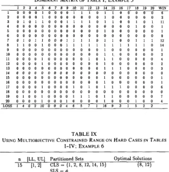
is a value in [LL, UL].

Example 5: The dominant matrix with its LOSS and

WIN of Table I is shown in Table VIII. Having counted the entries of LOSS and WIN, we know that CLS = { 1, 3, 4, 6, 13, 16, 17, 19, 20). Therefore, only C(9, 4) = 126 computations are needed without compromising the optimality. One can apply the same method in Tables II- IV. Table IX summarizes the results. Note that the hard- est case of n = 23 (Table IV) only requires C(15, 6 )

+

C(15, 7) or 11 435 tries to get the optimal solution. This multiple-criteria constrained range has only 15 links to choose from, and still guarantees optimality , unlike the larger RCS in Example 4 that has 20 links and has no guarantee of optimality

V. CONCLUSIONS

Available resources or budget are the most sensitive pa- rameters in the process of solving network link enhancement problems. A relatively small budget, that can afford only a few additional links, can utilize the exact optimal solution, which can be done in polynomial time. When the budget is sufficiently large to afford many additional links, the exact optimal solution can be too costly to compute. In this case, the use of the BGH method efficiently

TABLE VI11

DOMINANT MATRIX OF TABLE I; EXAMPLE 5

1 2 3 4 5 6 7 8 9 10 11 12 13 14 15 16 17 18 19 20 WIN 1 0 0 0 0 1 0 0 0 0 1 1 1 0 1 1 0 0 0 0 0 6 2 0 0 0 0 1 0 0 0 0 0 0 0 0 1 0 0 0 0 0 0 2 3 0 1 0 1 1 0 0 0 1 1 1 1 0 1 1 0 0 1 0 1 11 4 0 0 0 0 0 0 0 0 0 0 0 0 0 0 0 0 0 1 0 0 1 5 0 0 0 0 0 0 0 0 0 0 0 0 0 1 0 0 0 0 0 0 1 6 0 0 0 0 0 0 0 0 0 0 0 0 0 0 0 0 0 0 0 0 0 7 0 1 0 1 1 0 0 0 1 1 1 1 0 1 1 0 0 1 1 1 12 8 1 1 0 0 1 0 0 0 1 1 1 1 1 1 1 1 1 1 1 0 14 9 0 0 0 0 0 0 0 0 0 0 0 0 0 1 0 0 0 0 0 0 1 10 0 0 0 0 0 0 0 0 0 0 0 0 0 1 I. 0 0 0 0 0 2 11 0 0 0 0 1 0 0 0 0 0 0 1 0 1 1 0 0 0 0 0 4 12 0 0 0 0 1 0 0 0 0 0 0 0 0 1 0 0 0 0 0 0 2 13 0 0 0 0 0 0 0 0 0 0 0 0 0 1 1 1 0 0 0 0 3 14 0 0 0 0 0 0 0 0 0 0 0 0 0 0 0 0 0 0 0 0 0 15 0 0 0 0 0 0 0 0 0 0 0 0 0 1 0 0 0 0 0 0 1 16 0 0 0 0 0 0 0 0 0 0 0 0 0 1 0 0 0 0 0 0 1 17 0 0 0 0 1 0 0 0 0 1 0 1 0 1 1 1 0 0 0 0 6 18 0 0 0 0 0 0 0 0 0 0 0 0 0 0 0 0 0 0 0 0 0 19 0 1 0 0 1 0 0 0 0 1 1 1 0 1 1 0 0 0 0 0 7 20 0 0 0 0 1 0 0 0 1 0 0 0 0 1 0 0 0 1 0 0 4 L O S S 1 4 0 2 1 0 0 0 0 4 6 5 7 1 1 6 9 3 1 5 2 2 TABLE IX I-IV; EXAMPLE 6

U S I N G MULTIOBJECTIVE CONSTRAINED RANGE ON HARD CASES I N TABLES

~~ ~

n [LL, UL] Partitioned Sets Optimal Solutions

15 [l, 21 CLS = 11, 2, 8, 12, 14, 15) IS, 12) SLS = 4 CLS = { l , 3, 4, 6, 7, 8, 13 SLS = m 20 [3, 41 {3, 6, 7, 8) 16, 17, 19, 20) 23 [11, 121 CLS = (2, 3, 4, 5, 6, 8, 9, 11, 2, 4, 5, 7, 8, 11 12, 13, 15, 17, 18) 14, 15, 16, 17, 18, 20, 21, 23 } SLS = { l , 7, 11, 12, 13) 28 [2, 31 CLS = {3, 5, 10, 12, 13, 15, {15, 16, 27) 16, 17, 25, 26, 27) SLS = 4

provides a high probability of reaching optimality. The option of using the CRCS heuristic can further improve the probability of reaching optimality, and the extra computation time may be justified based on the span of the constrained range. Conflicting criteria may be combined into a single criterion for solving a complex problem; multiple-criteria constrained range searches illustrated in this paper are a good example that does not compromise the optimality and practically does not require extensive computational efforts.

ACKNOWLEDGMENT

This work was inspired mainly by previous work by M.

A. Schroeder, K. T . Newport, and G . M. Wittaker. The authors are also grateful to G . M. Wittaker for this en- couragement in providing many research points. Addi- tionally, the authors thank J. C. Su and M. K. Tsao, Tai- wan Long Distance Telecommunications Administration, for many helpful discussions. They are also indebted to the referees for their comments which gave the paper more practical value.

(8)

1038 IEEE JOURNAL ON SELECTED AREAS IN COMMUNICATIONS, VOL. 12, NO. 6, AUGUST 1994

REFERENCES

[ I ] A. V. Aho, J. E. Hopcroft, and J. D. Ullman, Design and Analysis

of Computer Algorithms.

[2] V. Chankong and Y. Y. Haimes, Multiobjective Decision Making: Theory and Methodology, Sys. Sci. and Eng. Ser. Vol. 8. Amster- dam: North-Holland, 1983.

[3] M. Garey and D. Johnson, Computers and Intractability: A Guide to the Theory of NP-Completeness. San Francisco, CA: Freeman,

1978.

141 E. Horowitz and S . Sahni, Fundamentals of Computer Algorithms.

Rockville, MD: Computer Science Press, 1978.

[ 5 ] F. Kauffels, Network Management: Problems, Standards and Strat- egies. Reading, MA: Addison-Wesley, 1992.

[6] A. Leinwand and K. Fang, Network Management: A Practical Per- spective. Reading, MA: Addison-Wesley, 1993.

[7] K. T. Newport, M. A. Schroeder, and G. M. Wittaker, “Techniques for evaluating the nodal survivability of large networks,” in Con$ Rec., 1990 IEEE Mil. Commun. Con$ , pp. 1108-1 113.

181 K. T. Newport and P. K. Varshney, “On the design of performance- constrained survivable networks,” in Con$ Rec. 1989 IEEE Mil. Commun. Conf., pp. 663-670.

191 M. A. Schroeder and K. T. Newport, “Enhanced network survivability through balanced resource criticality,” in Con$ Rec., 1989 IEEE Mil. Commun. Conf., pp. 682-687.

[IO] H. J . Siegel, Interconnection Networks f o r Large-Scale Parallel Pro- cessing. Lexington, MA: Lexington Books, 1985.

[ 1 I] K. Terplan, Communication Networks Management. Englewood Cliffs, NJ: Prentice-Hall, 1992.

[I21 G. M. Wittaker, M . A. Schroeder, and K. T. Newport, “A knowl- edge-based approach to the computation of network nodal survivability,” in Con$ Rec., 1990IEEEMil. Commun. Conf., pp. 1114-1119.

[I31 L. Wu and P. K. Varshney, “On survivability measures for military networks,” in Con$ Rec., 1990lEEEMil. Commun. Conf., pp. 1120-

1124.

[I41 C . Yang, “Link enhancement using constrained range and reduced candidate set searches,” Comput. Commun., vol. 15, pp. 573-580, Nov. 1992.

[I51 C. Yang and C. Kung, “Networking link enhancement with minimum costs,” in Con$ Rec., I990 IEEE Mil. Commun. Conf., pp.

Reading, MA: Addison-Wesley, 1974.

1125-1128.

[I61 C. Yang and L. Misirlioglu, “ A comparative study of networking link enhancement algorithms,” in Con$ Rec., 1992 IEEE Mil. Com-

mun. Conf., pp. 946-950.

Chyan Yang (S’86-M’87-SM’90) received the M S degree in information and computer science

from the Georgia Institute of Technology and the Ph.D. degree in computer science from the Uni- versity of Washington.

He is currently an Associate Professor in the In- stitute of Management Science and the Institute of Information Management, National Chiao Tung University, Hsinchu, Taiwan, Republic of China. His current teaching and research interests are dis- tributed operating systems, office automation, and network security. From 1987 to 1992, he was an Assistant Professor of Electrical and Computer Engineering at the U.S. Naval Postgraduate School, where he carried out research in computer networks, parallel pro- cessing, information management, and microelectronic systems.

Dr. Yang is a member of ACM.

Ruey-yih Lin was born in Taiwan, R.O.C., in 1959 He received the B.S. degree in urban planning from National Cheng Kung University in 1981, and the M.S. degree from the Institute of Urban Planning, National Chung Hsing Univer- sity in 1983.

He entered the doctoral program in the Institute of Management Science at National Chiao Tung University in 1986. His current research interests include regional science, urban economics, proj- ects investment evaluation, scheduling, and com- binatorial optimization.