Development of an on-line diagnosis system for rotor vibration via model-based intelligent inference

Development of an on-line diagnosis system for rotor vibration

via model-based intelligent inference

Mingsian R. Bai,a)Ilong Hsiao, Hsuming Tsai, and Chinteng Lin

Department of Mechanical Engineering, Chiao-Tung University, 1001 Ta-Hsueh Road, Hsin-Chu 30050, Taiwan, Republic of China

共Received 22 July 1998; revised 30 September 1999; accepted 2 October 1999兲

An on-line fault detection and isolation technique is proposed for the diagnosis of rotating machinery. The architecture of the system consists of a feature generation module and a fault inference module. Lateral vibration data are used for calculating the system features. Both continuous-time and discrete-time parameter estimation algorithms are employed for generating the features. A neural fuzzy network is exploited for intelligent inference of faults based on the extracted features. The proposed method is implemented on a digital signal processor. Experiments carried out for a rotor kit and a centrifugal fan indicate the potential of the proposed techniques in predictive maintenance. © 2000 Acoustical Society of America.关S0001-4966共00兲03201-X兴 PACS numbers: 43.40.Le, 43.40.At关CBB兴

INTRODUCTION

Process automation has been a trend in mass-production industries worldwide. In process automation, direct contact with the human operators is reduced and automatic means are generally employed to monitor the health of process el-ements. Early detection and isolation of machine faults has been a key issue of productivity and safety.

Traditionally, fault detection and isolation 共FDI兲 is car-ried out on a periodic basis to check either the overall level or the band level of vibrations with regard to a certain thresh-old and alarms are triggered if the limits are exceeded. This class of methods is known as limit checking.1–3As a more advanced approach, computer-based expert systems can also be used.4,5 However, faults are usually detected by these methods at a rather late stage near failure. Motivated by the need for early FDI, this paper proposes an on-line model-based diagnosis technique for rotator vibration. The required model must be identified on the basis of the input–output relationship of the system of interest. These techniques make use of more information than the pure signal-based methods that are based on only the outputs to the system. The advan-tage of including a model lies in the early detection and isolation of faults and reduced number of sensors. Model-based methods have been utilized for vibration monitoring of cracked beams and rotors from the structure point of view.6–9 This paper has a slightly different perspective that is aimed primarily at the common rotor faults in the discrete compo-nents and the system as a whole.

The general architecture of these methods can be di-vided into two major steps:共1兲 generation of features from the monitored signals and 共2兲 inference and isolation of the faults. The dynamic model of the physical system of interest is identified via either a recursive continuous-time algorithm or a discrete-time parameter estimation algorithm.10 On the basis of extracted features, fault types are determined by us-ing the neural fuzzy intelligent inference algorithms.11 The

architecture of the model-based method is depicted in Fig. 1. Rotating machines are chosen as the target application to validate the proposed FDI techniques because they represent a large class of industrial machinery. In particular, we use a rotor kit that is capable of producing several kinds of com-mon faults of rotating machinery. Then, we use a centrifugal fan to justify the practicality of the integrated FDI system.

I. RECURSIVE PARAMETER ESTIMATION FOR ROTORS

A. Continuous-time parameter estimation

Model-based diagnosis algorithms generally fall into two categories: the state estimation methods1,12and the pa-rameter estimation methods.10,13–16State estimation methods can further be classified into three kinds of schemes: the fault detection filter,17the parity space method,18,19and the dedi-cated observer method.20In this paper, we choose the param-eter estimation method because it reflects more directly the change of system characteristics and is also robust against disturbances and uncertainties.

For processes with lumped parameters that can be lin-earized about the operating point, the dynamic models usu-ally take the forms of ordinary differential equations

y共t兲⫹a1y共1兲共t兲⫹¯⫹any共n兲共t兲

⫽b0u共t兲⫹b1u共1兲共t兲⫹¯⫹bmu共m兲共t兲, 共1兲 with

y共t兲⫽Y共t兲⫺Y0 and u共t兲⫽U共t兲⫺U0, 共2兲

where U0, Y0 are the steady-state共or direct current兲 values of the input signal U(t) and the output signal共t兲 around the operating point, and y(n)(t)⫽dny (t)/dtn. The process model in Eq.共1兲 can be written more compactly in a linear regres-sion form

y共k兲⫽␺T_{共k兲␪共k兲, 共3兲}

with the parameter vector

␪T_{共k兲⫽关a1¯a}

nb0¯bm兴 共4兲

and the data vector

␺T_{共k兲⫽关⫺y}共1兲_{共t兲¯⫺y}共n兲_{共t兲u共t兲¯u}共m兲_{共t兲兴, 共5兲}

where k is the iteration index on the discrete-time base. The task of feature extraction here consists of estimating␪based on the measured␺. In this paper, the recursive least-square 共RLS兲21

algorithm with forgetting factor is utilized to esti-mate the parameters. Defining the data matrix

␺k T

⫽关␺共1兲␺共2兲␺共3兲¯␺共k兲兴, 共6兲

and the covariance matrix

P共k兲⫽关␺_kT␺k兴⫺1, 共7兲

the procedures are summarized as follows:

共1兲 Initialize the parameter vector ␪ˆ (k⫽0) and the covari-ance matrix P(k⫽0)⫽pI, with p being a very large con-stant and I being the identity matrix.

共2兲 Obtain the input and output data to form the new data matrix␺(k) and y (k).

共3兲 Form the a priori prediction error ␧(k) using

␧共k兲⫽y共k兲⫺␺T_{共k兲␪ˆ共k⫺1兲. 共8兲}

共4兲 Update the parameter estimates␪ˆ (k) using

␪ˆ_{共k兲⫽␪}ˆ_{共k⫺1兲⫹F共k兲␧共k兲, 共9兲}

where

F共k兲⫽ P共k⫺1兲

␭⫹␺T_{共k兲P共k⫺1兲␺共k兲}␺共k兲, 共10兲

and ␭ is called the forgetting factor that introduces

in-creasing weaker weighting on the old data in the qua-dratic cost function of ␧(k).22

Update the covariance matrix P(k) using

P共k兲⫽1

␭ 关I⫺F共k兲␺T共k兲兴P共k⫺1兲. 共11兲

共5兲 Set k⫽k⫹1 and go to step 共2兲.

Some remarks should be made on the practical imple-mentation of the RLS algorithm. In principle, large initial

P(0) 共corresponding to large uncertainty and rapid

fluctua-tions兲 and large forgetting factors ␭ 共close to unity兲 should be selected if the input signals are not sufficiently persis-tently exciting or spectrally rich,22which is usually the case in the constant-speed operations of rotating machines. Also, proper scaling may be necessary to improve the convergence when some of the model coefficients are out of proportion to the others.

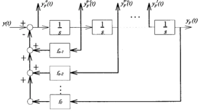
There remains one problem to resolve before the appli-cation of the continuous-time parameter estimation. The time derivatives in the data vector ␺ are usually unavailable if only the signals u(t) and y (t) are measured. One way to overcome the difficulty is to use the state variable filter 共SVF兲.23_{It is a state representation of an nth-order low-pass} transfer function F(s), F共s兲⫽yF共s兲 y共s兲 ⫽ 1 f0⫹ f1s⫹¯⫹ fnsn , 共12兲

where yF(s) and y (s) represent the Laplace transform of the filtered output yF(t) and the original output y (t), respec-tively. It provides simultaneously the time derivatives 共with-out direct differentiation兲 and filtering of the noise 共Fig. 2兲. In the paper, we choose a fourth-order Butterworth filter with a cutoff frequency of 200 Hz.

After all the derivatives are obtained from the SVF, the RLS algorithm is employed to calculate the model param-eters ␪. Assume that the relationship between the model pa-rameters␪and the process coefficients␳ is

␪⫽ f共␳兲, 共13兲

or, in matrix form,

␪⫽Cz, 共14兲

where z is a function of ␳, i.e.,

z⫽g共␳兲. 共15兲

FIG. 1. Architecture of the model-based method for the fault diagnosis system.

Thus the process coefficients ␳ can be obtained from the inverse relationship

␳⫽ f⫺1_{共␪兲. 共16兲}

A useful alternative to the forgoing continuous-time pa-rameter algorithm is the discrete-time papa-rameter estimation algorithm. The discrete-time algorithm follows basically the same line as the continuous-time version, except that the data vector ␺ contains the present and past data samples instead of time derivatives. There is no need for the SVF processing in constructing the data. The advantage of the discrete-time algorithm lies in the fact that it accommodates better than the continuous-time version the high-order dynamics of more complicated systems that cannot be modeled as simple ro-tors.

B. Modeling of rotor dynamics

In the paper, we model the rotor systems in terms of lateral vibrations that reflect the rotor faults commonly en-countered in practical applications. A classical rotor model suited for this purpose is the Jeffcott model.24,25

The Jeffcott model illustrated in Fig. 3, consists of a massless circular shaft with a fixed rigid circular disc sup-ported by flexible bearings at the center of the shaft. The disc is mounted with its plane perpendicular to the shaft axis. Its mass center S has a radial offset e with the shaft center W. The disc is assumed to move only in the 1-2 plane. The movement of the shaft center W relative to the unloaded position is given by coordinates (y1, y2) and the angle of the disc position is given by␸. The position of the point S can be expressed as

z1⫽y1⫹e cos␸, 共17兲

z2⫽y2⫹e sin␸. 共18兲

Assume that the damping coefficients in directions 1 and 2 are d1 and d2, respectively, the stiffness of shaft is K, and two bearings have equal pairs of stiffness K1 and K2 in the directions 1 and 2, respectively. The total stiffness of the shaft and bearings is

K₁

⬘

⬘

The equations of motion共as functions of y1, y2, and␸兲 can be obtained from applying Newton’s second law in transla-tion and rotatransla-tion.

M y¨1⫹d1y˙1⫹K1

⬘

M y¨2⫹d2y˙2⫹K2

⬘

Ip␸¨⫹e共d1y˙1⫹K1

⬘

⬘

Ip is the polar moment of inertia of disc, and T(t) is the mechanical torque input. Assuming that y1 and y2 are mea-sured with reference to the equilibrium position, we can re-write Eqs. 共21兲 and 共22兲, adjusted with an angle offset ␸0 that is the angle between the reference point and the center of mass,

y¨⫹2␰1␻01y˙1⫹␻012y1⫽e关␸¨ sin共␸⫹␸0兲

⫹␸˙2cos共␸⫹␸0兲兴, 共24兲

y¨2⫹2␰2␻02y˙2⫹␻022y2⫽e关⫺␸¨ cos共␸⫹␸0兲

⫹␸˙2sin共␸⫹␸0兲兴. 共25兲 Or,

y¨1⫹2␰1␻01y˙1⫹␻012y₁⫽e cos␸0共␸¨ sin␸⫹␸˙2_cos␸兲 ⫹e sin␸0共␸¨ cos␸⫺␸˙2sin␸兲,

共26兲

y¨2⫹2␰2␻02y2⫹␻022y2⫽e cos␸0共⫺␸¨ cos␸⫹␸˙2sin␸兲 ⫹e sin␸0共␸¨ sin␸⫹␸˙2cos␸兲,

共27兲 where ␻0i⫽

冑

⬘

冑

⬘

Equations 共26兲 and 共27兲 form the basis of the continuous-time parameter estimation which can be recast into the linear regression forms yi共k兲⫽␺i T_共k兲␪ i共k兲, i⫽1,2, 共30兲 where ␺1 T_{共k⫺1兲⫽关y¨}

1y˙1␸¨ sin␸⫹␸˙2cos␸␸¨ cos␸⫺␸˙2sin␸兴, 共31兲 ␺2

T_{共k⫺1兲⫽关y¨}

2y˙2␸˙2sin␸⫺␸¨ cos␸␸¨ sin␸⫹␸˙2cos␸兴, 共32兲 ␪1 T_{共k兲⫽关⫺a11⫺a21} b11b21兴, 共33兲 ␪2 T_{共k兲⫽关⫺a12⫺a22} b12b22兴, 共34兲 and FIG. 3. The Jeffcott rotor model with flexible bearings.

a1i⫽1/␻0i2, a2i⫽2␰i/␻0i, b11⫽b12⫽e cos␸0, 共35兲

b21⫽b22⫽e sin␸0.

From the model parameters, the process coefficients can be recovered as ␻0i⫽

_冑

冑

冑

冑

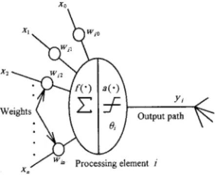
II. INTELLIGENT INFERENCE ALGORITHMS FOR FDI In the paper, artificial neural network and fuzzy theory are utilized for inference of rotor faults. Figure 4 shows a mathematical model of the biological neuron, usually called an M - P neuron,26,27where the ith processing element com-putes a weighted sum of its inputs x0,x1,x2,...,xn and out-puts yi⫽1 共firing兲 or 0 共not firing兲 according to whether this weighted input sum is above or below a certain threshold␪i,

yi共k⫹1兲⫽a共 f 兲

兺

n

wi jxi共k兲⫺␪i, 共39兲

where k is the iteration index of input and output and the activation function a( f ) is a unit step function,

a共 f 兲⫽

再

1, if f⭓0

0, otherwise. 共40兲

In the paper, the supervised learning network with back-propagation is employed. The algorithm generally includes two phases: the learning共training兲 process and the recall pro-cess. In the supervised learning, the objective is to reduce the error between the desired output and the calculated output. To quantify the quality of learning, an error function is uti-lized,

E⫽1

2

兺

2_{, 共41兲}

where Tiis the desired output vector and Aiis the calculated output vector. Methods such as the gradient search algorithm can be used for finding the minimum of E. In the training phase, the network weightings are updated according to the

sensitivity of the error function with respect to the weight-ings

⌬wi j

n_⫽⫺␩ ⳵E

⳵w_{i j}n , 共42兲

where ⌬w_{i j}n is the increment of the weighting between the

ith processing element of the (n⫺1)th layer and the jth

processing element of the nth layer, and␩is the step size for the gradient search algorithm.

Since Zadeh introduced in 1965 the fuzzy sets to repre-sent vagueness of linguistics, a rapid growth in the use of fuzzy theories is witnessed in many scientific applications.26 In contrast to classical sets that are crisp sets based on the binary logic 共‘‘Truth’’ or ‘‘False’’兲, the fuzzy sets are not only to classify one element belonging to a set or not, but to fuzzify in ‘‘Truth’’ with some degree of membership. Let A˜ be a fuzzy set and U be its universe of discourse

A

˜_{⫽兵共x,␮}

A

˜共x兲兲兩x苸U其_, 共43兲

where␮A˜(x) is the membership function of x in the fuzzy set

A

˜ that represents the degree of x belonging to the fuzzy set A

˜ , and its value is usually in the interval 关0, 1兴. A general architecture of a fuzzy logic control共FLC兲 system including a fuzzifier, a fuzzy rule base, an inference engine, and a defuzzifier, is shown in Fig. 5. If the output from the defuzzi-fier is not a control action 共as in our case兲 for a plant, the system becomes a fuzzy logic decision system.

In this study, a Self-cOnstructing Neural Fuzzy Infer-ence Network 共SONFIN兲, which is inherently a fuzzy rule-based model possessing neural network,26 is employed for intelligent inference and isolation of faults. This technique integrates the advantages of both artificial neural network and the fuzzy theory, and is well suited for automatic infer-ence required in the FDI application. The structure of the SONFIN is shown in Fig. 6, whereby the network consists of six layers: the input layer, the membership layer, the fuzzy rule layer, the normalization layer, the consequent layer, and the output layer. The network realizes the following fuzzy model:

Rule i: IF 共x1 is Ai1 and¯and xn is Ain兲

THEN 共y is m0i⫹a_jix_j⫹¯兲, 共44兲

where Ai j is a fuzzy set, m0i is the center of a symmetric membership function on y, and aji is a consequent param-eter. There are no rules initially, but they are created and adapted as on-line learning proceeds via simultaneous struc-ture and parameter identification. The learning process in-volves four steps: input/output space partitioning, construc-FIG. 4. A schematic diagram of a McCulloch–Pitts neuron共Ref. 26兲.

tion of fuzzy rules, optimal consequent structure identification, and parameter identification. The first three steps are for structure learning and the last step for parameter learning. In the structure identification of the precondition part, the input space is partitioned by using an aligned clustering-based algorithm, while in the structure identifica-tion of the consequent part only a single value selected by a clustering method is assigned to each rule initially.

After-wards, some additional significant input variables selected via the Gram–Schmidt orthogonalization for each rule will be added to the consequent part incrementally. Furthermore, to enhance the knowledge representation, a linear transfor-mation for each input variable is incorporated into the net-work so that fewer rules are needed. Finally, in parameter identification, the RLS algorithm is used to tune the param-eters in layer 5 and the back-propagation algorithm is used to update the parameters of the membership functions in layer 2. The trained neural fuzzy network is used for the subse-quent inference for faults. The unique features of SONFIN are twofold. First, the structure and the weights of the net-work are automatically adjusted. Second, a high-dimensional fuzzy system is implemented with a small number of rules and fuzzy terms. Due to the physical meaning of the fuzzy if–then rule, each input node in the SONFIN is only con-nected to its related rule nodes through its term nodes, in-stead of being connected to all the rule nodes in layer 3. This results in a small number of weights to be tuned. In some cases, however, it is time consuming to train the network provided the number of inputs is large. To alleviate the dif-ficulty, a Discriminatory Information 共DI兲 method4 can be FIG. 6. Structure of the Self cOnstructing Neural Fuzzy Inference Network

共SONFIN兲. In the figure, x’s are input variables; R’s are fuzzy rules; a’s are weightings in back-propagation.

FIG. 7. Schematic of the discriminatory information共DI兲 method. 共a兲 A more discriminatory feature;共b兲 a less discriminatory feature.

FIG. 8. Experimental arrangement of the rotor kit.

FIG. 9. The time variation of e in the normal, imbalanced, looseness, and faulty bearing conditions of the rotor kit. Normal: ——, imbalanced:•• , looseness: –•–, and faulty bearing: --.

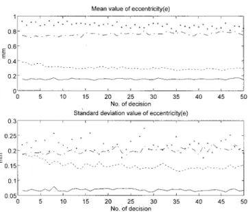
used to calculate the statistics of the data and retain only the inputs that account for the distinct features associated with the different conditions. The basic idea of the DI method is to choose the features that have distributions of distinct means and small spreads with respect to different conditions. The procedure is summarized as follows:

共a兲 A test is performed to collect 128 samples of system parameters, e.g., eccentricity, damping ratio, natural frequency, etc.

共b兲 Probability density functions 共pdf兲 are calculated for the extracted parameters in an off-line manner. 共c兲 If the mean value deviates from the normal case by

20% and the ‘‘2-␴’’ regions do not overlap, then the parameter is considered a good discriminator for the fault type of interest and thus serves as an input vari-able to the network. Otherwise, the parameter is dis-carded.

An example of the use of the DI method is shown in Fig. 7. The feature of Fig. 7共a兲 shows more isolated mean values and smaller variances than that of Fig. 7共b兲. Thus the former feature is preferably used as the principal input to the net-work.

III. EXPERIMENTAL INVESTIGATIONS

Experiments were carried out to validate the proposed FDI technique. In particular, we verified the feature genera-tion and fault inference algorithm by using a rotor kit that is capable of producing common rotor faults. Then, a centrifu-gal fan was also used to justify the practicality of the FDI system.

A. Rotor kit

A rotor kit is used in the first part of the experiments 共Fig. 8兲. The rotor kit consists of a constant-speed 共1500 rpm兲 induction motor, a coupling, a steel shaft, two ball-bearing supports, an aluminum disk, and a disturbance motor module. Five common rotor faults, imbalance, misalignment, disturbance, mechanical looseness, and faulty bearings can be conveniently produced by the rotor kit. Imbalance is cre-ated by adding an imbalanced weight on the disk. Misalign-ment is created by dislocating the coupling with a radial offset. Disturbance is created by a frictional disk driven by another induction motor running at a different angular fre-quency. The mechanical looseness is created by loosening one of the four bolts at the two bearing supports. The bearing fault is created by using a damaged outer ring. On the other hand, the FDI system consists of two eddy-current probes, a photo switch 共for angular frequency measurement兲, and a personal computer equipped with a DSP card共TMS320C32兲 and 32 analog I/O channels.

In case 1, the FDI method based on continuous-time parameter estimation is investigated. Lateral displacements in both horizontal and vertical directions near the center of the disc are measured by two eddy-current probes. The an-gular velocity ⍀ is measured by a photo switch. The mea-sured signals are fed to the DSP via the analog I/O module with a sampling rate 200 Hz. Using the SVF method, the time derivatives of displacements are calculated. Based on the data, the continuous-time RLS algorithm is employed to generate the features including five process coefficients. The DI procedure is used to preprocess the features and remove the insignificant inputs. These data features then become the input vector to the neural fuzzy network. In the first 共train-ing兲 stage of 12-sec measurement, five types of fault and the normal condition are produced by the rotor kit, and the data features are calculated to train the neural fuzzy network. In the second共recall兲 stage, the rotor is restarted for five times and for each time the faults are regenerated to verify the trained network. Each time record is further divided into ten sets to represent ten experiments. There are altogether 6⫻5 ⫻10⫽300 experiments. Figure 9 shows the variations of e in the normal, imbalanced, mechanical looseness, and faulty bearing conditions, respectively, of the rotor kit. The varia-tions of the other process coefficients in the other condivaria-tions during an ongoing experiment are similarly calculated. The effects of five types of fault on the estimated process coeffi-cients for the rotor kit are summarized in Table I.

Appar-TABLE I. Effects of different faults on the estimated continuous-time pro-cess coefficients for the rotor kit. 共x¯: average;␴: standard deviation;⫹: increase;⫺: decrease;*: insignificant兲.

Parameters Condition x ¯ of ␻01 x ¯ of ␻02 x ¯ of ␰1 x ¯ of ␰2 x ¯ of e ␴of ␻01 ␴of ␻02 ␴of ␰1 ␴of ␰2 ␴of e Disturbance ⫺ ⫺ * _⫹ * _{⫹ ⫹ ⫹ ⫹ ⫹} Imbalance ⫹ * _⫺ * _{⫹ ⫹} * _⫺ * _⫹ Misalignment ⫹ ⫹ ⫹ ⫹ ⫹ ⫹ ⫹ ⫹ ⫹ ⫹ Looseness * ⫺ ⫺ ⫺ ⫺ * * ⫺ ⫺ ⫺ Faulty bearing ⫺ * ⫹ * * ⫹ * ⫹ * ⫹

TABLE II. Performance of the continuous-time model-based FDI technique for the rotor kit. Condition

Result Normal Disturbance Imbalance Misalignment Looseness Faulty bearing

Normal 100% 0% 0% 0% 0% 0% Disturbance 0% 92% 0% 0% 0% 0% Imbalance 0% 8% 100% 0% 0% 0% Misalignment 0% 0% 0% 100% 2% 0% Looseness 0% 0% 0% 0% 98% 8% Faulty bearing 0% 0% 0% 0% 0% 92%

ently, it is very difficult for an experienced operator to detect and isolate the fault by merely looking at the trends in the table. This calls for the capability of automatic machine-learning of the neural fuzzy network. Table II summarizes the performance of the continuous-time FDI technique with neural fuzzy inference for the rotor kit. The result appears acceptable共average rate of correct inference⫽97%兲.

In case 2, the FDI technique based on discrete-time pa-rameter estimation is examined. The foregoing assumption that the angular frequency is constant is relaxed. It is as-sumed that the discrete-time model of the rotor system is of the form

y1共k兲⫽⫺a1iy1共k⫺1兲⫺a2iy1共k⫺2兲

⫹b1i␻˙ cos共␻k兲⫹b2i␻˙ cos共␻共k⫺1兲兲

⫹b3i␻˙ sin共␻k兲⫹b4i␻˙ sin共␻共k⫺1兲兲,

i⫽1,2, 共45兲

where a’s and b’s are model parameters to be determined and ␻˙ is the time derivative of␻that is calculated by the SVF. The above equations can be cast into the linear regression form y (k)⫽␺T(k)␪(k) with the data vectors

⌿i

T_{共k⫺1兲⫽关y}

i共k⫺1兲yi共k⫺2兲␻˙ cos共␻k兲␻˙ ⫻cos共␻共k⫺1兲兲␻˙ sin共␻k兲

⫻␻˙ sin共␻共k⫺1兲兲兴, i⫽1,2, 共46兲

and the parameter vectors ␪i

T_{共k兲⫽关⫺a1i⫺a2ib}

1ib2ib3ib4i兴. 共47兲

Other than the parameter estimation model, the experi-mental setup remains the same as in the continuous-time case. The discrete-time parameter estimation algorithm is employed to generate the features that in turn become the input vectors to the neural fuzzy inference network. Follow-ing a procedure similar to the continuous-time algorithm, the neural fuzzy network is necessary to infer the fault types, based on the features 共model parameters in this case兲 ex-tracted earlier by the discrete-time RLS algorithm. Table III summarizes the performance of the discrete-time FDI tech-nique with neural fuzzy inference for the rotor kit. In com-parison with the continuous-time method, the result appears to be slightly improved 共average rate of correct inference ⫽99.0%兲.

B. Centrifugal fan

A more practical system, a two-horsepower centrifugal fan, is chosen for validating the proposed FDI technique. The experimental setup including the fan and the FDI system is shown in Fig. 10. The fan system consists of a constant-speed 共1750 rpm兲 AC induction motor, a steel shaft, a cou-pling, two bearing supports, and 12 impellers. Four common faults of centrifugal fans, including imbalance, misalign-ment, mechanical looseness, and faulty bearing are

investi-FIG. 10. Experimental arrangement of the centrifugal fan.

FIG. 11. The time variation of e in the normal, imbalanced, looseness, and faulty bearing conditions of the centrifugal fan. Normal: ——, imbalanced: •• , looseness: –•–, and faulty bearing: --.

TABLE III. Performance of the discrete-time model-based FDI technique model for the rotor kit. Condition

Result Normal Disturbance Imbalance Misalignment Looseness Faulty bearing

Normal 100% 0% 0% 0% 0% 0% Disturbance 0% 100% 0% 0% 0% 0% Imbalance 0% 0% 98% 0% 0% 0% Misalignment 0% 0% 0% 96% 0% 0% Looseness 0% 0% 2% 4% 100% 0% Faulty bearing 0% 0% 0% 0% 0% 100%

gated in the experiment. The faults are created the same way as the earlier procedures in rotor kit, except that the faulty bearing was replaced with a lubricated bearing.

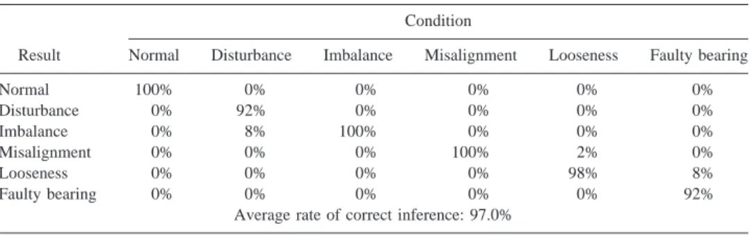
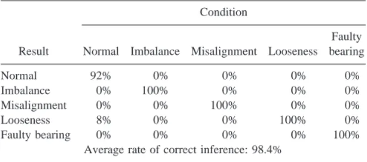
In case 1, the FDI technique based on continuous-time parameter estimation is examined. Lateral displacements in both horizontal and vertical directions near the impellers are measured by two eddy-current probes. The angular velocity ⍀ is measured by the photo switch. The other conditions are the same as in case 1 of the rotor kit. Following a procedure similar to the continuous-time algorithm, the neural fuzzy network is necessary to infer the fault types, based on the features extracted earlier by the RLS algorithm. Figure 11 shows the variations of e in the normal, imbalanced, me-chanical looseness, and faulty bearing conditions, respec-tively. The neural fuzzy network is used to infer the fault types, based on the features共process coefficients in this case兲 extracted earlier by the continuous-time RLS algorithm. Table IV summarizes the performance of the continuous-time FDI technique with neural fuzzy inference for the cen-trifugal fan. The result appears acceptable 共average rate of correct inference⫽98.4%兲.

In case 2, the FDI method based on the discrete-time parameter estimation technique is examined. The foregoing assumption that the angular frequency is constant is relaxed. The other conditions remain unchanged from case 2 of the rotor kit. Following a procedure similar to the continuous-time algorithm, the neural fuzzy network is necessary to in-fer the fault types, based on the features extracted earlier by the RLS algorithm. Table V summarizes the performance of the discrete-time FDI technique with neural fuzzy inference for the centrifugal fan. Compared to the continuous-time method, the result appears excellent共average rate of correct inference⫽100.0%兲. It is noted from Tables II–V that the

‘‘false alarm’’ rates and ‘‘failure-to-alarm’’ rates are all zero except the case of the centrifugal fan, where 8% of the data under ‘‘normal’’ conditions are misinterpreted as looseness faults. In these experiments, 97% detection rate is considered sufficient.

IV. CONCLUDING REMARKS

An on-line FDI system for rotator vibration is presented. The development of the proposed methods is divided into two stages. First, data features are generated based on two model-based methods. Second, fault types are determined based on the extracted features via neural fuzzy inference algorithms. The proposed FDI system is implemented on a DSP. The usefulness of the proposed technique in identifying common rotor faults has been justified by experiments con-ducted for a rotor kit and a centrifugal fan. From the experi-mental results, the discrete-time parameter estimation ap-proach that does not require analytical modeling of the system yields better performance than the continuous-time approach. However, the success of the methods hinges on the proper choices of the model structures.

The proposed FDI technique can readily be extended to other systems such as centrifugal pumps, centrifugal com-pressors, and machine tools. The system will be extended for handling multiple faults. In practical applications, informa-tion is generally incomplete. The machine condiinforma-tion is gen-erally unknown so that the field data are insufficient for re-liable training of the network. Thus enhancing the present neural fuzzy inference network, in light of machine learning and human knowledge, for an expert system suited for robust FDI will be the focus of future research.

ACKNOWLEDGMENTS

Special thanks go to Dr. G. H. Chen for the helpful discussions on the FDI subject. The work was supported by the Institute of Occupational Safety and Health 共IOSH兲, Council of Labor Affairs, Executive Yuan in Taiwan, Re-public of China, under the project ‘‘Development of Hazard-Preventive Techniques of Major Hydraulic Machinery.’’

1_{P. M. Frank, ‘‘Fault diagnosis in dynamic systems using analytical and}

knowledge-based redundancy—A survey and some new results,’’ Auto-matica 26, No. 3, 459–474共1990兲.

2_{S. J. Mitchell, Machinery Analysis and Monitoring 共Penn Well,}

Okla-homa, 1981兲.

3_{J. E. Berry, ‘‘Proven method for specifying both spectral alarm bands as}

well as narrowband alarm envelopes using today’s predictive maintenance software system,’’ BandAid Technical Literature, Technical Associates of Charlotte, Inc., Charlotte, NC, 1993.

4_{S. Braun, Mechanical Signature Analysis—Theory and Applications}

共Aca-demic, Orlando, Florida, 1986兲.

5

H. Kumamoto, ‘‘Application of expert system techniques to fault diagno-sis,’’ Chem. Eng. J. 29, 1–9共1984兲.

6_{R. L. Actis and A. D. Dimarogonas, ‘‘Non-linear effects due to closing}

cracks in vibrating beams,’’ ASME Des. Eng. Div. Publ. DE Struct. Vib. Acoust. 18, 99–104共1989兲.

7_{J. Wauer, ‘‘On the dynamics of cracked rotors: A literature survey,’’}

Appl. Mech. Rev. 43, 13–17共1990兲.

8_{X. T. C. Man, L. M. McClure, Z. Wang, and R. D. Finch, ‘‘Slot depth}

resolution in vibration signature monitoring of beams using frequency shift,’’ J. Acoust. Soc. Am. 95, 2029–2037共1994兲.

9_{X. T. C. Man and R. D. Finch, ‘‘Vibration monitoring of slotted beams}

using an analytical model,’’ J. Acoust. Soc. Am. 102, 382–390共1997兲. TABLE IV. Performance of the continuous-time model-based FDI

tech-nique for the centrifugal fan.

Condition

Result Normal Imbalance Misalignment Looseness Faulty bearing Normal 92% 0% 0% 0% 0% Imbalance 0% 100% 0% 0% 0% Misalignment 0% 0% 100% 0% 0% Looseness 8% 0% 0% 100% 0% Faulty bearing 0% 0% 0% 0% 100%

Average rate of correct inference: 98.4%

TABLE V. Performance of the discrete-time model-based FDI technique for the centrifugal fan.

Condition

Result Normal Imbalance Misalignment Looseness Faulty bearing Normal 100% 0% 0% 0% 0% Imbalance 0% 100% 0% 0% 0% Misalignment 0% 0% 100% 0% 0% Looseness 0% 0% 0% 100% 0% Faulty bearing 0% 0% 0% 0% 100%

10_{R. Isermann, ‘‘Fault diagnosis of machines via parameter estimation and}

knowledge processing—tutorial paper,’’ Automatica 29, No. 4, 815–835

共1993兲.

11

C. F. Juang and C. T. Lin, ‘‘An on-line self-constructing neural fuzzy inference network and its applications,’’ IEEE Trans. Fuzzy Systems 6, No. 1,12–13共1998兲.

12_{P. M. Frank, ‘‘Analytical and qualitative model-based fault diagnosis—A}

survey and some new results,’’ European J. Control 2, 6–28共1996兲.

13

R. Isermann, ‘‘Process fault detection based on modeling and estimation methods—A survey,’’ Automatica 20, No. 4, 387–404共1984兲.

14_{R. Isermann, ‘‘Process fault diagnosis based on process model}

knowledge—Part I. Principles for fault diagnosis with parameter estima-tion,’’ J. Dyn. Syst., Meas., Control 113, No. DEC, 620–626共1991兲.

15_{R. Isermann, ‘‘Process fault diagnosis based on process model}

knowledge—Part II: Principles for fault diagnosis with parameter estima-tion,’’ J. Dyn. Syst., Meas., Control 113, No. DEC, 627–633共1991兲.

16_{R. Isermann, ‘‘Estimation of physical parameters for dynamic processes}

with application to an industrial robot,’’ Int. J. Control 55, No. 6, 1287– 1298共1992兲.

17_{K. L. Jones, ‘‘Failure detection in linear systems,’’ The Charles Stark}

Draper Laboratory, Cambridge, MA, Rep. T-608.

18

E. Y. Chow and A. S. Willsky, ‘‘Analytical redundancy and the design of

robust failure detection systems,’’ IEEE Trans. Autom. Control. AC-29, No. 7, 603–614共1984兲.

19_{J. Gertler, ‘‘Residual generation in model-based fault diagnosis,’’ Control}

Theory Advanced Technology 9, No. 1, 259–285共1993兲.

20_{R. J. Patton and J. Chen, ‘‘Robust fault detection of jet engine sensor}

systems using eigenstructure assignment,’’ J. Guid. Control. Dyn. 15, No. 6, 1491–1497共1992兲.

21

L. Ljung, System Identification: Theory for the User共Prentice-Hall, Engle-wood Cliffs, NJ, 1987兲.

22

G. C. Goodwin and K. S. Sin, Adaptive Filtering Prediction and Control

共Prentice-Hall, Englewood Cliffs, NJ, 1984兲.

23

P. C. Young, ‘‘Parameter estimation for continuous-time models—A sur-vey,’’ Automatica 17, 23–39共1981兲.

24

Handbook of Rotordynamics, edited by E. F. Ehrich共McGraw-Hill, New

Delhi, India, 1992兲.

25_{K. Erwin, Dynamics of Rotors and Foundations共Springer-Verlag, Berlin,}

1993兲.

26_{C. T. Lin and Lee C. S. George, Neural Fuzzy Systems共Prentice-Hall,}

Englewood Cliffs, NJ, 1996兲.

27

T. Kohonen, ‘‘An introduction to neural computing,’’ Neural Networks 1, 3–16共1988兲.