Abstract—In this paper, a probability-based segmentation approach is presented for object tracking. The proposed approach uses the Dirichlet process mixture model to describe the probabilistic distribution of observations in a single scan of a laserscanner. Then the number of segments is inferred from the observations by the Gibbs sampling method. Moreover each segment is classified into one of the three predefined classes such that most of non-vehicle-like objects on the roadsides can be filtered out. Then, the tracking algorithm, called Joint Integrated Probabilistic Data Association Filter (JIPDAF), is applied to track the classified objects and manage existing tracks. Simulations based on real traffic data demonstrate that the non-vehicle-like objects on the roadsides are suppressed. Since the number of objects in the tracking step is decreased, the computation load of the tracking step is decreased.
I. INTRODUCTION
In today’s automotive industry, various driver assistance systems have been developed to enhance driving safety and alleviate driver workload. The correct operations of these systems rely on the ability to detect and track objects around the vehicle. Radar, laserscanner and video camera are commonly used for this purpose. The laserscanner has the advantage of the high angle and radial resolution and it preserves the geometric information about the objects. Therefore the process of object detecting and tracking based on the laserscanner consists of three steps: segmentation, classification and tracking. Segmentation is a process of grouping together the observations from the same object in a given scan and then each segment is classified into one of several different classes in the classification step. Finally, the tracking step associates segments representing the same object from scan to scan.
Several distance-based approaches have been developed to segment the observations in a given scan, e.g., [1][2][3]. The segmentation results of these distance-based methods depend on the chosen threshold [4]. In order to separate spatially closed objects, the threshold is chosen to be small, which could lead to an excessive number of segments and thus This work was partially supported by the Industrial Technology Research Institute and the Department of Industrial Technology, Ministry of Economic Affairs, Taiwan under the grant number 98-EC-17-A-19-S2-0052.
Tesheng Hsiao is with the National Chiao Tung University, 300 Hsinchu, Taiwan ( phone: 886-3-571-2121#31249; fax: 886-3-5715998; e-mail: [email protected] ).
Yung-Chou Lee is with the National Chiao Tung University, 300 Hsinchu, Taiwan ( e-mail: [email protected] ).
.
increases the computation load of the tracking step as a consequence. This situation becomes manifest when the own vehicle is driven on urban streets. The observations of the static objects usually cluttered up the roadsides and are difficult to be segmented properly. Nearby observations from two objects could be grouped into one segment if a large threshold is used. Therefore, tuning the threshold is a tradeoff. As an alternative to these distance-based segmentation methods, we consider a probability-based segmentation approach to reduce the number of segments on the roadsides; meanwhile, the observations in front of the own vehicle could be segmented correctly. The Dirichlet process (DP) mixture model is used to describe the probabilistic distribution of observations in each scan of the laserscanner because of the flexibility of the DP mixture model in dealing with segmentation [5]. The number of segments in the DP mixture model is inferred from observations by the Gibbs sampling method. The segmentation results depend on the spatial distribution of the observations in each scan.
Following the segmentation step, each segment is classified into one of several predefined classes. In this paper, only three classes, which are small, medium, and big objects, are defined. The tracks which are initialized from the non-vehicle-like objects on the roadsides can be suppressed by excluding the big objects in the tracking step. Then, a track is initialized for small or medium object in the tracking step. The Joint Integrated Probabilistic Data Association Filter (JIPDAF) algorithm [7] is used to update the tracks and calculate the existence probability of every track. The track management, which includes the track confirmation and track deletion, is implemented based on this probability.
The paper structure is shown as follows: Sections II and III describe the modules of scan segmentation and object classification. The object tracking is presented in section IV. Finally some results of simulations and conclusions are presented in sections V and VI, respectively.
II. SCAN SEGMENTATION
A. Dirichlet Process Mixture Model
The purpose of the scan segmentation is to group all the observations of a scan into several segments, each of which represents an individual object. Since the number of segments is unknown, the proposed method uses the DP mixture model to describe the probabilistic distribution of the observations
Object Tracking via the Probability-Based Segmentation Using Laser
Range Images
and then performs probabilistic inference about the segments. A Dirichlet process defines a distribution over probability measures on potentially infinite parameter spaces Θ. This stochastic process, DP(α0, G0), is defined by a positive real
number, α0, and a base measure, G0. The stick-breaking
construction of DP [8] is given below
(
)
(
)
0 0 0 0 0 0 1 1 1 | , G ~ beta 1, , | ,G ~ G , 1 , G k k k k k k l l k k φ π α α φ α π π − π ∞ π δ = = ′ ′ ′ =∏
− =∑
(1)where beta(1,α0) is the beta distribution with parameters 1
and α0. The sequenceπ
( )
πk k 1∞ = = constructed by (1) satisfies 1πk 1 ∞ =
∑
with probability one. The random measure G is distributed according to DP(α0, G0). Suppose that observationxi arise as
( )
| G ~ G, | ~ , i i i i x F θ θ θ (2) where F(θi) denotes the distribution of the observation xiwith parameter θi. The factors θi are assumed to be random
variables and are conditionally independent given G, and the observation xi is conditionally independent of the other
observations given the factor θi. When G is distributed
according to a DP, this model is referred to as a DP mixture model. A graphical model representation of a DP mixture model is shown in Fig. 1(a) [8]. An equivalent representation of a DP mixture model using a stick-breaking construction is given by the following conditional distributions [5]:
( )
( )
( )
0 0 0 0 1 | ~ GEM , | ~ , | G ~ G , | , ~ i i k i i k k z z x z F π α α π π φ φ ∞= φ (3)where GEM means that π is constructed by (1) and the factors θi take on values φk with probability πk. An alternative
graphical model using a stick-breaking construction is shown in Fig. 1(b). A tutorial on DP can be found in [8].
In this paper, the object tracking is implemented in Cartesian coordinates. The ith observation, x
i = (xi, yi), is
distributed according to N(μi, Σi), where μi is the mean vector
and Σi is the covariance matrix. In other words,
xi|θi ~ N(μi, Σi), θi={ μi, Σi }
Figure 1. (a) Graphical representation of Dirichlet process mixture model. (b) Alternative representation using a stick-breaking construction.
Each observation is associated with an indicator variable zi,
which represents the segment number. A conjugate normal-inverse-Wishart prior, denoted byNIW
(
κ ϑ ν, , ,Δ)
, on θi is placed and takes the following form:(
)
(
)
(
)
(
)
1 1 1 2 , | , , , 1 exp 2 2 i i d T i i i i i p tr ν μ κ ϑ ν κ ν μ ϑ μ ϑ + ⎛ ⎞ −⎜⎝ +⎟⎠ − − Σ Δ ⎧ ⎫ ∝ Σ ⎨− ΔΣ − − Σ − ⎬ ⎩ ⎭ (4) where d is the dimension of x, ν and Δare the degrees of freedom and covariance parameter for the inverse-Wishart density, ϑ is the expected mean, and κ is the number of pseudo-observations. The parametersκ , ϑ ,ν and Δ are called the prior hyperparameters λ . In order to infer the indicator variable zi, aGibbs sampler by marginalizing overthe infinite set of parameters θ and mixture weights π as in [9] is used. Given the assignments
{ }
1
N j j
z= z = from the last iteration, the posterior distribution of zi factors for the Gibbs
sampling as follows:
(
i| \i, , ,)
(
i| \i,) (
i| , \i,)
p z z xλ α ∝p z z α p x z x λ (5) If \{
}
1 | N i j jz = z j i≠ = forms K clusters, and assigns \i
k
N observations to the kth cluster, the new cluster assignment
zi are sampled from the following (K+1)-dimension
multinomial:
(
)
( ) (
)
( ) (
)
\ \ 1 | , , , 1 , , 1 i i K i k k i i new i i k p z z x N f x z k f x z K C λ α δ α δ = ⎛ ⎞ = ⎜⎜ + + ⎟⎟ ⎝∑
⎠ (6) where( )
(
)
(
)
(
)(
)
( ) 2 1 2 1 2 1 1 k i T i i f x x x ν ν κ ν ν κ π κ ν ϑ ϑ κ + − Δ = + Δ + − − +( )
(
)
(
)
(
)(
)
( ) 2 1 2 1 2 1 1 new i T i i f x x x ν ν κ ν ν κ π κ ν ϑ ϑ κ + − Δ = + Δ + − − +{
}
{
}
( )
( )
\ 1 \ 1 \ 1 | , = + | + - , = + N i j j k j N T T T i j j j k j K i k k i new i k x z k N x x z k N C N f x f x κϑ κϑ κ κ ν ν κϑϑ κϑϑ ν ν α = = = = + = Δ = Δ + = = +∑
∑
∑
The Gibbs sampler based on (6) is used to resample the N cluster assignments zi in order and update fk(x) for each new
sampled assignment zi. A new cluster is created when zi is
equal to K+1 and a cluster is deleted if none of the observations are assigned to this cluster.
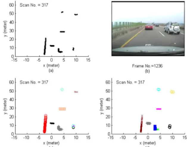
Fig. 2(c) and 2(d) show the segmentation results using the distance-based approach [1] and the probability-based
approach, respectively. The threshold, S0, used for noise reduction for the distance-based approach is 1.5 and the parameters for the probability-based approach are listed in section V. The number of segments in Figure 2(d) is smaller than that in Figure 2(c); therefore the number of tracks which need processing is reduced. The tracking results are shown in section V. Figure 3(d) shows that the right-angle shape “|_” (“_|”) which represents the rear and left (right) sides of a vehicle, is separated into two segments due to the Gaussian assumption of the observations used in the DP mixture model. Therefore, these two segments need to be grouped into one. Besides, segments of the same object separated due to occlusions are also grouped by the following grouping method.
A. Joint Broken Segments
The main purpose of this procedure is to group the broken segments due to the right-angle shape and the obscuration of the security barrier on the highway. Since both distance-
Figure 2. The results of segmentation when driving on a road. (a) The original observation in one single scan. (b) The corresponding video frame. (c) The segmentation result of the distance-based approach. (d) The segmentation result of the probability-based approach.
Figure 3. The results of segmentation when driving on a highway. (a) The original observation in one single scan. (b) The corresponding video frame. (c) The segmentation result of the distance-based approach. (d) The segmentation result of the probability-based approach.
based and probability-based methods result in broken segments, it is required to group these broken segments before the classification step. First of all, we count the observation from right to left and assign an order number i to each observation. So the bearing of the first observation is 40 degree, as shown in Fig. 4. The angular resolution of the laserscanner is configured to be 0.5 degrees. The maximum number of observations in a scan is 201 (i =1~201). Similarly, each segment is assigned a number s with the order from right to left. Two segments sth and (s+1)th, which form a right-angle
shape are grouped together as long as the following conditions are fulfilled:
( ) ( ) ( ) ( )
max , min , 1 max , min , 1
x i s−x i s+ <0.5, y i s−y i s+ <2.5 (7) where xmax(i),s means the x value of the maximum order
number in the sth segment and x
min(i),s means the x value of the
minimum order number in the sth segment. After grouping
the segments of right-angle shape, the broken segments of the security barrier, sth and (s+2)th, are grouped if the following
conditions are satisfied:
( ) ( ) ( ) ( )
max , min , 2 max , min , 2
x i s−x i s+ <0.5, y i s−y i s+ <20 (8) In order to avoid grouping the segments which represent different vehicles, (8) is not implemented if the number of the segments, after (7) is done, is bigger than ten.
III. OBJECT CLASSIFICATION
In the object classification step, each segment is classified into one of the three predefined classes according to the size of the segment. The size of the segment is determined as follows:
( )
( )
( )
( )
x , , y , ,
b = max xi s −min xi s , b = max yi s −min yi s Next, a representative point of each object, called the measurement vector, is calculated and used for object tracking.
A. Predefined Classes
Let the size of the segment be (bx, by) and the three classes
of the objects are defined as follows:
• Small object: bx≦0.8m and by≦1.2m
• Medium object: 0.8m<bx≦3m and 1.2m<by≦12m
• Big object: 3m<bx or 12m<by
The small objects such as pedestrians, bicycles, and scooters are vulnerable in a car accident. Therefore, the object tracks for the small objects in section V are plotted by the red color. The medium objects include cars, trucks, and buses and the big objects include walls and security barriers. If the segment is classified as a big object, it is excluded from updating tracks. Removing the big objects can benefit the tracking algorithm by focusing on tracking the other dangerous objects on the road.
B. Obtaining the Measurement Vector
The measurement vector for the sth segment, denoted by
moving direction of the object is the same as the own vehicle. On the other hand, the middle-front of the object is chosen as the measurement vector in the case of opposite moving direction. However, it is hard to find the measurement vector correctly through the segment which captures only partial information about the geometry and size of the real object. Therefore a heuristic method is applied to the following four typical kinds of segments.
• “-” shape: m m ., ., (x , y ) average(x , y )s s = s s • “|_” shape: min m m , , 1, , (x , y ) average(x , y ), s s = l s l s l i= s, ,K ir s • “_|” shape: min m m , , , end, (x , y ) average(x , y ), s s = l s l s l i= r s, ,K i s • “ | ” shape:
( )
( )
(
)
m m ., ., (x , y )s s = average x s , minimum y swhere x.,s means all observations in x-direction belong to the sth segment, i
1,s and iend,s denote the minimum and
maximum order number of the observations in the sth segment,
and irmin,s denotes the order number of the observation with the minimum range in the sth segment.
IV. OBJECT TRACKING
An existing object is associated with a track which passes three phases during its existence: tentative, preliminary, and maintenance [10]. The JIPDAF gives the probability of track existence with two propagation models, Markov chain one and Markov chain two [7]. Markov chain one defines the probability of track existence at scan k asP x
{ }
k and is given by{ }
{ }
(
{ }
)
{ }
{ }
(
{ }
)
1 1 11 1 21 1 1 1 21 1 22 1 1 1 1 k k k k k k P x p P x p P x P x p P x p P x − − − − = + − − = + − (9)The Markov chain two separates the probability of track existence at scan k into the observable track
{ }
ok
P x and the non-observable track
{ }
nk
P x . The model for Markov chain
two is expressed as
{ }
{ }
{ }
(
{ }
)
{ }
{ }
{ }
(
{ }
)
{ }
{ }
{ }
(
{ }
)
2 2 2 11 1 21 1 31 1 2 2 2 12 1 22 1 32 1 2 2 2 13 1 23 1 33 1 1 1 1 = 1 o o n k k k k n o n k k k k o n k k k k P x p P x p P x p P x P x p P x p P x p P x P x p P x p P x p P x − − − − − − − − − = + + − = + + − − + + − (10) where{ }
{ } { }
o n k k kP x =P x +P x . For both models, the Markov chain coefficients must satisfy
1 1 1 1 11 12 21 22 2 2 2 2 2 2 2 2 2 11 12 13 21 22 23 31 32 33 1 1 p p p p p p p p p p p p p + = + = + + = + + = + + = (11)
The track management is implemented via the probability,
{ }
kP x .
A. Track Management 1) Tentative Track:
The unassociated measurement vectors become tentative tracks after the updates of maintenance and preliminary tracks are finished in the previous scan. A preliminary track is promoted from a tentative track using the two-point differencing method [11], i.e. the promotion occurs if any of the measurement vectors in the present scan are within a reasonable distance of a tentative track in the previous scan. If none of the measurement vectors initiate a new preliminary track for a particular tentative track, then the tentative track is deleted.
2) Preliminary Track:
The preliminary track is updated through the Markov chain one model. However, the Integrated Probabilistic Data Association Filter (IPDAF) [6] is used here to update the preliminary tracks because of the lower computation load. The IPDAF also gives the probability of track existence with the same two propagation models. Furthermore, JIPDAF and IPDAF integrate seamlessly with no transition effects when switching from one to the other [7]. Once the existence probability of a preliminary track reaches a specified level, the track is promoted to the maintenance track. Conversely, if the existence probability falls below another specified level, the preliminary track is deleted.
3) Maintenance Track:
Each maintenance track represents an object and the maintenance track is updated through the Markov chain two model of the JIPDAF. The track is deleted when the existence probability falls below the specified level. Besides, two maintenance tracks are merged if the distances of these two tracks in the x and y directions are less than 0.8m and 1.2m simultaneously. The track with a shorter existing period will be deleted.
When a preliminary track is initialized, a voting approach is used to determine the class of the object. For example, if a preliminary track is updated with a measurement vector which is classified as a small object, the number of votes for the small object is added by one. The highest counting value among these three classes represents the class of the tracked object.
B. Models Configuration 1) Object Motion Model:
The object motion model in Cartesian coordinates is 1
k+ =F k+ωk
x x (12) where xk consists of the position and velocity in each of the
two coordinates at time k with the transition matrix
0 1 , 0 0 1 T T T F T F F F ⎡ ⎤ ⎡ ⎤ =⎢ ⎥ =⎢ ⎥ ⎣ ⎦ ⎣ ⎦
where T is the sampling period. The motion noise ω is k zero-mean white Gaussian noise with the covariance matrix
4 3 3 2 0 4 2 , 0 2 x T T y T T T q Q Q Q q Q T T ⎡ ⎤ ⎡ ⎤ ⎢ ⎥ =⎢ ⎥ =⎢ ⎥ ⎣ ⎦ ⎢ ⎥ ⎣ ⎦
where qx=10 and qy =5 are the factors for the covariance
matrix of the motion noise.
2) Sensor Measurement Model:
The sensor measurement model is
1 1 1
k+ =H k+ +νk+
y x (13)
with the measurement matrix
1 0 0 0 0 0 1 0
H= ⎢⎡ ⎤⎥
⎣ ⎦
The measurement noise ν is zero-mean white Gaussian k noise and is independent with ω . The corresponding k covariance matrix is configured as
0.7 0 0 0.1
R= ⎢⎡ ⎤⎥
⎣ ⎦
3) Track Existence Transition Matrix:
The probability transition matrices in this paper are configured as 0.8 0.2 0 1 ⎡ ⎤ ⎢ ⎥ ⎣ ⎦ and 0.8 0.05 0.15 0.25 0.1 0.65 0 0 1 ⎡ ⎤ ⎢ ⎥ ⎢ ⎥ ⎢ ⎥ ⎣ ⎦
for Markov chain one and two, respectively. TABLE I. THE PRIOR HYPERPARAMETERS
Parameter Description Value
α0 the concentration parameter for DP 5
κ the number of pseudo-observations 0.01
ϑ the expected mean [0 15]
ν the degrees of freedom 5
Δ the covariance parameter 0.05 0 0 0.5
⎡ ⎤
⎢ ⎥
⎣ ⎦
Figure 4. The visible area of the SICK laserscanner (left) and the vehicle for data collection (right).
V. SIMULATION
The observation data were obtained from a SICK laserscanner mounted on the front bumper of the test vehicle. The laserscanner observes objects with a horizontal field of view of 100°, a range limit of 80m, an angular resolution of 0.5°, and a scan update rate of 7Hz. The test vehicle is also
equipped with a video camera on the windshield. Figure 4 shows the test vehicle and the visible area of the laserscanner. The data from the laserscanner and the videos from the camera are collected under the real traffic condition. The following off-line simulations were implemented on a personal computer. Table I shows the prior hyperparameters used in this paper.
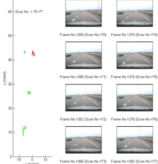
Figure 5 shows the object tracks on a highway using the probability-based segmentation. The maintenance tracks were plotted on the left and the corresponding video frames were shown on the right during eight scans. The green points and the red points represent the medium objects and the small objects, respectively. The rectangle points represent the points in the 77th scan and the number on the point is the track
ID. The security barriers were not tracked and the four tracks represent the four cars in front of the test vehicle. The car in the same lane was recognized as a small object because the laserscanner has a poor angular resolution to the far object. The track corresponding to the far car in the first lane (count from the left) was deleted in the 73th scan because of the
obscuration. Thus its track ID is not plotted in Fig. 5. Figure 6 shows the results of the complete object tracking algorithm when the test vehicle was driven on an urban street. The left column presents the results of the probability-based segmentation approach and the results using the distance -based segmentation approach were shown in the middle column. From the video frames in the right column we can see that only five vehicle-like objects need tracking and these vehicle-like objects were all tracked for both approaches. Although both distance-based and probability-based approaches generate tracks for non-vehicle-like objects along the road sides, it is clear from the simulation that the probability-based approach can effectively suppress these undesired tracks. The reduced number of dense tracks is
Figure 5. The maintenance tracks on a highway based on the probability-based segmentation during the eight scans (left) and the corresponding video frames (right).
beneficial to the computation load in the tracking step. This is because the possibility of a large number of joint association
events is reduced. A large number of joint association events
leads to heavier computational burden in tracking step. Figure 7 shows the tracking results using the probability-based segmentation approach when the test vehicle was driven on an urban street. The probability-based segmentation approach can also work well in the crowed environment most of the time.
VI. CONCLUSION
In this paper the probability-based segmentation approach was presented and the complete object tracking algorithm was simulated via the real traffic data. The results of the simulations show that the security barriers on a highway can be removed from the tracking step and the vehicle-like
Figure 6. The tracking results based on the probability-based segmentation approach (left) and the distance-based segmentation approach (middle) during the eight scans on a road and the corresponding video frames (right).
objects were tracked well. In addition, Dirichlet processes favor simpler models [5]. The small pieces of segment on the roadsides which are aligned roughly in the y/x direction are grouped in general except that the segment with long distance to that group. Therefore the probability-based segmentation approach can suppress the non-vehicle-like object tracks on the roadside because the segmentation result depends on the distribution of the observations instead of a threshold.
Figure 7. The tracking results based on the probability-based segmentation during the eight scans on a street (left) and the corresponding video frames (right).
REFERENCES
[1] K. Dietmayer, J. Sparbert, and D. Streller, “Model based object classification and object tracking in traffic scenes from range images,” IEEE Intelligent Vehicle Symposium, Tokyo, Japan, 2001.
[2] S. Santos, J. E. Faria, F. Soares, R. Araujo, and U. Nunes, “Tracking of multi-obstacles with laser range data for autonomous vehicles,” ROBOTICA 2003, Lisbon, Portugal, 2003.
[3] G. A. Borges and M.-J. Aldon, “Line extraction in 2D range images for mobile robotics,” Journal of Intelligent and Robotics Systems, vol. 40(3), pp. 267-297, 2004.
[4] D. Streller and K. C. Dietmayer, “Object tracking and classification using a multiple hypothesis approach”, IEEE Intelligent Vehicles Symposium, Parma, Italy, 2004.
[5] E. B. Fox, D. S. Choi, and A. S. Willsky, “Nonparametric Bayesian methods for large scale multi-target tracking,” Signal, system & Computers, ACSSC’06 Fortieth Asilomar Conference, pp. 2009-2013, Nov. 2006.
[6] D. Mušicki, R. Evans, and S. Stankovic, “Integrated probabilistic data association,” IEEE Transactions on Automatic Control, vol. 39(6), pp. 1237-1241, June 1994.
[7] D. Mušicki and R. Evans, “Joint Integrated Probabilistic Data Association - JIPDA,” IEEE Transaction on Aerospace Electronic Systems, vol. 40(3), pp. 1093-1099, July 2004.
[8] Y. W. Teh, M. I. Jordan, M. J. Beal, and D. M. Blei, “Hierarchical Dirichlet Processes,” Journal of the American Statistical Association, vol. 101(476), pp. 1566-1581, December 2006.
[9] R. M. Neal, “Markov chain sampling methods for Dirichlet process mixture models,” Journal of Computational and Graphical Statistics, vol. 9(2), pp. 249-265, June 2000.
[10] D. S. Caveney, “Multiple model techniques in automotive estimation and control,” PhD Dissertation, U. C. Berkeley, pp. 37-41, 2004. [11] Y. Bar-Shalom, X. R. Li, and T. Kirubarajan, “Estimation with