INTERNATIONAL JOURNAL FOR NUMERICAL METHODS IN ENGINEERING, VOL. 30, 1213-1228 (1990)
MINIMAX MULTIOBJECTIVE OPTIMIZATION IN
STRUCTURAL DESIGN
C. H. TSENG AND T. W. LU
Department of Mechanical Engineering, National Chiao Tung University, Hsinchu, Taiwan, 30050 R.0.C SUMMARY
The use of multiobjective optimization techniques, which may be regarded as a systematic sensitivity analysis, for the selection and modification of system parameters is presented. A minimax multiobjective optimization model for structural optimization is proposed. Three typical multiobjective optimization techniques-goal programming, compromise programming and the surrogate worth trade-off method-are used to solve such a problem. The application of multiobjective optimization techniques to the selection of system parameters and large scale structural design optimization problems is the main purpose of this paper.
INTRODUCTION
In most structural optimization problems, it is desirable that the structure should be of minimum weight and simultaneously meet some requirements such as strength, deflection and frequency. Usually, these requirements are imposed as inequality constraints, where the allowable strength, deflection and frequency are selected as fixed parameters in the problem formulation.' Parameter sensitivity analysis is thus needed if the requirements are modified after the optimization is complete. Interest toward this topic can be seen in the literature.'. It is noted that parameter analysis provides only a measure of changes of the optimum design within its neighbourhood. Another approach to treat the selection and modification of problem parameters is the use of multiobjective optimization techniques which may be regarded as a systematic sensitivity ana- l ~ s i s . ~
A general multiobjective optimization problem is to find the vector of design variables x = ( x ~ , x2,
. . . ,
x , ) ~ which minimizes a vector objective function f(x) = (fi(x),fi(x),. .
.
,A(x))~
over the feasible design spaceX.
It is the determination of a set of non-dominated solutions (or Pareto optimum solutions, non-inferior solutions or efficient solutions) that achieves a compro- mise among several different, usually conflicting, objective functions. The set of non-dominated solutions is a set of solutions in which no decrease can be obtained in any of the objectives without causing a simultaneous increase in at least one of the other objectives. The associated set of non-dominated objectives generally represents a collection of incomparable solutions for the objectives which are usually non-commensurable to begin with. Thus, here arises the decision making problem from which a partial or complete ordering of the set of non-dominated objectives is accomplished by considering the preferences of the decision maker (DM). Most of the multiobjective optimization techniques are based on how to elicit the preferences and determine the best-compromise solution.OO29-598 1/90/14 12 13-1 6$08.OO
0
1990 by John Wiley & Sons, Ltd.Received 8 August 1989 Revised 22 March 1990
1214 C. H. TSENG AND T. W. LU
In this paper, a general multiobjective optimization model for structural optimization is presented. The traditional minimum weight problem can be reformulated as a optimization problem with multiple minimax objectives to consider the significant design requirements simultaneously and be treated as the parameter selection problem. Multiobjective optimization methods available in the literature are mostly linear in n a t ~ r e . ~ Only a few non-linear methods are proposed with simple testing problems. The application of multiobjective optimization techniques to large scale problems is still rare. Three typical multiobjective optimization tech- niques, goal-programming, compromise programming and the surrogate worth trade-off method, are used to solve large scale structural systems with multiple minimax objectives. The determina- tion of system parameters by means of multiobjective optimization process is also discussed here.
PROBLEM FORMULATION
A common minimum weight structural optimization problem may be stated as the following. satisfy stress constraints
Find the design variables x =
(xl,
x2,.
. .
, x , ) ~ to minimize the weight of the structuref(x) and J a i l < a i a i = 1 , 2 ,. . . ,
n (1) lzjl<
zja (2) oi<
oF i = 1 , 2 , .. .
, n (3) 5 a<
t
(4) ( 5 ) displacement constraints j = 1 , 2 , .. . ,
r buckling constraintsfundamental frequency constraints
and design variable bounds
xi1
d
xi d Xi"where x can be the cross sectional area, length, width,
. . . ,
etc, of each member; cia and zja are the allowable stress for the i th member and allowable displacement for the j t h displacement component, respectively; qi is the stress in the ith member; z j is the j t h displacement component. The allowable buckling stress a! is obtained from the equation of the Euler critical load. 5, is the allowable eigenvalue calculated from the specified lower limit on the fundamental frequency. The fundamental frequency o can be calculated by solving the following eigenvalue problem:W ) Y
= 5M(X)Y (6)where M(x) is the r x r mass matrix, y is an eigenvector and
5
is an eigenvalue which equals w2.For detailed information of the derivation and calculation, references can be consulted in References 1 and 6.
Once the problem is formulated, a non-linear programming algorithm is exploited to perform the design optimization. But it should be noted that the specification of allowable parameters could be hard to select for the engineer. In fact, one may originally hope to minimize the weight and nodal displacements as well as member stresses and maximize the fundamental natural frequency simultaneously, which lead to a multiobjective optimization problem. All these objec- tives are non-commensurable and conflict in nature. From this point of view, it is desirable to relax the original single objective optimization problem to the multiobjective one.
MULTIMAX MULTIOBJECTIVE OPTIMIZATION 1215
Engineers and the decision makers will communicate to make a best-compromise design during the multiobjective optimization solution process. This would be beneficial to the balance among the specified objectives. As a result, we redefine the structural optimization problem as the following.
Find the design variable x which minimizes the weight of the structure, the maximum member stress and the maximum nodal displacement while the fundamental natural frequency is maxi- mized. Mathematically, it can be stated as
minf, (XI (7)
minf,(x) = max oi, i = 1,2,
. .
.
,
n (8) minf,(x) = max z j , j = 1,2,.
. .
, I (9)minf,(x) = - o (10)
subject to
Since the buckling strength of each member is o!, determined once the geometric property is given, the buckling constraint will not be treated as an objective here. With these objectives, one may be able to choose the system parameters by the solution of the multiobjective optimization problem, even for large scale ones. For example, a material with a strength greater than or equal to the maximum stress would be an appropriate selection for the structure. On the other hand, the maximum displacement should be reduced to fit the requirement of the performance of the structure. A higher fundamental frequency is preferred for the sake of vibration control. All the information obtained during the multiobjective optimization solution process is useful for the determination of allowable parameters of structural systems.
In the above general formulation, the selection of objectives depends on the DM and the engineer. Only those the DM considers worthwhile or whose performance is not certain to the engineer will appear in the set of objectives. Since most of the structural optimization problems in the real world are large scale ones, we have to deal with large scale structural optimization problems with multiple minimax objectives. Through the design of three structures, we attempt to show how multiobjective optimization techniques perform in the selection of system parameters as a systematic parameter sensitivity analysis and how they are adopted to solve large scale design problems.
SOLUTION PROCEDURES
A set of multiobjective optimization techniques which have been or may be applied to structural design problems was presented in References 4, 7 and 8. Generally, multiobjective optimization techniques can be classified into three categories according to the articulation of the decision maker's preference structure over the multiple objectives prior to, during or after the optimiza- tion. Based on this classification, an overall review of multiobjective optimization techniques and their applications is available in Reference 9. Three typical multiobjective optimization tech- niques-goal programming, compromise programming and the surrogate worth trade-off method-are thus chosen in this study, mainly because of their representative and thier promising features for future development in engineering design optimization.
1216 C. H. TSENG AND T. W. LU Goal programming
Goal programming, first presented in References 5 and 7, requires prior articulation of preferences by the DM. It allows the decision maker to specify a target for each objective function. A preferred solution is then defined as the one that minimizes the sum of the absolute values of deviations from the prescribed set of goal values.
A general formulation of goal programming for non-linear programming problems can be stated as follows:’o i = l subject to g,(x)
<
0, i = 1,2,.. .
, mhi@)
= 0, i = 1,2,. .
.
,
p J i ’ ( x ) - d : + d ; = T , i = l , 2, . . . ,
k d: 20, i = 1,2,. .
.
, k d ; 20, i = 1,2,. . . ,
kwhere
I;:
represents the target or goal set by the DM for the ith objective functionf,’(x) and d: and d ; are, respectively, the under-achievement and over-achievement of the ith objective and defined asNote that the value of p is based on the utility function chosen by the DM and it is possible to obtain non-dominated solutions by varying the values of p and
Ti.
Compromise programming
Compromise programming” is based on the concept of distance from an ideal solution, and the solutions which are closest to the ideal point are called compromise solutions and form the compromise set. When each objective functioni, i = 1,
. .
.
,
k, is characterized by ‘more is better’, one can set f * =(f:,
. . .
,f;),
where f f = sup($(x)lx EXI.
In this case, f* is called an ideal point because usually f*
is not attainable. Compromise was once remarked as the art of cutting the cake so that everyone thinks he or she got the largest piece. Here, compromise is considered as an effort to approach the ideal solution as closely as possible. The ideal solution, usually infeasible, is the situation where everybody does get the largest possible piece, though in compromise it is assumed that the cake is always smaller than the sum of claims on it.The generalized distance measure used in compromise programming to evaluate how close the set of non-dominated points come to the ideal point is the family of L, matrices defined as
X(x)
-
f:
llSLs =
{
-
ft
I
1
where 1
<
s<
co; ai are weights,ff a n d i m a x are the minimum value and the worst value for the ith objective respectively;f,(x) is the value of implementing the design variable x with respect toMULTIMAX MULTIOBJECTIVE OPTIMIZATION 1217
the ith objective. Therefore, the compromise programming model is formulated as follows: min L,(x) = L,(xf)
subject to x E
X
for a given set of weights cli and for all 1 6 s 6 co, where
X
denotes the feasible region.To find a compromise solution, one needs to know the ideal point f
*
=(f?,
. . .
, f f ) and the parameter s for the L,(x) matrices. For s = 1, all deviations fromff are taken into consideration in proportion to their magnitude. For 2<
s < 00, the larger the deviation, the larger the weightin L,. As s become larger and larger, and finally s = 00, the largest deviation is the only one taken
into account.
The surrogate worth trade-of method
The surrogate worth trade-off (SWT) method5’ 1 2 * l 3 is an interactive method, which can be
applied when design variables are continuous and objective functions and constraints are twice differentiable. It assumes that the preference of the decision maker is monotonic and can be exhibited as an implicit multiattribute utility function as the DM systematically compares two objectives at a time. The SWT method consists of three main steps. First of all, generate a representative subset of non-dominated solutions called ‘promising solutions’ and obtain the relevant trade-off information for each generated solution. Secondly, interact with the DM to elicit the preference (worth) structure. Finally, select the best-compromise solution from the information obtained.
Consider the E-constraint problem Pi(&)
min A ( x ) (18)
subject to $(x) 6 e j , j # i, j = 1,2,
. .
. ,k
X € Xwhere
X
is the original design space of the multiobjective optimization problem and E~ are knownas the maximum tolerable levels. It is used in the method to yield the promising solutions and associated trade-off information. By use of the concept of duality theory and Lagrange multipliers as well as the Kuhn-Tucker conditions, the trade-off function
Ti
can be defined asor
T.. = -
1..
V 1J
1,
is the generalized Lagrange multiplier associated with the ith E-constraint. More details of the derivation of the trade-off function can be seen in the Appendix and References 12 and 13. The trade-off ,Iij represents the marginal rate of substitution between the ith and j t h objectives. Note that only positive trade-offs are of interest here. Once the trade-offs have been identified, the decision maker is supplied with the trade-off information and then asked to express his ordinal preference. The DM’s preference is embodied in the surrogate worth function wij, which is ordinal and ranges from - 10 to+
10. It is an estimation of the desirability of the trade-off l i j . Thus,+
10 would indicate that 1, marginal units of the ith objective are very much more worthwhile than one marginal unit of thejth objective, while - 10 would indicate the opposite and 0 would signify an even trade. The best-compromise solution is determined when all trade-off ratios are selected to make the surrogate worth functions simultaneously equal to 0.1218 C. H. TSENG AND T. W. LU
Numerical implementation
Since the techniques for the single (scalar) objective optimization problem are well established, most multiobjective optimization techniques are based on transforming multiobjective problems into single objective ones in order to obtain the best-compromise solution by applying single objective optimization techniques directly. From the comparative studies of various single optimization algorithms available in the recent literat~re,'~-'* the mathematical programming method known as sequential quadratic programming (SQP) is selected in this paper for its accuracy, reliability and efficiency. The auxiliary single objective optimization problems needed during the solution process are solved by using the SQP algorithm in the optimization solver IDESIGN3.51. The IDESIGN3.51 program with a subroutine format is modified from IDESIGN3.5." It has been robustly implemented and extensively tested in a wide range of highly non-linear small and large scale problems for the SQP algorithm.20
One typical approach to a single minimax objective is the solution of the minimization of an introduced artificial variable which is the upper bound of the maximum value of the objective. For minimax multiobjective optimization problems, they can be treated along the way of the solution of a single objective problem to have more than one artificial variable. In the SWT method, for the trade-off interpretation in the minimax multiobjective problem one may refer to Chankong and Haimes.13
The ideal point is selected as the goal in goal programming. Since the ideal/worst point is the point at which each individual objective is minimized/maximized without regard to other objectives, the over-achievement constraint in equation (13) will be eliminated. But to find an ideal/worst point is not always attainable from the numerical point, which can be provided by the DM during the solution process. All the information of ideal and worst point for both goal and compromise programming may be calculated in the implemented program or given by the DM from input data.
For the analysis of the structures, the finite element method is used. And the necessary design sensitivity analysis is performed by the hybrid method,2' which combines the advantage of the direct differential method (DDM) and the adjoint variable method (AVM). The implementation of the three techniques is used for the solution of three large scale numerical design examples.
DESIGN EXAMPLES
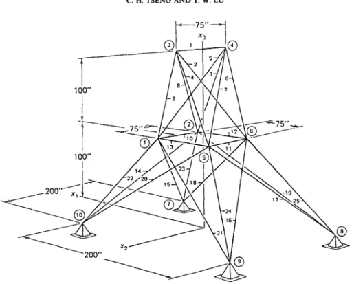
Three structural optimization problems frequently appearing in the literature are reformulated as multiobjective optimization problems, as discussed previously. They are, as shown in Figures 1-3, a ten-member cantilever truss, a twenty-five-member transmission tower and a two-hundred- member plane truss.' Three design problems are imposed, all constrained. The ten-member cantilever truss is solved with loading case 11. The twenty-five-member transmission tower design problem is considered under two loading conditions and the 200-bar truss is treated with three loading conditions. All the numerical data are the same as those in Reference 1, while the allowable parameters are abandoned and will be determined during the multiobjective optimiza- tion solution (decision making) process.
Tables I-V shows the best-compromise solutions and trade-off information for the three example problems. Note that the ideal value and worst value of maximum stress, displacement and minus frequency are provided by the DM or the engineer. The range between the ideal and worst values may be associated with the properties of available materials or requirements of the design. Trade-offs between the objectives prior to, during or after the solution process are
M ULTIMAX MULTIOBJECTIVE OPTIMIZATION
-
XIFigure 1. Ten-member cantilever truss
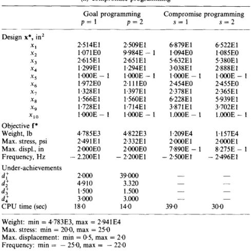
Table I. Results for the ten-member cantilever truss by (i) goal programming;
(ii) compromise programming Goal programming p = l p = 2 Compromise programming s = l s = 2 Design x*, in2 X i x2 x3 x4 x5 x7 X8 x 9 X I 0 Objective f* Weight, Ib Max. stress, psi Max. displ., in Frequency, Hz Under-achievements x6 d: d: d: d:
CPU time (sec)
2.514E1 1.071EO 2-615E1 1.299E1 1.972E0 1.328E1 1.566E1 1.728E1 1.000E - 1 1WOE - 1 4.785E3 2.49 1 E 1 2900EO - 2.200E1 24300 4.910 1.500 3.000 18.0 2.509E1 9.984E - 1 2-65 1El 1.294E 1 2.1 11EO 1.397E1 1.560E1 1.714E 1 1OOOE - 1 1OOOE - 1 4.822E3 2.332E1 2.000EO - 2’200E1 39.000 3.320 1.500 3.000 14.0 6.879E1 1.094EO 5632E1 3.038E1 2.454EO 2.378E1 6.228El 3.871 E 1 1OOOE - 1 1.000E - 1 1.209 E4 2.000E 1 7’890E - 1
-
2‘500E1 - - - - 39.0 6.522E1 1.085EO 5.380E1 2.888E1 2.455E0 2.365E1 5.939E1 3.702E1 1.000E - 1 1.000E - 1 1.157E4 2WOE 1 8.275E - 1 - 2.496El - - - - 30.0 1219Weight: min = 4.783E3, max = 2.941E4
Max. stress: rnin = 20.0, max = 25-0
Max. displacement: min = 0.5, max = 2.0
1220 C. H. TSENG AND T. W. LU
Figure 2. Twenty-five-member transmission tower
Table 11. Trade-off information and the best-compromise solution for the ten-member cantilever truss design problem by the SWT method assuming the existence of a decision maker
f,
h
f, f, 4 2 1 1 3 '$4 w12 w13 w14Ideal value: Worst value:
4.783E3 200 0.5 - 25-0
2.941 E4 25.0 2.0 - 22.0 Referenced objective: Weight
( A
)Maximum tolerable levels: Trade-off
22.5 1-2 - 23.0
1 9.98E3 2'15E1 9'20E - 1 - 2.38E1 1'17E2 9.66E3 4.89E3 0
+
3 - 22 9.34E3 215E1 9.90E - 1 - 2'40E1 1-3382 8'99E3 5'09E3 0 0
+
2 3 9.32E3 2.15E1 9'90E - 1 - 2.39E1 1'28E2 8.99E3 4.87E3 0 0 0Objectives
Best-compromise solution
f,
h
f,9.3 192E3 2.1500E1 9'9000E - 1 - f 4 2.3900E1 Designs
1 2 3 4 5 6 7 8 9 10
55.775 1.147 4.964 2.420 0.1 2.279 18.447 38.470 31.887 0.1 CPU time (sec) 55.0
MULTIMAX MULTIOBJECTIVE OPTIMIZATION
4-240"+
1221
accomplished by communication of the DM or the engineer to the program. Resources and constraints affect the solution process largely. For example, materials available for the design should be taken into consideration when the trade-off between maximum stress and other objectives proceeds. Maximum displacement directly affects the performance of the structure. And weight represents the cost, while fundamental frequency is important for excitation vibra- tion. All these objectives are non-commensurable and may conflict with each other. After the
1222 C. H. TSENG AND T. W. LU
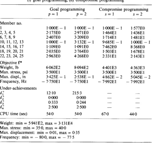
Table 111. Results for the twenty-five-member transmission tower design problem by (i) goal programming; (ii) compromise programming
Goal programming p = l p = 2 Compromise programming s = l s = 2 Member no. 1 2, 3, 4, 5 6, 7, 8, 9 10, 11, 12, 13 14, 15, 16, 17 18, 19, 20, 21 22, 23, 24, 25 Objective f* Weight, lb Max. stress, psi Max. displ., in Frequency, Hz Under-achievements d :
a,+
a:
a,'
CPU time (sec)
1WOE - 1 2.175EO 2.407E0 1.109EO 2.035E0 2.963E0 19OOE - 1 6.062E2 3.500E1 3.425E - 1 - 7.750E1 12.10 0.OOO 0333 2.500 54.0 1WOE - 1 2.971E0 3.209E0 1.09 1 EO 2.764E0 4.268E0 3.132E - 1 8.094E2 3.500El 2.538E - 1
-
7.750E1 215.3 0.000 0.244 2.500 54.0 1QOOE - 1 1.577E0 1.464E1 1.436E1 1.714E1 1.48 1 E 1 7.462E0 8.368EO 1.503E1 1.678E1 2.33 1El 2.143E1 9.685E - 1 1'000E - 1 4.40 1 E3 4.363E3 3.500E1 3.500E1 4'862E - 2 5.0458 - 2 - 7'992El - 7.992E1 67.0 44.0Weight: min = 5.941E2, max = 3.131E4 Max. stress: min = 35.0, max = 40.0 Max. displacement: min = 0.01, max = 0.35 Frequency: min = - 80.0, max = - 77.5
best-compromise solution is reached, system parameters can be determined according to the solution. It is noted that design alternatives are compared systematically during the solution process while traditional parameter sensitivity analysis yields only local information after the optimization.
Goal programming gives maximum values for maximum displacement and frequency objec- tives with p = 1 and p = 2 in 10-bar truss design problem, as shown in Table I. Frequency objective achieves the worst point for all the cases except p = 1 in 200-bar case. In the 25- and 200-bar truss design problems, the maximum stress equals the ideal value. All this information is clear with the investigation of under-achievements. It should be noted that a solution is a dominated solution if the under-achievements are all zero.
The last row of the tables shows the CPU time needed on Apollo D N 570. Evidently the 200-bar truss design case requires much CPU time. Generally, compromise programming requires more CPU time than goal programming does. It produces higher weight and lower maximum displacement for all the cases. This is the scaling and weighting effect, both of weight and maximum displacement.
For goal and compromise programming, the ideal point is selected as the goal. However, the DM may choose his favourite point as his goal and the balance between the objectives may be in terms of the value of p and s or the weightings a. So the best-compromise solution would be different for other DMs. This can be seen in the solution process of the SWT method.
MULTIMAX MULTIOBJECTIVE OPTIMIZATION 1223
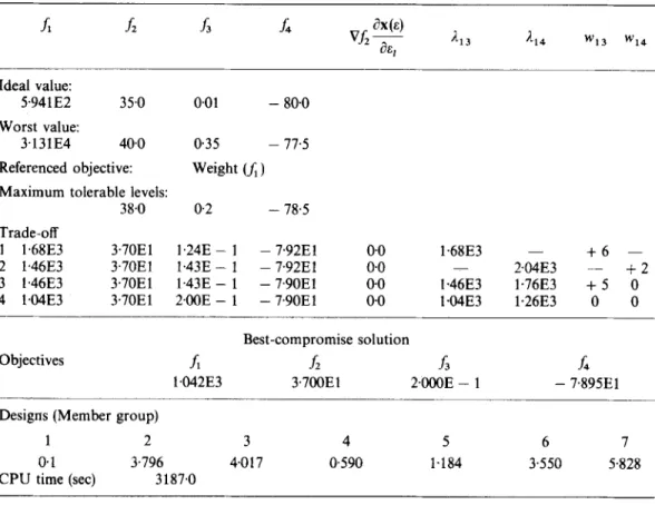
Table IV. Trade-off information and the best-compromise solution for the twenty-five-member trans- mission tower design problem by the SWT method assuming the existence of a decision maker
Ideal value: Worst value:
Referenced objective: Weight
ul
)Maximum tolerable levels: Trade-off
1 1.68E3 3.70E1 1.24E - 1 - 7.92E1 0.0 1.68E3 + 6 -
2 1.46E3 3.70E1 1'43E - 1 - 7.92E1 0-0 2-04E3 - + 2
3 1.46E3 3'70E1 1'43E - 1 - 7'90E1 0.0 1.46E3 1.76E3
+ 5
0 4 104E3 3'70E1 200E - 1 - 7'90E1 0.0 l94E3 1.26E3 0 05.94 1 E2 3 5.0 0.01 - 80.0 3.1 3 1 E4 40.0 0.35 - 77.5 38.0 0.2 - 78.5 - - Objectives Best-compromise solution f, f, f,
h
1W2E3 3.700E1 2.000E - 1 - 7'895E1 Designs (Member group)
1 2 3 4 5 6 7
0.1 3.796 4.01 7 0590 1.184 3-550 5.828
CPU time (sec) 3187.0
Table V. Results for the two-hundred-member plane truss design problem by (i) goal programming; (ii) compromise programming
Objective f
*
Weight, lb Max. stress, psi Max. displ., in Frequency, Hz Under-achievementsCPU time (sec)
Goal programming Compromise programming
p = l p = 2 s = l s = 2 2.94 1 E4 2.500E1 5.000E - 1 - 5'000EO O.Oo0 O W 0 0.456 5.OOo 20 825.0 3.580E4 2.500E1 4.267E - 1 - 6.444E0 0.639E4 O~OOO 0.382 3.556 17 259.0 1.518E5 2.500E1 1.415E
-
1 - 1OOE1 37 342.0 1-582E5 2.500E1 1.3938 - 1 - 9.745E0 20 361.0 Weight: rnin = 2.941E4, max = 6-578E5Max. stress: min = 25.0, max = 30.0 Max. displacement: min = 0.0445, max = 0.5 Frequency: min = - 10.0, max = - 5.0
1224 C. H. TSENG AND T. W. LU
Recall that we are dealing with positive Lagrange multipliers as the trade-offs. It is necessary to treat zero trade-offs Lij because of the improper selection of cj or the non-conflicting nature between the j t h objective and the referenced objective. The situation may occur if there are several objectives. In the solution of 25- and 200-bar design problems, we have encountered such a case. It is noted that the given cj for the &-constraint of the stress objective may not produce a positive trade-off rate because of the limitation of buckling constraints and the interaction with other objectives. To handle such zero
Liis,
we have to ask the DM the following question: 'How would you like to decreasef, byA:,
units and change6 by V ~ ( X ' ) * dx(c')/dc, units, while increasingf; byone unit? Given that
fj
= 6 ( x i )
for all j = 1,. .
.
,
n.'Note that determining dx(~')/ds, is not easy for large scale problems, especially for structural optimization problems. This may be the main difficulty we have to overcome. Here in this section we use forward difference to compute ~ X ( E ~ ) / ~ E , as
dX(&i) X(Ef) - x i
d E l 8%
x
where cf = (ci, E : ,
. . . ,
cf+
BE,, . . . ,
EL-
As a result, we have to solve more auxiliary singleobjective optimization problems each time before the above question is asked, depending on the number of positive &'s. Moreover, the trade-off rate between minimax objectives should be noted.
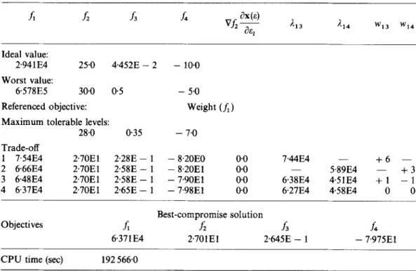
Tables 11, IV and VI display the summary of the trade-off information and the best-compro- mise solution obtained by the SWT method. From these results, we may realize that trade-offs of weight to maximum displacement and frequency are much more significant than to the maximum
Table VI. Trade-off information and the best-compromise solution for the two-hundred-member plane truss design problem by the SWT method assuming the existence of a decision maker
f ,
"6
f,Ideal value: Worst value: Referenced objective: Maximum tolerable levels: Trade-off
2.941E4 25.0 4.452E - 2 6578E5 3 0 0 0 5
28.0 0 3 5
1 7.54E4 270E1 2 2 8 E - 1
2 6.66E4 2'70E1 2'58E - 1 3 6.48E4 2'70E1 2.58E - 1 4 6.37E4 2'70E1 2.65E
-
1- 10.0
- 7.0
-
- 8'20EO 0 0 7.44E4 + 6 -
- 8'20E1 0.0 5.89E4 - + 3
- 7*90E1 0.0 6.38E4 4.51E4
+
1 - 16.27E4 458E4 0 0 - 7.98El 0 0 - Objectives Best-compromise solution
A
"6
f, f,6.371E4 2.70 1 E 1 2.645E - 1 - 7'975E1
S E L E C T T H E REFERENCE OBJECTIVE : (1.4) 1
PROVIDE THE MAXIMUM TOLERABLE LEVEL OF OBJECTIVE 2 : ( 2.500E+01, 3.000E+01) 28.0
PROVIDE THE MAXIMUM TOLERABLE LEVEL OF OBJECTIVE 3 : ( 4.4523-02, 5.OOOE-01) 0.35
PROVIDE THE MAXIMUM TOLERABLE LEVEL OF OBJECTIVE 4 :(-1.000E+01,-5.000E+OO) -7.0
TOLERA8LE LEVEL OF OBJECTIVE 2 USED IS 2.800000000E+01 TOLERABLE LEVEL OF OBJECTIVE 3 USED IS 2.2780705203-01 TOLERABLE LEVEL OF OBJECTIVE 4 USED IS -8.200000000E+00 *****THE SUBPROBLEM IS FEASIBLE*****
HOW MUCH WOULD YOU LIKE TO DECREASE F1 BY 7.4423+04 UNITS AND CHANGE F2 BY O.OOE+OO UNITS WHILE INCREASING F3 BY ONE UNIT ? GIVEN THAT :
OBJECTIVE 1: 7.5373+04 2: 2.701E+01 3: 2.2783-01 4:-8.2003+00 PLEASE PROVIDE YOUR SURROGATE WORTH : (10,-lo)?
6
TOLERABLE LEVEL OF OBJECTIVE 3 USED IS 2.5835301093-01
HOW MUCH WOULD YOU LIKE TO DECREASE F1 BY 5.8873+04 UNITS AND CHANGE F2 BY O.OOE+OO UNITS WHILE INCREASING F4 BY ONE UNIT ? GIVEN THAT :
OBJECTIVE 1: 6.6573+04 2: 2.701E+01 3: 2.5843-01 4:-8.200E+00 PLEASE PROVIDE YOUR SURROGATE WORTH : (10,-lo)?
3
TOLERABLE LEVEL OF OBJECTIVE 4 USED IS -7.899918000E+00 *****THE SUBPROBLEM IS FEASIBLE*****
HOW MUCH WOULD YOU LIKE TO DECREASE F1 BY 6.3833+04 UNITS AND CHANGE F2 BY O.OOE+OO UNITS WHILE INCREASING F3 BY ONE UNIT ? GIVEN THAT :
OBJECTIVE 1: 6.4763+04 2: 2.701E+01 3: 2.5843-01 4:-7.9003+00 PLEASE PROVIDE YOUR SURROGATE WORTH : (10,-lo)?
1
HOW MUCH WOULD YOU LIKE TO DECREASE F1 BY 4.5103+04 UNITS AND CHANGE F2 BY O.OOE+OO UNITS WHILE INCREASING F4 BY ONE UNIT ? GIVEN THAT :
OBJECTIVE 1: 6.4763+04 2: 2.701E+01 3: 2.584E-01 4:-7.900E+00 PLEASE PROVIDE YOUR SURROGATE WORTH : (10,-lo)?
-1
TOLERABLE LEVEL OF OBJECTIVE 2 USED IS 2.800000000E+01 TOLERABLE LEVEL OF OBJECTIVE 3 USED IS 2.6446220273-01 TOLERABLE LEVEL OF OBJECTIVE 4 USED IS -7.974930500E+OO
HOW MUCH W O U L D YOU LIKE T O DECREASE F1 BY 6.274Et04 UNITS AND C H A N G E F2 BY 0.000Et00 UNITS WHILE INCREASING F 3 BY O N E UNIT ? G I V E N T H A T :
OBJECTIVE 1: 6.371Et04 2: 2.701Et01 3: 2:645E-01 4:-7.975EtOO P L E A S E P R O V I D E YOUR SURROGATE W O R T H : (10,-10)?
0
HOW MUCH WOULD YOU LIKE TO DECREASE F1 BY 4.580E+04 UNITS AND CHANGE F2 BY O.OOOE+OO UNITS WHILE INCREASING F4 BY ONE UNIT ? GIVEN THAT :
OBJECTIVE 1: 6.3713+04 2: 2.701E+01 3: 2.645E-01 4:--7.9753+00 PLEASE PROVIDE YOUR SURROGATE WORTH : (10,-lo)?
0
*****REACH THE BEST-COMPROMISE SOLUTION*****
Figure 4. An illustration of the interactive solution process for the optimization of structures with multiple minimax objectives by the SWT method assuming the existence of a decision maker (200-bar case)
1226 C. H. TSENG AND T. W. LU
stress. This agrees with those obtained by goal and compromise programming methods. Figure 4 is an illustration of the interactive solution process for the optimization of structures with multiple minimax objectives. During the interactive process, the D M or the engineer can systematically compare the objectives from the trade-off information provided by the program and reach the best-compromise solution.
CONCLUSION
The use of a minimax multiobjective optimization model to provide a systematic parameter sensitivity analysis is discussed. Three structural optimization problems are reformulated and solved by three multiobjective optimization techniques. Among these methods, goal and compro- mise programming need less computational effort but the trade-off between objectives is much difficult than for the SWT method. This is because the SWT method uses first order information of the objectives. If the D M or the engineer has already had a favourite goal in mind, goal programming may be used. On the other hand, compromise programming will be chosen if the computational efforts are emphasized and the specific goal is not provided in advance. The SWT method gives a very good procedure for the systematic parameter sensitivity analysis though it requires much more computational effort. Numerical experience of the SWT method shows that the optimum point for each auxiliary single objective optimization problem may be taken as the initial guess for the next one. Such a treatment may significantly save computational effort.
The selection of the system parameters before the optimization is difficult. It is even more difficult for large scale problems. This paper solved the problem and completed the application of multiobjective optimization techniques to large scale structural design optimization problems.
ACKNOWLEDGEMENT
The research reported in this paper is supported under a project sponsored by the National Science Council Grand, Taiwan, R.O.C., NSC78-0401-E009-12.
APPENDIX
Trade-ofS functions
For the multiobjective optimization problem formulated as min J i ( X ) , i = 1,2,
. . .
, k&(X) d 0, i = 1,2,
. . .
, m subject tothe trade-off function, denoted
T j ( x ) ,
between the ith and j t h objectives, is defined aswhere
It is evident that the direct use of the definition is impractical and prohibitive. Thus, the concept of duality theory and Lagrange multipliers in non-linear programming as well as the &-constraint method are used as the alternative approach to construct the trade-off matrix.
MULTIMAX MULTIOBJECTIVE OPTIMIZATION 1227
The &-constraint problem Pi(&) can be considered as
minX(x) (A41
subject to
f ; . ( x ) < ~ ~ , j # i , j = l , 2
, . . . , k
gl(x)
<
0, 1 = 1,2,.
.
.
, rn (A6) where ej = f j * ( x )+
&>, j # i, j = 1,2,. . . ,
k, 2 0,j # i, j = 1,2,. . .
, k.f*(x) are the minimumsolution of the ith objective of problem ( A l ) and E; will be varied parametrically in the process of
constructing the trade-off functions. c j are known as the maximum tolerable levels. The gener- alized Lagrangian L of problem (A4) is
?n k
where p k and
lij
are the generalized Lagrange multipliers. The behaviour of the minimum value of the objective function as E~ varies is of special interest, so we haveor
aL
aEj
‘..
=-
-Applying the Kuhn-Tucker conditions,
Aij 2 0, Aij(fi(x) - e j ) = 0, j # i, i, j = 1,2,
. . .
, k (‘410)p L r > O , p l g l = O , Z = l , 2
, . . . ,
m (A1 1) andfi’(x) = L.We find that equations (AlO)-(All) hold only if
A,
= 0, or fj(x) - e j = 0, or both. Only non-zero Lagrange multipliers correspond to the non-dominated solutions, whereas the zero Lagrange multipliers correspond to the dominated solutions. It should be noted that only those Lij > 0, which impliesJ(x) = E ~ , are important for our analysis. Therefore, equation (A9) becomesor
T.. = -
1..
1J 1J
There exist the following relationships between 1,:
l k j = l k i A i j for all k # j 6414) and
1
’ k i =
1228 C. H. TSENG AND T. W. LU 1. 2. 3. 4. 5. 6. 7. 8. 9. 10. 11. 12. 13. 14. 15. 16. 17. 18. 19. 20. 21. REFERENCES
E. J. Haug and J. S. Arora, Applied Optimal Design: Mechanical and Structural Systems, Wiley, New York, 1979. G. N. Vanderplaats and N. Yoshida, ‘Efficient calculation of optimum design sensitivity’, AIAA J., 23, 1798-1803
(1985).
T. J. Beltracchi and G. A. Gabriele, ‘A RQP based method for estimating parameter sensitivity derivatives’, The 1988 ASME Design Technology Conferences-The Design Automation Conference, D E - VOL. 14, ASME, New York, 1988, J. Koski, ‘Multicriterion optimization in structural design’, in E. Atrek et al. (eds.), New Directions in Structural Design, Wiley, New York, 1984.
A. Goicoechea, D. R. Hansen and L. Duckstein, Multiobjective Decision Analysis with Engineering and Business Applications, Wiley, New York, 1982.
J. S. Arora, ‘On improving efficiency of an algorithm for structural optimization and a user’s manual for program trussopt3’, Technical Report No. 12, Materials Engineering Division, The University of Iowa, Iowa City, IA 52242,
1976.
L. Duckstein, ‘Multiobjective optimization in structural design: The model choice problem’, in E. Atrek et al. (eds.), New Direc-tions in Optimum Structural Design, Wiley, New York, 1984.
J. Koski and R. Silvennoinen, ‘Pareto optima of isostatic trusses’, Comp. Methods Appl. Mech. Eng., 31, 265-279 (1 982).
C. H. Tseng and T. W. Lu, ‘Multiobjective optimization in mechanical and structural design’, Math. Comp., submitted. S . S . Rao, V. B. Venkayya and N. S. Khot, ‘Optimization of actively controlled structures using goal programming techniques’, Int. j . numer. methods eng., 26, 183-197 (1988).
M. Zeleny, Multiple Criteria Decision Making, McGraw-Hill, New York, 1982.
Y. Y. Haimes and W. A. Hall, ‘Multiobjectives in water resource systems analysis: The surrogate worth trade OK
method‘, Water Resources Rex, 10, 615424 (1974).
V. Chankong and Y. Y. Haimes, Multiobjective Decision Making: Theory and Methodology, North-Holland,
Amsterdam, 1983.
E. Sandgren and K. M. Ragsdell, ‘The utility of nonlinear programming algorithms: A comparative study-Part I and
II’, J. Mech. Des., 102, 54&551 (1980).
W. Hock and K. Schittkowski, ‘A comparative performance evaluation of 27 nonlinear programming codes’,
Computing 30, Springer-Verlag, Berlin, 1983, pp. 335-358.
A. D. Belegundu and J. S. Arora, ‘A study of mathematical programming methods for structural optimization, Part I:
Theory, Part 11: Numerical aspects’, Int. j . numer. merhods eng., 21, 1583-1624 (1985).
P. B. Thanedar, J. S. Arora, C. H. Tseng, 0. K. Lim and G. J. Park, ‘Performance of some SQP algorithms on structural design problems’, Int. j . numer. methods eng., 23, 2187-2203 (1986).
C. H. Tseng, J. J. Tsay, 0. K. Lim, G. J. Park and J. S. Arora, ‘Performance of several optimization algorithms on a set of nonlinear programming test problems’, Technical Report No. ODL-87.2, Optimal Design Laboratory, College of Engineering, The University of Iowa, Iowa City, IA 52242, 1987.
C. H. Tseng and J. S. Arora, ‘On implementation of computational algorithms for optimal, design 1: Preliminary investigation, design 2 Extensive numerical investigation’, Int. j. numer. methods eng., 26, 1365-1402 (1988).
I. S. Arora and C. H. Tseng, ‘IDESIGN user’s manual version3.5’, Technical Report No. ODL-87.1, Optimal Design Laboratory, College of Engineering, The University of Iowa, Iowa City, IA 52242, 1987.
C. H. Tseng and K. Y. Kao, ‘Performance of a hybrid design sensitivity analysis on structural design problems’, Comp. Struct., 33, 1125-1131 (1989).