多維度的細胞分化在數學上的研究

國 立 交 通 大 學

應用數學系

碩

士

論

文

多維度的細胞分化在數學上的研究

Mathematical Studies on Multi-dimensional

Cellular Differentiation Models

研 究 生：劉兆涵

指導老師：石至文 教授

多維度的細胞分化在數學上的研究

Mathematical Studies on Multi-dimensional Cellular

Differentiation Models

研 究 生：劉兆涵 Student：Chao-Han Liu

指導教授：石至文 Advisor：Chih-Wen Shih

國 立 交 通 大 學

應 用 數 學 系

碩 士 論 文

Submitted to Department of Applied Mathematics College of Science

National Chiao Tung University in Partial Fulfillment of the Requirements

for the Degree of Master

in

Applied Mathematics December 2008

Hsinchu, Taiwan, Republic of China

多維度的細胞分化在數學上的研究

學生：劉兆涵 指導老師：石至文 教授

國立交通大學應用數學系(研究所)碩士班

摘 要

我們分析並總結在文獻裡提到的三個細胞分化模型的數學特

性。這些數學模型描述細胞分化過程中ㄧ些相關蛋白質與基因表現控

制網路中多重開關之動態。這些系統是可由多個對抗性分部所組成，

在基因控制中，每一分部各以全有或無之方式引導細胞分化成特定之

形式。

Mathematical Studies on Multi-dimensional

Cellular Differentiation Models

Student : Chao-Han Liu

Advisor : Chih-Wen Shih

Department of Applied Mathematics

National Chiao Tung University

Hsinchu, Taiwan, R.O.C.

December 2008

We summarize mathematical properties for three cellular differentiation models proposed in the literatures. These mathematical models are used to describe basic multi-switching dynamics in generic master regulatory net-works. These systems consist of arbitrary number of antagonistic components which direct differentiation in an all-or-none fashion to a specific cell-type chosen in gene regulation.

誌 謝

在這三年的研究生涯中，我要感謝的人很多。首先感謝我的指導

教授，因為我這個學期在高中做教育實習的工作，所以平日無法與老

師進行討論，很感謝老師挪出很多次的星期日傍晚時間與我進行論文

細部的討論，在論文架構初步完成後，就要進行文章的撰寫，這時我

從老師身上學到數學文章的表達，這段時間的訓練，真的要非常感謝

我的指導教授，對我將來在處事上必定有所幫助。

接下來，我要感謝口試委員，在口試時給我的建議，讓我更加瞭

解數學的嚴謹性。同時也要感謝教導過我的老師們，因為在每一門課

程都是在累積我的數學知識。

林光暉學長和廖康伶學姐是我要特別感謝的學長姐，謝謝你們在

我無助的時候給我打氣加油，在我開心時陪我一起歡笑。其他的學長

姐和同學們，也謝謝你們給我支持，讓我可以堅持下去。

最後，我要感謝我的家人，在我低潮時陪我度過難關，不讓我有

太大的壓力，此份榮耀，我要與你們分享。

Contents

1 Introduction 1

2 Model with mutual inhibition and autocatalysis 3 3 Model with mutual inhibition, autocatalysis, and leak 11

1

Introduction

Cellular differentiation is the process by which a less specialized cell becomes a more specialized cell type. Differentiation occurs numerous times during the development of a multicellular organism as the organism changes from a single zygote to a complex system of tissues and cell types. How the differentiation proceeds is the context of gene regulation and is rather complex. Several mathematical models have been proposed to depict and analyze the process. There were some reports on bistable switches for systems with two variables, for example, in [3], [7]. From experimental evidence, switching involving more than two variables and outcomes also deserves investigations.

In this report, we study three models proposed by Olivier and Demongeot [4]. The model consists of arbitrary number of components. Each of them represents the intracellular concentration of a differentiation factor, called switch element. Each of these components promotes itself and represses all others. Each of these variables can be regarded as a protein which corresponds to an antagonistic factor in the cell differentiation, for example, in hematopoiesis. These models aim at characterizing multi-dimensional switches in the cellular differentiation. In particular, the phases of co-expressed components and some up-regulating, some down-regulating are desired dynamic features in the models.

In the following, we discuss the properties of these models. The presentation is organized as follow. Section 2 addresses the model with mutual inhibition and autocatalysis. Each switch element is supposed to undergo non-regulated degra-dation (modelled as exponential decay, with an arbitrary speed 1), and transcrip-tion/translation with a relative speed σ. Each element positively auto-regulates itself, and represses expression of others, with a cooperativity c. Calling xi the

concentration of each switch element, the corresponding equations are

˙ xi = −xi+ σxc i 1 +Pn_j=1xc j , 1 ≤ i ≤ n.

Section 3 addresses the model with mutual inhibition, autocatalysis and leak. The model is the same as previously, except that each element has a ”leaky” ex-pression, modelled as a constant production term α. The equations become

˙ xi = −xi+ σx c i 1 +Pn_j=1xc j + α, 1 ≤ i ≤ n.

Section 4 addresses a model for bHLH proteins. Each switch bHLH protein is supposed to bind to a common activator according to the law of mass action, with a binding constant Kc, and a total quantity of activator at.

˙ xi = −xi+ σ( atxi 1+Pnj=1xj) c Kc+ (₁₊Patnxi j=1xj) c, 1 ≤ i ≤ n.

Throughout the presentation, we consider the system on the cone {(x1, x2, · · · , xn) : xj ≥ 0, j = 1, 2, · · · , n},

and we consider the following five kinds of equilibria for the three model systems: (i) the origin

(0, 0, · · · , 0) ∈ Rn_{; (1.1)}

(ii) One switch on and (n−1) off, i.e., the equilibrium (¯x1, ¯x2, · · · , ¯xn) with ¯xi = a 6=

0 for some i ∈ {1, 2, · · · , n} and ¯xj = 0 for all others j. Without loss of generality,

we set it as

(a, 0, 0, · · · , 0) ∈ Rn_{; (1.2)}

(iii) k switches on with identical components (k > 1), and (n − k) off (zero), i.e., the equilibrium (¯x1, ¯x2, · · · , ¯xn) with k’s i ∈ {1, 2, · · · , n} such that ¯xi = a 6= 0 and

¯

xj = 0 for all others j. Without loss of generality, we set it as

(a, a, · · · , a, 0, 0, · · · , 0) ∈ Rn_{; (1.3)}

(iv) all switches on with identical components, i.e., the equilibrium (¯x1, ¯x2, · · · , ¯xn)

with ¯xi = a 6= 0 for all i ∈ {1, 2, · · · , n},

(a, a, · · · , a) ∈ Rn_{; (1.4)}

(v) k switches on with identical components, and (n − k) off with identical com-ponents, i.e., the equilibrium (¯x1, ¯x2, · · · , ¯xn) with k’s ¯xi = a 6= 0, and (n − k)’s

¯

xj = b 6= 0 for i, j ∈ {1, 2, · · · , n} where k > 1 and (n − k) > 1 and a > b. Without

loss of generality, we set it as

(a, a, · · · , a, b, b, · · · , b) ∈ Rn_{. (1.5)}

We shall analyze the existence of those equilibria. In addition, we study the stability of these equilibria through linearization at these equilibria; namely, if all

eigenvalues have negative real parts, then the equilibrium is stable; if one of the eigenvalues has positive real part, then the equilibrium is unstable. As the first two models are gradient systems, we also justify that the global convergence for these systems.

In this report, propositions 2.1, 3.1, 3.2, 3.4, and 3.5 are completed in this study, while the others are recasted from [4], with more details.

2

Model with mutual inhibition and autocatalysis

In the section, we consider the equations ˙ xi = −xi+ σxc i 1 +Pn_j=1xc j , 1 ≤ i ≤ n (2.1)

where xi > 0 is the concentration of each switch element, σ > 1 is transcription/

translation with a relative speed, and c is cooperativity. Clearly, the origin is an equilibrium for every c > 0. In addition, if c ≥ 1, then the i-component of an equilibrium is either zero or satisfies

σxc−1_i

1+Pnj=1xcj = 1

⇔ 1 +Pn_j=1xc

j = σxc−1i .

Next, we consider three cases for c, i.e. c = 0, c = 1, and c > 1. If c = 0, then (2.1) becomes

˙

xi = −xi+

σ

1 + n, 1 ≤ i ≤ n. Let the right hand side of (2.1) be fi, Jij = ∂fi/∂xj. Then

Ji,i = −1 + (1 +Pn_j6=ixc j)(σcxc−1i ) (1 +Pn_j=1xc j)2 , (2.2) Ji,j = −σcxc ixc−1j (1 +Pn_j=1xc j)2 for j 6= i.

Proposition 2.1. For c = 0, there exists a stable equilibrium with all switches on, whose components are identically σ/(1 + n).

Proof: Consider the existence of the equilibrium with all switches on, whose com-ponents are identical. We have (σ/(1 + n), σ/(1 + n), · · · , σ/(1 + n)) ∈ Rn _{is an}

equilibrium. Next, consider the local stability of the equilibrium. Note that the linearization at (σ/(1 + n), σ/(1 + n), · · · , σ/(1 + n)) is      −1 0 · · · 0 0 −1 ... ... ... ··· ... 0 0 · · · 0 −1     .

We have all eigenvalues are negative. Thus, the equilibrium is stable. The assertion follows.

Example 2.1: In proposition 2.1, if n = 2 and σ = 2, i.e., the system is ½

˙

x1 = −x1 +₁₊₂2

˙

x2 = −x2 +₁₊₂2 ,

then (2/3, 2/3) is a stable equilibrium for the above system (see figure 1).

0 0.2 0.4 0.6 0.8 1 1.2 1.4 1.6 0 0.2 0.4 0.6 0.8 1 1.2 1.4 1.6

Figure 1: (2/3, 2/3) is a stable equilibrium (in example 2.1).

Next, consider c = 1 (no cooperativity), then (2.1) becomes ˙

xi = −xi+

σxi

1 +Pn_j=1xj

, 1 ≤ i ≤ n.

Suppose σ > 1. If xi 6= 0 for some i, then 1 +

P_n

j=1xj = σ. Note that the set

{(x1, x2, · · · , xn)|1 + n

X

j=1

is a hyperplane of equilibria. In addition, (2.2) becomes Ji,i = −1 + σ(1 +Pn_j6=ixj) (1 +Pn_j=1xj)2 , (2.4) Ji,j = −σxi (1 +Pn_j=1xj)2 for j 6= i.

The result of proposition 2.2. is only stated in [4]. We provide a detailed proof herein.

Proposition 2.2. ([4]) For c = 1 and σ > 1, the hyperplane of equilibria (2.3) is stable and the origin is an unstable equilibrium.

Proof: With (2.4), the origin is unstable since −1 + σ > 0 is the only eigenvalue. Consider the distance from the point (x1(t), x2(t), · · · , xn(t)) to the hyperplane

y1+ y2+ · · · + yn = σ − 1.

Set the square of distance of a point (x1, x2, · · · , xn) to the plane as

D(x1, x2, · · · , xn) = (x1+ x2+ · · · + xn− σ + 1) 2 n . Then ˙ D(x) = dD dt (x1(t), x2(t), · · · , xn(t)) = ∂D ∂x1 ˙ x1(t) + ∂D ∂x2 ˙ x2(t) + · · · + ∂D ∂xn ˙ xn(t) = −2 n s · (s − σ + 1)2 1 + s ≤ 0,

where s = x1 + x2 + · · · + xn. Therefore, D is a Lyapunov function. Moreover,

˙

D(x) = 0 if and only if s = σ − 1 or s = 0, i.e., the hyperplane of equilibria or the origin. Thus, the manifold of equilibria are stable. So, the assertion follows.

Example 2.2 : In proposition 2.2, if n = 2 and σ = 2, i.e, the system is ½

˙

x1 = −x1+ _1+x2x_1+x1 ₂

˙

0 0.2 0.4 0.6 0.8 1 1.2 1.4 0 0.2 0.4 0.6 0.8 1 1.2 1.4 x y

Figure 2: (0, 0) is unstable and and {(x1, x2)|x1 + x2 = 1} are stable manifold of

equilibria (in example 2.2).

then (0, 0) is unstable equilibrium and {(x1, x2)|x1+ x2 = 1} are stable manifold of

equilibria (see Figure 2).

We need the following lemma in the subsequent propositions. Lemma 2.1: The eigenvalues of n × n matrix

A =      a b · · · b b a ... ... ... ··· ... b b · · · b a     ,

are (a − b) and a + (n − 1)b. In addition, the number of (a − b) is (n − 1). Proof. Clearly, a − b is an eigenvalue of A. We have

A − (a − b)I =      b b · · · b b b ... ... ... ··· ... b b · · · b b     ,

rank(A − (a − b)I) = 1, and dimKer(A − (a − b)I) = n − 1. By the dimension theorem [6], (n − 1)(a − b) + λ = na ⇔ λ = a + (n − 1)b. So, the result follows.

These results of proposition 2.3 are sketched in [4]. We recast them with more details.

Proposition 2.3. ([4]) Let c > 1.

(i) If (σ/c)c_{((c − 1)/k)}c−1 _{≥ 1, then there exist equilibria with k switches on with}

identical components, and (n − k) off (zero), for 1 ≤ k ≤ n. In addition, the equilibrium with one switch-on (k = 1), and n − 1 off (zero) exists if σ ≥ 2. (ii) The equilibrium with one switch-on of value a and (n − 1) off (zero) is stable,

if a > (c/σ)c−11 , and unstable if a < (c/σ)

1

c−1.

(iii) The above equilibria with k switch-on for 1 < k ≤ n are unstable.

Proof: (i) A steady state solution of the form (a, a, · · · , a, 0, 0, · · · , 0) satisfies

−a + σac

1 + kac = 0 or 1 + ka

c_{= σa}c−1 _{if a 6= 0. (2.5)}

Set g(ξ) = kξc_−σξc−1_{, then g}0_{(ξ) = kcξ}c−1_{−σ(c−1)ξ}c−2 _{= 0. Thus ξ = σ(c−1)/kc is}

a critical point of g, and g(σ(c − 1)/kc) = −(σ/c)c_{((c − 1)/k)}c−1_{. Since g(ξ) → ∞ as}

ξ → ∞, and g(ξ) passes point (0, 0), g attains its minimum at −(σ/c)c_((c−1)/k)c−1_.

If −(σ/c)c_{((c − 1)/k)}c−1 _{≤ −1, then there exists solution of (2.5). In addition, when}

k = 1, the above equation becomes

σc> c( c c − 1) c−1_{⇔ ln σ >} ln c + ln( c c−1)c−1 c . (2.6) Let h(c) = ln c + ln( c c−1)c−1 c . We compute h0(c) = − ln(c − 1) c2 = 0 ⇔ c = 2.

In addition, ln(c − 1) < 0 if 1 < c < 2 and ln(c − 1) > 0 if c > 2. Hence, the right-hand side of (2.6) has a maximum for c = 2, matched by σ = 2. So, σ ≥ 2, there exist solutions of (2.5).

(ii) From (2.2), the linearization at (a, 0, · · · , 0) is

J =      −1 + c σac−1 0 · · · 0 0 −1 ... ... ... · · · . .. 0 0 · · · 0 −1     .

Thus, −1 and −1 + c/σac−1 _{are the eigenvalues of J. If}

−1 + c

σac−1 < 0 ⇔ a > (c/σ)

1

c−1,

then the equilibrium is stable. In addition, it is unstable if a < (c/σ)c−11 .

(iii) When 1 < k < n, the linearization at (a, a, · · · , a, 0, 0, · · · , 0) is          

−1 + σc(1+(k−1)a_(1+kac₎c2)ac−1 −σca 2c−1 (1+kac₎2 . .. −σca2c−1 (1+kac₎2 −1 + σc(1+(k−1)ac_)ac−1 (1+kac₎2 0 0 −1 0 . .. 0 −1          

By Lemma 1, the eigenvalues are −1, and

λ1 = −1 + σc(1 + (k − 1)ac_)ac−1 (1 + kac₎2 + σca2c−1 (1 + kac₎2, and (2.7) λ2 = −1 + σc(1 + (k − 1)ac_)ac−1 (1 + kac₎2 − (k − 1)σca2c−1 (1 + kac₎2 < λ1.

Note that λ1 > 0 if and only if c > 1. Indeed,

−(1 + kac)2+ σc(1 + (k − 1)ac)ac−1+ σca2c−1 ≤ 0 ⇔ σc(1 + (k − 1)ac_{) + σca}c _{≤ σ}2_ac−1 ⇔ 1 + kac≤ σ ca c−1 ⇔ c ≤ 1.

Thus, the equilibrium unstable.

In addition, when k = n, then the linearization at (a, a, · · · , a) is       

−1 + σc(1+(n−1)a_(1+nac₎c2)ac−1 − σca 2c−1 (1+nac₎2 · · · − σca 2c−1 (1+nac₎2 −σca2c−1 (1+nac₎2 −1 + σc(1+(n−1)a c_)ac−1 (1+nac₎2 ... ... ... · · · . .. − σca2c−1 (1+nac₎2 −σca2c−1 (1+nac₎2 · · · − σca 2c−1 (1+nac₎2 −1 + σc(1+(n−1)ac_)ac−1 (1+nac₎2        .

The analysis of eigenvalues is as the case 1 < k < n. The assertion then follows.

Proposition 2.4.([4]) : For c ≥ 1/2, every solution of systems (2.1) tends to an equilibrium as time tends to infinity.

Proof: Let yi =

√

xi. Then ˙yi = ˙xi/2yi, i.e.,

˙yi = −xi+ σx c i 1+Pnj=1xcj 2yi = −y 2 i + σy2c i 1+Pnj=1yj2c 2yi = 1 2(−yi+ σy2c−1 i 1 +Pn_j=1y2c j ) = −∂V ∂yi , where V (y) = 1 4 n X j=1 y2_j − σ 4clog(1 + n X j=1 y2c_j ). Thus ˙yi = ˙xi/2yi is a gradient system. Moreover,

−2∂V ∂yi = yi− σy2c−1 i 1 +Pn_j=1y2c j = 0 ⇔ 1 = σy 2c−2 i 1 +Pn_j=1y2c j , i.e., 1 + n X j=1 xc j = σxc−1i .

By the Lasalle’s invariant principle [1], thus, every solution of the system converges to one of the equilibria as time tends to infinity. The assertion follows.

Example 2.3 : In proposition 2.3, first consider n = 2, c = 2 and σ = 2, i.e., the

system is ₍ ˙ x1 = −x1+ 2x 2 1 1+x2 1+x22 ˙ x2 = −x2+ 2x 2 2 1+x2 1+x22 ,

then (0, 0) is stable equilibrium and (1, 0), (0, 1) are saddle points since 1 = (c/σ)c−11 .

Next, consider n = 2, c = 2 and σ = 3. i.e., the system is ( ˙ x1 = −x1+ 3x 2 1 1+x2 1+x22 ˙ x2 = −x2+ 3x 2 2 1+x2 1+x22 , (2.8)

then there exist seven equilibria: three stable equilibria are (0, 0), (2.618, 0), (0, 2.618), since it satisfies (3 +√5)/2 ≈ 2.618 > (c/σ)c−11 = 2

3, and four unstable

(σ/c)c_{((c − 1)/2)}c−1 _{= 9/8 > 1 and the last two satisfy (3 −}√_{5)/2 ≈ 0.382 <}

(c/σ)c−11 = 2/3.

If consider yi =√xi, then the above system become

( ˙ y1 = 1₂(−y1+ 3y 3 1 1+y4 1+y42) ˙ y2 = 1₂(−y2+ 3y 3 2 1+y4 1+y42) , (2.9)

then there exist seven equilibria: three stable equilibria are (0, 0), (1.618, 0), (0, 1.618), and four unstable equilibria are (1, 1), (0.707, 0.707), (0.618, 0), (0, 0.618). We see that same dynamical behavior in systems (2.8) and (2.9) (see figure 3).

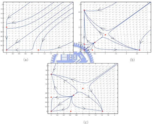
0 0.5 1 1.5 2 2.5 3 0 0.5 1 1.5 2 2.5 3 0 0.2 0.4 0.6 0.8 1 1.2 1.4 1.6 1.8 2 0 0.2 0.4 0.6 0.8 1 1.2 1.4 1.6 1.8 2 0 0.2 0.4 0.6 0.8 1 1.2 1.4 1.6 1.8 2 0 0.2 0.4 0.6 0.8 1 1.2 1.4 1.6 1.8 2 )d* )c* )b*

Figure 3: In figure (a), (0, 0) is stable equilibrium and (1, 0), (0, 1) are saddle points. (b) is for ˙xi(t) system, it has seven equilibria: three stable equilibria

are (0, 0), (2.168, 0), (0, 2.168), and four unstable equilibria are (1, 1), (0.5, 0.5), (0.382, 0), (0, 0.382). (c) is for ˙yi(t) system, ut has seven equilibria: three stable

equilibria are (0, 0), (1.618, 0), (0, 1.618), and four unstable equilibria are (1, 1), (0.707, 0.707), (0.618, 0), (0, 0.618) (in example 2.3).

In this section, for c = 0, there exists a stable equilibrium with all switches on, whose components are identically σ/(1 + n). For c = 1 and σ > 1, the manifold of equilibria (2.3) is stable and the origin is an unstable equilibrium.

Let c > 1.

(i) If (σ/c)c_{((c − 1)/k)}c−1 _{≥ 1, then there exist equilibria with k switches on with}

identical components, and (n − k) off (zero), for 1 ≤ k ≤ n. In addition, the equilibrium with one switch-on (k = 1), and n − 1 off (zero) exists if σ ≥ 2. (ii) The equilibrium with one switch-on of value a and (n − 1) off (zero) is stable,

if a > (c/σ)c−11 , and unstable if a < (c/σ)c−11 .

(iii) The above equilibria with k switch-on for 1 < k ≤ n are unstable.

Finally, the model is a gradient system, we also justify that for c ≥ 1/2, every solution of systems (2.1) tends to an equilibrium as time tends to infinity. .

3

Model with mutual inhibition, autocatalysis, and

leak

In this section, we add leak α > 0 to the equations (2.1), i.e., ˙ xi = −xi+ σx c i 1 +Pn_j=1xc j + α, 1 ≤ i ≤ n. (3.1)

If one component of the equilibrium is zero, then it contradicts the assumption α > 0. Thus, (0, 0, · · · , 0), (a, 0, 0, · · · , 0), (a, a, · · · , a, 0, 0, · · · , 0) can not satisfy the above equations. We have the origin, one switch on and (n − 1) off, k switches on with identical components (k > 1) and (n − k) off (zero) are not equilibria.

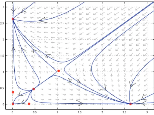
By the numerical illustrations, we guess that if the leak is small, then it does not have a major effect on the systems, except when the cooperativity is close to 1. To give an instance: when n = 2, c = 2, σ = 3, α = 0.01, i.e., the system is

( ˙ x1 = −x1+ 3x 2 1 1+x2 1+x22 + 0.01 ˙ x2 = −x2+ 3x 2 2 1+x2 1+x22 + 0.01 ,

then there exist seven equilibria (0,2.631), (2.631,0), (0.010,0.010), (0,0.368), (0.368,0), (0.471,0.471), (1.029,1.029). The first three are stable; the last four are unstable. The dynamical behavior in figure 4 is similar to (b) in figure 3.

0 0.5 1 1.5 2 2.5 3 0 0.5 1 1.5 2 2.5 3 x

Figure 4: If the leak is small, it does not have a major effect on the system. In addition, it has seven equilibria.

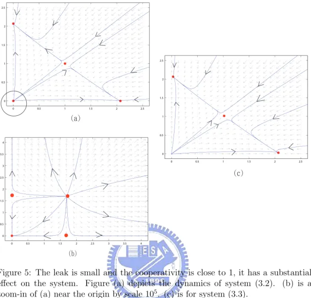
Moreover, we compare the system ( ˙ x1 = −x1+ 3x 1.1 1 1+x1.1 1 +x1.12 ˙ x2 = −x2+ 3x 1.1 2 1+x1.1 1 +x1.12 (3.2) with ₍ ˙ x1 = −x1+ 3x 1.1 1 1+x1.1 1 +x1.12 + 0.01 ˙ x2 = −x2+ 3x 1.1 2 1+x1.1 1 +x1.12 + 0.01 . (3.3)

In system (3.2), it has seven equilibria: (0,0), (0,2.070) and (2.070,0) are stable; (1,1), (0.00002,0.00002), (0,0.00002) and (0.00002,0) are unstable. In system (3.3), it has three equilibria: (0,2.085) and (2.085,0) are stable; (1.016,1.016) is unstable. The numbers of equilibria is clearly different. Thus, when the leak is small and the cooperativity is close to 1, it has a substantial effect on the systems (see figure 5).

Next, we consider three cases for c, i.e. c = 0, c = 1, and c > 1. If c = 0, then (3.1) becomes

˙

xi = −xi+

σ

1 + n+ α, 1 ≤ i ≤ n.

Proposition 3.1 : For c = 0, there exists a stable equilibrium with all switches on, whose components are identically α + σ/(1 + n).

Proof: Consider the existence of the equilibrium with all switches on, whose com-ponents are identical. Then (α + σ/(1 + n), α + σ/(1 + n), · · · , α + σ/(1 + n)) ∈ Rn

0 0.5 1 1.5 2 2.5 0 0.5 1 1.5 2 2.5 0 0.5 1 1.5 2 2.5 3 3.5 4 0 0.5 1 1.5 2 2.5 3 3.5 4 *W` b)g* 0 0.5 1 1.5 2 2.5 0 0.5 1 1.5 2 2.5 )d* )c* )b*

Figure 5: The leak is small and the cooperativity is close to 1, it has a substantial effect on the system. Figure (a) depicts the dynamics of system (3.2). (b) is a zoom-in of (a) near the origin by scale 105_{. (c) is for system (3.3).}

constant, it does not affect the linearization at the equilibrium. The result is similar to proposition 2.1. Hence, the equilibrium is stable. The assertion follows.

Next, consider c = 1, then (3.1) become dxi

dt = −xi+

σxi

1 +Pn_j=1xj

+ α, 1 ≤ i ≤ n.

Proposition 3.2 : For c = 1, there exists a stable equilibrium with all switches on, whose components are identically [−1 + nα + σ +p(1 − nα − σ)2_{+ 4nα]/2n.}

Proof: A steady state solution of the form (a, a, · · · , a) satisfies

−a + σa

1 + na + α = 0 or na

2_{+ (1 − nα − σ)a − α = 0,}

and the solution of above equation is [−1 + nα + σ +p(1 − nα − σ)2_{+ 4nα]/2n.}

Since α is constant, it does not affect the linearization at the equilibrium. From (2.2), the linearation at (a, a, · · · , a) is

      

−1 + σ(1+(n−1)a)_(1+na)2 _(1+na)−σa2 · · · _(1+na)−σa 2

−σa (1+na)2 −1 + σ(1+(n−1)a) (1+na)2 ... ... ... · · · . .. −σa (1+na)2 −σa

(1+na)2 · · · _(1+na)−σa 2 −1 +

σ(1+(n−1)a) (1+na)2        .

The eigenvalues for this matrix are

λ1 = −1 + σ(1 + (n − 1)a) (1 + na)2 + σa (1 + na)2, λ2 = −1 + σ(1 + (n − 1)a) (1 + na)2 − (n − 1)σa (1 + na)2. Note that

λ1 < 0 ⇔ σ(1 + na) < (1 + na)2 ⇔ σ < 1 + na. (3.4)

From the steady state equation, then 1 + na = σa/(a − α). With it to substitute for the inequality (3.4). We have σ < 1 + na = σa/(a − α), i.e., σα > 0. Hence, for c = 1, in any condition (since σ > 0 and α > 0), then (a, a, · · · , a) is stable. Thus, the assertion follows.

Example 3.1 : In proposition 3.2, if n = 2, σ = 2, and α = 1, i.e., the system is ½

˙

x1 = −x1+ _1+x2x_1+x1 ₂ + 1

˙

x2 = −x2+ _1+x2x_1+x2 ₂ + 1 ,

then (1.781,1.781) is a stable equilibrium since σα = 2 > 0 (see figure 6).

We consider c > 1 in the following discussions . There exist two kinds of stable equilibria. In proposition 3.3, we discuss the equilibrium with all switches on, whose components are identically less than cα/(c − 1). The other one is that the components consists of two different values. In proposition 3.4, we restrict to the

0 0.5 1 1.5 2 2.5 3 0 0.5 1 1.5 2 2.5 3

Figure 6: (1.781,1.781) is a stable equilibrium (in example 3.1).

case with dimension n = 2, 3; in proposition 3.5, we consider the case for dimension n ≥ 4.

The result of proposition 3.3 is sketched in [4]. We recast it with more details. Proposition 3.3 : For c > 1, there exist stable equilibrium with all switches on, whose components are identically a with a < cα/(c − 1).

Proof: A steady state solution of the form (a, a, · · · , a) satisfies −a + σa

c

1 + nac + α = 0

or nac+1_{− (σ + nα)a}c_{+ a = α. Set h(ζ) = nζ}c+1_{− (σ + nα)ζ}c_{+ ζ. We compute that}

h0_{(ζ) = n(c + 1)ζ}c_{− c(σ + nα)ζ}c−1_{+ 1}

h00_{(ζ) = nc(c + 1)ζ}c−1_{− c(σ + nα)(c − 1)ζ}c−2_.

Therefore, ζ = (σ + nα)(c − 1)/n(c + 1) is the reflection point. And h(ζ) → ∞ as ζ → ∞, and h(ζ) passes point (0, 0), We have the curve of the function h(ζ) is down in the left side of the reflective point and is upper in the other. Further, there is intersection of h(ζ) and horizontal line α. Thus, it there is one solution.

Next, consider the local stability of (a, a, · · · , a). Since α is constant, it does not affect the linearization at the equilibrium. From (2.7), we have the greatest eigenvalue is −1 + σcac−1_{/(1 + na}c_{). And with the above steady state equation, then}

1 + nac_{= σa}c_{/(a − α). If the greatest eigenvalue is negative, then σca}c−1 _{< 1 + na}c_.

We substitute 1 + nac _{for σa}c_{/(a − α) in the above inequality. Thus, (a, a, · · · , a) is}

We consider n = 2 and there exists an equilibrium (a, b) where a > b. Then (a, b) satisfies

½

ac+1_{− (α + σ)a}c_{+ (1 + b}c_{)a − α(1 + b}c_{) = 0}

bc+1_{− (α + σ)b}c_{+ (1 + a}c_{)b − α(1 + a}c_{) = 0} ,

and n = 3 and there exists equilibrium (a, a, b) where a > b. Then (a, a, b) satisfies ½

2ac+1_{− (2α + σ)a}c_{+ (1 + b}c_{)a − α(1 + b}c_{) = 0}

bc+1_{− (α + σ)b}c_{+ (1 + 2a}c_{)b − α(1 + 2a}c_{) = 0} ,

Proposition 3.4 : Let c > 1.

(i) If n = 2 and the equilibrium (a, b) exists. Then it is stable if σ2_c2_a2c−1_b2c−1 _<

(−(1 + ac_{+ b}c₎2_{+ σc(1 + b}c_)ac−1_{)(−(1 + a}c_{+ b}c₎2_{+ σc(1 + a}c_)bc−1_{), with one}

switch-on with value a, and one off with value b.

(ii) If n = 3, σcac−1 _{< 1 + 2a}c_{+ b}c _{and the equilibrium (a, a, b) exists. Then it is}

stable if 2σ2_c2_a2c−1_b2c−1 _{< (−(1 + 2a}c_{+ b}c₎2 _{+ σc(1 + 2a}c_)bc−1_{)(−(1 + 2a}c₊

bc₎2_{+ σc(1 + b}c_)ac−1_{), with two switches-on with value a identically, and one}

off with value b. In addition, if a change for b, then we have the condition of the stability for the equilibrium with one switch-on with value a, and two off with value b identically.

Proof: We analysis the stability for these equilibria. (i) From (2.2), the linearization at (a, b) is

à −1 + σc(1+pb_(1+ac_+bc)acc−1₎2 −σca c_bc−1 (1+ac_+bc₎2 −σcac−1_bc (1+ac_+bc₎2 −1 + σc(1+kac_)bc−1 (1+ac_+bc₎2 ! let = µ d u v m ¶ .

We have two eigenvalues are [d+m+p(d − m)2_{+ 4uv]/2 and [d+m−}p_{(d − m)}2_{+ 4uv]/2.}

If the larger is negative, i.e.,

σ2c2a2c−1b2c−1< (−(1 + ac+ bc)2+ σc(1 + bc)ac−1)(−(1 + ac+ bc)2+ σc(1 + ac)bc−1), then all eigenvalues are negative, i.e., (a, b) and (b, a) are stable.

(ii) From (2.2), the linearization at (a, a, b) is 

  

−1 + σc(1+a_(1+2ac+bc_+bc)ac₎c−12 −σca 2c−1 (1+2ac_+bc₎2 −σca c_bc−1 (1+2ac_+bc₎2 −σca2c−1 (1+2ac_+bc₎2 −1 + σc(1+ac_+bc_)ac−1 (1+2ac_+bc₎2 −σca c_bc−1 (1+2ac_+bc₎2 −σcbc_ac−1 (1+2ac_+bc₎2 −σcb c_ac−1 (1+2ac_+bc₎2 −1 + σc(1+2ac_)bc−1 (1+2ac_+bc₎2    let=   d r u_{r d u} v v m   .

We have three eigenvalues are d − r, [d + r + m +p(d + r − m)2_{+ 8uv]/2 and}

[d + r + m −p(d + r − m)2_{+ 8uv]/2. If d − r < 0 and 2uv < m(d + r), i.e.,}

σcac−1 _{< 1 + 2a}c_{+ b}c _and

2σ2_c2_a2c−1_b2c−1 _{< (−(1+2a}c_+bc₎2_+σc(1+2ac_)bc−1_)(−(1+2ac_+bc₎2_+σc(1+bc_)ac−1_),

then all eigenvalues are negative. Thus, (a, a, b), (a, b, a) and (b, a, a) are stable. In addition, if a change for b, then we have the condition of the stability for the equi-librium with one switch-on with value a, and two off with value b identically. Thus, the assertion follows.

Let p = n − k. The steady state solution of the form (a, a, · · · , a, b, b, · · · , b) with k0_{s a and p}0_{s b satisfies}

½

kac+1_{− (αk + σ)a}c_{+ (1 + pb}c_{)a − α(1 + pb}c_{) = 0}

pbc+1_{− (αp + σ)b}c_{+ (1 + ka}c_{)b − α(1 + ka}c_{) = 0} ,

We assume such equilibrium exist.

The following characteristic polynomial has been mentioned in [4] without computing eigenvalues for system (3.5). We provide linear stability analysis for these equilibrium in the following proposition 3.5.

Proposition 3.5 :For c > 1, n ≥ 4, k > 1, and the equilibrium (a, a, · · · , a, b, b, · · · , b) with k0_{s a and p}0_{s b exists. Then it is stable if σca}c−1_{< 1 + ka}c_{+ (n − k)b}c _{with k}

switches-on with value a identically, and (n − k) off with value b identically.

Proof: From(2.2), the linearization at (a, a, · · · , a, b, b, · · · , b) is                d r · · · r u · · · · u r d ... ... ... ... ... ... ... ··· ... r ... ... ... ... r · · · r d u · · · · u v · · · v m s · · · s ... ... ... ... s m ... ... ... ... ... ... ... ··· ... s v · · · v s · · · s m                (3.5)

where d = −1 + σc(1 + (k − 1)ac+ pbc)ac−1 (1 + kac_{+ pb}c₎2 , m = −1 + σc(1 + kac+ (p − 1)bc)bc−1 (1 + kac_{+ pb}c₎2 , r = −σca 2c−1 (1 + kac_{+ pb}c₎2, s = −σcb 2c−1 (1 + kac_{+ pb}c₎2, u = −σca c_bc−1 (1 + kac_{+ pb}c₎2, v = −σca c−1_bc (1 + kac_{+ pb}c₎2.

We do row operations and column operations.                d r · · · r u 0 · · · 0 r d ... ... ... ... ... ... ... ··· ... r ... ... ... ... r · · · r d u 0 · · · 0 v · · · v m s − m · · · s − m ... ... ... ... s m − s 0 ... ... ... ... ... . .. v · · · v s 0 m − s                →                d − r 0 r − d 0 0 · · · 0 . .. ... ... ... ... ... 0 d − r r − d 0 ... ... ... r · · · r d u 0 · · · 0 v · · · · · · v m s − m · · · s − m ... ... ... ... s m − s 0 ... ... ... ... ... . .. v · · · · · · v s 0 m − s                →

              d − r 0 r − d 0 0 · · · 0 . .. ... ... ... ... ... 0 d − r r − d 0 ... ... ... r · · · r d u 0 · · · 0 pv · · · · · · pv m + (p − 1)s 0 · · · 0 v · · · · · · v s m − s 0 ... ... ... ... ... . .. v · · · · · · v s 0 m − s               →               d − r 0 0 0 0 · · · 0 . .. ... ... ... ... ... 0 d − r 0 0 ... ... ... r · · · r d + (k − 1)r u 0 · · · 0 pv · · · pv kpv m + (p − 1)s 0 · · · 0 v · · · v kv s m − s 0 ... ... ... ... ... . .. v · · · v kv s 0 m − s               .

The characteristic polynomial of the matrix is

(m − s − x)p−1_{(d − r − x)}k−1_{((d + (k − 1)r − x)(m + (p − 1)s − x) − kpuv) =}

(m − s − x)p−1_{(d − r − x)}k−1_(x2_{− (d + m + (k − 1)r + (p − 1)s)x + dm + (p − 1)sd +}

(k − 1)mr + (k − 1)(p − 1)rs − kpuv). We have two eigenvalues are

d − r = −1 + σca

c−1

1 + kac_{+ pb}c,

m − s = −1 + σcbc−1 1 + kac_{+ pb}c.

If the larger is negative, then σcac−1 _{< 1 + ka}c_{+ pb}c_{. The others satisfy}

λ1+ λ2 = d + m + (k − 1)r + (p − 1)s

= (d − r) + (m − s) + kr + ps < 0, and

λ1λ2 = (p − 1)sd + (k − 1)mr + (k − 1)(p − 1)rs + dm − kpuv

= ps(d − r) + kr(m − s) + (s − m)(r − d) > 0.

So, if σcac−1 _{< 1 + ka}c_{+ pb}c_{, then all eigenvalues are negative, i.e., the equilibrium}

In proposition 3.6, the main result is proposed from [4], but we recast it with more details.

Proposition 3.6. ([4]) : For c ≥ 1/2, every solution of systems (2.1) tends to an equilibrium as time tends to infinity.

Proof: Let yi =√xi. Then ˙yi = ˙xi/2yi, i.e.,

˙yi = −xi+ σx c i 1+Pnj=1xcj + α 2yi = −y 2 i + σy2c i 1+Pnj=1yj2c + α 2yi = 1 2(−yi+ σy2c−1 i 1 +Pn_j=1y2c j + α yi ) = −∂V ∂yi , where V (yi) = 1 4 n X j=1 y2 j − σ 4clog(1 + n X j=1 y2c j ) − 1 2log( n Y j=1 yα j).

Thus ˙yi = ˙xi/2yi is a gradient system. Moreover

−yi+ σy2c−1_i 1 +Pn_j=1y2c j + α yi = 0 ⇔ −xi+ σxc i 1 +Pn_j=1xc j + α = 0.

By the Lasalle’s invariant principle [1], thus, every solution of the system converges to one of the equilibria as time tends to infinity. The assertion follows.

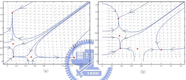
Example 3.2 : In proposition 3.3 and 3.4, if n = 2, c = 2, σ = 2 and α = 0.1, i.e., the system is ₍ ˙ x1 = −x1+ 2x 2 1 1+x2 1+x22 + 0.1 ˙ x2 = −x2+ 2x 2 2 1+x2 1+x22 + 0.1 . (3.6)

First, consider (a, a) is an equilibrium, we have

−a + 2a

2

1 + 2a2 + 0.1 = 0,

or 20a3 _{− 22a}2 _{+ 10a − 1 = 0, it only exists a real root. Thus, (0.135, 0.135) is a}

stable equilibrium since a = 0.135 < 0.2 = cα/(c − 1). Next, consider (a, b), and (b, a) are equilibria, we have

( −a + 2a2 1+a2_+b2 + 0.1 = 0 −b + 2b2 1+a2_+b2 + 0.1 = 0 .

By calculating, we have 100b4_−22b3_+121b2_{−20b+2 = 0, the solutions only have two}

real roots. Thus, there exist four equilibria: (0.107, 1.458), (1.458, 0.107), (0.122, 0.557), and (0.557, 0.122). The first two are stable and the last two are unstable since they satisfy the condition in proposition 3.4.

If consider yi =

√

xi, then the above system become

( ˙ y1 = 1₂(−y1+ 2y 3 1 1+y4 1+y24 + 0.1 y1) ˙ y2 = 1₂(−y2+ 3y 3 2 1+y4 1+y24 + 0.1 y2) . (3.7)

We see that the two systems (3.6) and (3.7) have same dynamical behavior (see figure 7). 0 0.2 0.4 0.6 0.8 1 1.2 1.4 1.6 0 0.2 0.4 0.6 0.8 1 1.2 1.4 1.6 x 0 0.2 0.4 0.6 0.8 1 1.2 1.4 1.6 0 0.2 0.4 0.6 0.8 1 1.2 1.4 1.6 y )c* )b*

Figure 7: (a) is for ˙xi(t) system and (b) is for ˙yi(t). They have same dynamical

behavior.

In this section, for any c, the origin, one switch on and (n − 1) off, k switches on with identical components k > 1 and (n − k) off (zero) are not equilibria. The result is different to section 2. For c = 0, there exists a stable equilibrium with all switches on, whose components are identically α + σ/(1 + n).

For c = 1, there exists a stable equilibrium with all switches on, whose com-ponents are identically [−1 + nα + σ +p(1 − nα − σ)2_{+ 4nα]/2n.}

For c > 1, there exist stable equilibrium with all switches on, whose compo-nents are identically lower than cα/(c − 1). It is also different to proposition 2.3. Moreover,

(i) If n = 2 and the equilibrium (a, b) exists. Then it is stable if σ2_c2_a2c−1_b2c−1 _<

(−(1 + ac_{+ b}c₎2_{+ σc(1 + b}c_)ac−1_{)(−(1 + a}c_{+ b}c₎2_{+ σc(1 + a}c_)bc−1_{), with one}

switch-on with value a, and one off with value b.

(ii) If n = 3, σcac−1 _{< 1 + 2a}c_{+ b}c _{and the equilibrium (a, a, b) exists. Then it is}

stable if 2σ2_c2_a2c−1_b2c−1 _{< (−(1 + 2a}c_{+ b}c₎2 _{+ σc(1 + 2a}c_)bc−1_{)(−(1 + 2a}c₊

bc₎2_{+ σc(1 + b}c_)ac−1_{), with two switches-on with value a identically, and one}

off with value b. In addition, if a change for b, then we have the condition of the stability for the equilibrium with one switch-on with value a, and two off with value b identically.

Finally, the model is a gradient system, we also justify that the global conver-gence for the system.

4

A model for bHLH proteins

In this section, consider the bHLH proteins model

˙ xi = −xi+ σ( atxi 1+Pnj=1xj) c Kc+ (₁₊Patnxi j=1xj) c, 1 ≤ i ≤ n

where Kc = αact is binding constant and at is a total quantity of activator. Set

D = 1 +Pn_j=1xj, the above equations become

˙ xi = −xi+ σxc i αDc_{+ x}c i , 1 ≤ i ≤ n (4.1) where α = Kc ac t ∈ R

+ _{is a measure of the harshness of the competition between}

switches. In the following, consider two cases for c, i.e. c = 1 and c = 2. When c = 1, then (4.1) become ˙ xi = xi(−1 + σ α(1 +Pn_j=1xj) + xi ), 1 ≤ i ≤ n. (4.2)

Note that the Jacobian matrix of the vector field is J = [Jij] with

Ji,i = −1 + σα(1 +Pn_j6=ixj) (α(1 +Pn_j=1xj) + xi)2 , (4.3) Ji,j = −σαxi (α(1 +Pn_j=1xj) + xi)2 for j 6= i.

In proposition 4.1, the result of (i) is new. In addition, the results of (ii) and (iii) are stated in [4], but we recast them with more details.

Proposition 4.1 : Let c = 1.

(i) If σ < α, then the origin is stable.

(ii) If σ > α and 1 ≤ k < n, then there exist unstable equilibria with k switches on, whose components are identically (σ − α)/(αk + 1), and (n − k) off (zero). (iii) There exists a stable equilibrium with all switches on, whose components are

identically (σ − α)/(αn + 1).

Proof: (i) The linearizaation at the origin is      −1 + σ α 0 · · · 0 0 −1 + σ α ... ... ... · · · . .. 0 0 · · · 0 −1 + σ α     . If −1 + σ

α < 0 or σ < α, then the origin is stable. The result follows.

(ii) The steady state equation for the (a, a, · · · , a, 0, 0, · · · , 0), a 6= 0 is an equilibrium if and only if

−a + σa

α(1 + ka) + a = 0,

i.e. a = (σ − α)/(αk + 1) > 0. Thus, σ > α is the condition of existence. From (4.3), the linearization at (a, a, · · · , a, 0, 0, · · · , 0) is

          

−1 + σα(1+(k−1)a)_(α(1+ka)+a)2 _(α(1+ka)+a)−σαa 2

. .. −σαa (α(1+ka)+a)2 −1 + σα(1+(k−1)a) (α(1+ka)+a)2 −σαa (α(1+ka)+a)2 0 −1 + σ α(1+ka) 0 . .. 0 −1 + σ α(1+ka)            .

So, −1 + σ/α(1 + ka) is a eigenvalue. To substitute a for (σ − α)/(αk + 1). Thus, the above eigenvalue becomes −1 + (σαk + σ)/(σαk + α). It always posi-tive. Moreover, when k = 1, the above result also holds. Thus, (a, 0, 0, · · · , 0) and (a, a, · · · , a, 0, 0, · · · , 0) are unstable equilibria. The result follows.

(iii) The steady state equation for the (a, a, · · · , a), a 6= 0 is an equilibrium if and only if

−a + σa

α(1 + na) + a = 0,

i.e., a = (σ − α)/(αn + 1) > 0. Thus, σ > α is the condition of existence. From (4.3), the linearization at (a, a, · · · , a) is

      

−1 + σα(1+(n−1)a)_(α(1+na)+a)2 _(α(1+na)+a)−σαa 2 · · · _(α(1+na)+a)−σαa 2

−σαa (α(1+na)+a)2 −1 + σα(1+(n−1)a) (α(1+na)+a)2 ... ... ... · · · . .. −σαa (α(1+na)+a)2 −σαa

(α(1+na)+a)2 · · · _(α(1+na)+a)−σαa 2 −1 +

σα(1+(n−1)a) (α(1+na)+a)2        .

By Lemma 2.1, the eigenvalues are

λ1 = −1 + σα(1 + na) (α(1 + na) + a)2, and λ2 = −1 + σα (α(1 + na) + a)2 < λ1. If λ1 is negative, then σα(1 + na) < (α(1 + na) + a)2.

To substitute a(αn + 1) for (σ − α), the above inequality becomes σα(1 + na) < σ2_.

i.e., a < (σ − α)/αn. It always holds since a = (σ − α)/(αn + 1). Hence, we have (a, a, · · · , a) is stable. The assertion follows.

Example 4.1 : In proposition 4.1, if n = 2, σ = 2 and α = 3, i.e., the system is (

˙

x1 = −x1+ _3(1+x12x_+x1_2)+x1

˙

x2 = −x2+ _3(1+x12x_+x2_2)+x2 ,

then (0, 0) is stable equilibrium, since it satisfies σ < α. Next, if n = 2, σ = 3 and α = 2, i.e., the system is

( ˙

x1 = −x1+ _2(1+x13x_+x1_2)+x1

˙

x2 = −x2+ _2(1+x13x_+x2_2)+x2 ,

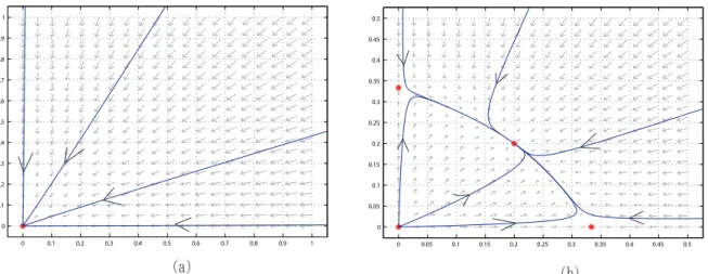
then there exist four equilibria: (0.2, 0.2) is stable; moreover, (0, 0), (1/3, 0), (0, 1/3) are unstable (see figure 8).

0 0.1 0.2 0.3 0.4 0.5 0.6 0.7 0.8 0.9 1 0 0.1 0.2 0.3 0.4 0.5 0.6 0.7 0.8 0.9 1 0 0.05 0.1 0.15 0.2 0.25 0.3 0.35 0.4 0.45 0.5 0 0.05 0.1 0.15 0.2 0.25 0.3 0.35 0.4 0.45 0.5 y )b* _)c*

Figure 8: In figure (a), (0, 0) is stable. In (b), (0.2, 0.2) is stable; moreover, (0, 0), (1/3, 0), (0, 1/3) are unstable (Example 4.1).

In the following, it is assumed that transcriptional activation occurs with co-operativity c = 2. The systems (4.1) become

˙ xi = −xi+ σx2 i αD2_{+ x}2 i (4.4) where D = 1 +Pn_j=1xj, and α = K_a22

t . The steady state equation is

xi = σx2 i αD2_{+ x}2 i or αD2_{+ x}2 i = σxi if xi 6= 0. Note that Ji,i = −1 + 2σαxi D(D − xi) (αD2_{+ x}2 i)2 = 1 − 2 σ(xi+ αD) if xi 6= 0, (4.5) Ji,j = −2αDσx2 i (αD2_{+ x}2 i)2 = −2αD σ if xi 6= 0 for all j 6= i.

Clearly, the origin is a stable equilibrium, since the linearization at the origin is      −1 0 · · · 0 0 −1 ... ... ... ··· ... 0 0 · · · 0 −1     .

In proposition 4.2, the results are stated in [4]. We provide detailed proof herein.

Proposition 4.2. ([4]) Let c = 2, and 1 ≤ k ≤ n.

(i) If 4α(kσ + 1)/σ2 _{≤ 1, then there exist equilibria with k switches on, whose}

components are identically [σ − 2αk +pσ2_{− 4α(kσ + 1)]/2(1 + αk}2_{) or [σ −}

2αk −pσ2_{− 4α(kσ + 1)]/2(1 + αk}2_{), and (n − k) off (zero). In short, the}

condition of existence is α < 1/k2_.

(ii) When k = 1, if the non-zero components are larger than (σ − 2α)/2(1 + α), then the above equilibria are stable.

(iii) When 1 < k ≤ n, if the non-zero components are larger than α/2, then the above equilibria are stable. In short, the condition of stability is σ > 2√α/(1 − k√α).

Proof: (i) The steady state equation for (a, a, · · · , a, 0, 0, · · · , 0), a 6= 0 is an equi-librium if and only if

−a + σa2

α(1 + ka)2_{+ a}2 = 0

i.e.,

a2_{(1 + αk}2_{) + a(2αk − σ) + α = 0 if a 6= 0.}

The solutions are

a = σ − 2αk ± p

σ2_{− 4α(kσ + 1)}

2(1 + αk2₎ .

A sufficient and necessary condition for the existence is 4α(kσ+1)/σ2 _{≤ 1. However,}

from (4.4), we have

a2_{− σa + αD}2 _{= 0.}

The only solution is a = (σ +√σ2_{− 4αD}2_{)/2, where D ≤ σ/2}√_{α. Note that}

D − 1 = n(σ + √ σ2 _{− 4αD}2 2 ), it can rearranged to 2 + nσ + n√σ2_{− 4αD}2 _{≤ √}σ α.

It follows that nσ < σ/√α, or α < 1/n2_{. Since α < 1/n}2 _{< 1/k}2_{. In short, the}

condition of existence is α < 1/k2_.

(ii) From (4.5), the linearization at (a, 0, 0, · · · , 0) is      1 − 2 σ(a + α(1 + a)) − 2α(1+a) σ 0 −1 0 . .. 0 −1     .

If 1 − 2(a + α(1 + a))/σ is negative, then all eigenvalues are negative. Thus, if a > (σ − 2α)/2(1 + α), then this equilibrium is stable.

(iii) First, consider k = n, from (4.5), the linearization at (a, a, · · · , a) is       1 − 2 σ(a + α(1 + na)) −2α(1+na) σ · · · −2α(1+na) σ −2α(1+na) σ 1 − 2 σ(a + α(1 + na)) ... ... ... · · · . .. −2α(1+na)_σ −2α(1+na) σ · · · −2α(1+na) σ σ2(a + α(1 + na))      .

By Lemma 2.1, the eigenvalues are

λ1 = 1 − 2a σ , and λ2 = 1 − 2a + 2αn(1 + na) σ < λ1.

If λ1 < 0, i.e., a > σ/2, then (a, a, · · · , a) is stable. To replace with the solution, we

have

σ − 2αn +pσ2_{− 4α(nσ + 1) > σ + n}2_ασ.

The solution of the equation

(1 − n4_α2_)σ2_{− (4αn + 4n}3_α2_{)σ − 4α − 4n}2_α2 _{> 0}

are σ > 2√α/(1 − n√α).

Next, consider 1 < k < n, the linearization at (a, a, · · · , a, 0, 0, · · · 0) is           1 − 2(a+α(1+ka))_σ −2α(1+ka)_σ . .. −2α(1+ka) σ 1 − 2(a+α(1+ka)) σ −2α(1+ka) σ 0 −1 0 . .. 0 −1          

Since σ > 2√α/(1 − n√α) > 2√α/(1 − k√α), then (a, a, · · · , a, 0, 0, · · · 0) is also stable. The assertion follows.

In proposition 4.3, the results are stated in [4]. We provide detailed proof herein.

Proposition 4.3. ([4]) For c = 2, n ≥ 4, and k > 1, there exist unstable equilibria with k switches on with value a identically, and (n − k) off with value b identically.

Proof: Without loss of generality, assume a > b. By the steady state equation, a2_{− σa = b}2_{− σb}

or (a − b)(a + b − σ) = 0, we have a + b = σ. Let p = n − k, from (4.5), the linearization at (a, a, · · · , a, b, b, · · · , b) is           σ−2(a+α(1+ka+pb)) σ −2α(1+ka+pb) σ . .. −2α(1+ka+pb) σ σ−2(a+α(1+ka+pb)) σ −2α(1+ka+pb) σ −2α(1+ka+pb) σ σ−2(b+α(1+ka+pb)) σ −2α(1+ka+pb) σ . .. −2α(1+ka+pb) σ σ−2(b+α(1+ka+pb)) σ          

By Lemma 2.1, we have 1 − 2b/σ is a eigenvalue. If it is negative, then b > σ/2 which contradicts the assumption. Thus, the assertion follows.

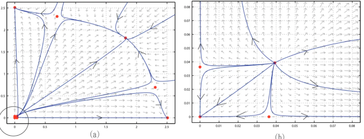
Example 4.2 : In proposition 4.2 and 4.3, if n = 2, σ = 3 and α = 0.1, i.e., the system is ₍ ˙ x1 = −x1+ 3x 2 1 0.1(1+x1+x2)2+x21 ˙ x2 = −x2+ 3x 2 2 0.1(1+x1+x2)2+x22 ,

then there exist nine equilibria: four equilibria are stable and five are unstable. We have (0, 0) is stable. (2.509, 0) and (0, 2.509) are stable since (14 +√185)/11 ≈ 2.509 > (σ − 2α)/2(1 + α) ≈ 1.727. (1.853, 1.853) is also stable since it satisfies σ = 3 > 2α/(1 − √α) ≈ 1.721. These equilibria (2.475, 0.525), (0.525, 2.475), (0.652, 0.652), (0.036, 0), (0, 0.036) are unstable (see figure 9).

0 0.5 1 1.5 2 2.5 0 0.5 1 1.5 2 2.5 0 0.01 0.02 0.03 0.04 0.05 0.06 0.07 0.08 0 0.01 0.02 0.03 0.04 0.05 0.06 0.07 0.08 )b* _)c*

Figure 9: Figure (b) is a zoom-in of (a) near the origin. There exist nine equi-libria: four equilibria are stable and five are unstable. We have (0, 0), (2.509, 0), (0, 2.509) and (1.853, 1.853) are stable. These equilibria (2.475, 0.525), (0.525, 2.475), (0.652, 0.652), (0.036, 0), (0, 0.036) are unstable.

(i) If σ < α, then the origin is stable.

(ii) If σ > α and 1 ≤ k < n, then there exist unstable equilibria with k switches on, whose components are identically (σ − α)/(αk + 1), and (n − k) off (zero). (iii) There exists a stable equilibrium with all switches on, whose components are

identically (σ − α)/(αn + 1). For c = 2, and 1 ≤ k ≤ n.

(i) If 4α(kσ + 1)/σ2 _{≤ 1, then there exist equilibria with k switches on, whose}

components are identically [σ − 2αk +pσ2_{− 4α(kσ + 1)]/2(1 + αk}2_{) or [σ −}

2αk −pσ2_{− 4α(kσ + 1)]/2(1 + αk}2_{), and (n − k) off (zero). In short, the}

condition of existence is α < 1/k2_.

(ii) When k = 1, if the non-zero components are larger than (σ − 2α)/2(1 + α), then the above equilibria are stable.

(iii) When 1 < k ≤ n, if the non-zero components are larger than α/2, then the above equilibria are stable. In short, the condition of stability is σ > 2√α/(1 − k√α).

In addition, when c = 2, n ≥ 4, and k > 1, there exist unstable equilibria with k switches on with value a identically, and (n − k) off with value b identically.

References

[1] Hale, Jack K., Ordinary Differential Equations. Malabar, Florida : Robert E. Krieger, 1980.

[2] Herbert Amann, Ordinary Differential Equations: An Introduction to Nonlinear Analysis. Walter de Gruyter and Co., Berlin·New York 1983.

[3] Cherry, J., Adler, F., 2000, How to make a biological switch, J. Theor. Biol. 203 (2), 117-133.

[4] Olivier Cinquin and Jacques Demongeot, High-dimensional switches and the modelling of cellular differentiation. Journal of Theoretical Biology 233(2005) 391-411.

[5] Olivier Cinquin and Karen M. Page, Generalized, Switch-Like Competitive Het-erodimerization Networks, Bulletin of Mathematical Biology (2007) 69: 483-494. [6] Stephen H. Friedberg, Arnold J, Insel, Lawrenle E. Spence, Linear Algebra.

Pearson Education. Inc 2003.

[7] Yates, A., Callard, R., and Stark, J., 2004, Combining cytokine signaling with T-bet and GATA-3 regulation in Th1 and Th2 differentiation: a model for cellular decision-making, J. Theor. Biol., 231, 181–196.