多電子系統於半導體量子點上之數值研究

國

立

交

通

大

學

應用數學系

博

士

論

文

多電子系統於半導體量子點上之數值研究

Numerical Studies of the Many-Electron System

in Semiconductor Quantum Dots

研 究 生：陳人豪

多電子系統於半導體量子點上之數值研究

Numerical Studies of the Many-Electron System

in Semiconductor Quantum Dots

研 究 生：陳人豪 Student：Jen-Hao Chen

指導教授：劉晉良 Advisor：Jinn-Liang Liu

國 立 交 通 大 學

應 用 數 學 系

博 士 論 文

Submitted to Department of Applied Mathematics College of Science

National Chiao Tung University in partial Fulfillment of the Requirements

for the Degree of Doctor of Philosophy

in

Applied Mathematics May 2007

Hsinchu, Taiwan, Republic of China

多電子系統於半導體量子點上之數值研究

學生：陳人豪 指導教授：劉晉良 教授

國立交通大學應用數學系博士班

摘 要

本論文分為兩部份，在第一個部分，我們利用電流自旋密度

泛函理論，對於三個垂直排列成一行的半導體量子點提出了

一個理論模型，並利用一些數值方法來探究。此量子點分子

模型是由三度空間中的硬牆侷限位能以及外部磁場所組成，

由於非拋物能帶有效質量的採用，多電子的 Hamiltonian 在

有限差分法下，會導出一個三次特徵值問題。而我們利用自

恰法來獲得在量子點分子中六個電子的 Kohn-Sham 軌域及

能量，其中薛丁格方程與卜易松方程分別由 Jacobi-Davidson

方法與 GMRES 所解出，從數值結果中，我們可以得知原本

在無磁場下，六個電子都位於中間的量子點，但在施加適當

之磁場後，每一個量子點都有兩個電子，Förster-Dexter 共振

能量轉換效應也許因此可由兩個量子點分子所形成，並提供

量子計算中費米量子位元一個新的設計概念。

在第二個部份，我們對半導體量子點中多電子的 Hamiltonian

之精確對角化提出了一個新的方法，由於我們的量子點模型

是由三度空間的硬牆侷限位能以及非拋物能帶有效質量所

組成，因此一些解析基底，例如拉格爾多項式，在此類模型

中是無法使用。在本方法中，我們利用單電子波函數所組成

的 Slater 行列式基底來建構多電子系統之波函數，其中單電

子 Hamiltonian 中使用了一個與能量及位置相關的有效質量，

並加入了適當的邊界條件，利用有限差分法，同樣也得到了

一個三次特徵值問題，並且亦透過 Jacobi-Davidson 方法來解

，而多電子 Hamiltonian 中的庫倫矩陣元素則是透過解卜易

松問題來獲得，我們的數值結果呈現只須少許的單電子基底

便可得到一個良好的收歛狀態。

Numerical Studies of the Many-Electron System

in Semiconductor Quantum Dots

Student：Jen-Hao Chen Advisor：Dr. Jinn-Liang Liu

Department of Applied Mathematics

National Chiao Tung University

ABSTRACT

This thesis consists of two parts. In the first part, based on the current

spin density functional theory, a theoretical model of three vertically

aligned semiconductor quantum dots is proposed and numerically studied.

This quantum dot molecule (QDM) model is treated with realistic

hard-wall confinement potential and external magnetic field in

three-dimensional setting. Using the effective-mass approximation with

band nonparabolicity, the many-body Hamiltonian results in a cubic

eigenvalue problem from a finite difference discretization. A

self-consistent algorithm for solving the Schrödinger-Poisson system by

using the Jacobi-Davidson method and GMRES is given to illustrate

the Kohn-Sham orbitals and energies of six electrons in the molecule

with some magnetic fields. It is shown that the six electrons residing

in the central dot at zero magnetic field can be changed to such that

each dot contains two electrons with some feasible magnetic field. The

Förster-Dexter resonant energy transfer may therefore be generated by

two individual QDMs. This may motivate a new paradigm of Fermionic

qubits for quantum computing in solid-state systems.

In the second part, we propose a new approach to the exact diagonal-

ization of many-electron Hamiltonian in semiconductor quantum dot (QD)

structures. The QD model is based on realistic 3D finite hard-wall

confinement potential and nonparabolic effective mass approximation

that render analytical basis functions such as Laguerre polynomials

inaccessible for the numerical treatment of this kind of models. In this

approach, the many-electron wave function is expanded in a basis of

Slater determinants constructed from numerical wave functions of the

single-electron Hamiltonian with the energy and position dependent

electron effective mass approximation and suitable boundary conditions

which result in a cubic eigenvalue problem from a finite difference

discretization. The nonlinear eigenvalue problem is also solved by using

the Jacobi-Davidson method. The Coulomb matrix elements in the

many-electron Hamiltonian are obtained by solving Poisson’s problems

via GMRES. Numerical results reveal that a good convergence can be

achieved by means of a few single-electron basis states.

致 謝

本論文得以完成，首先要感謝恩師 劉晉良教授多年來

的悉心指導與策勵支持，老師除了卓越的專業知識外，其嚴

謹的治學態度與追求新知的熱誠，更是學生在研究旅程上永

遠的標竿。師恩浩瀚，學生必永記於心。

論文口試期間，承蒙林文偉教授、賴明治教授、葉立明

教授、陳宜良教授、簡澄陞教授與呂宗澤教授等諸位審查委

員，對本論文提供許多寶貴的意見與指正，使論文更甄完善

，學生特此僅致誠摯的謝意。此外，亦感謝系上的老師、助

理、同學們曾經給予的協助與鼓勵。

感謝父親陳鴻基先生、母親黃淑英女士的養育之恩與用

心栽培，讓我能無後顧之憂的完成學業。要特別感謝是太太

孔驪，一路任勞任怨的付出與扶持，給予莫大的鼓勵讓我得

以倘佯在研究的旅程中。感謝妹妹幸宜與妹婿稟鎔的關心及

替遠在外地求學的我照顧父母。也要感謝岳父劉家霖先生與

岳母楊鳳霞女士願意將您的女兒嫁給尚未立業的我。最後，

僅以此論文獻給曾經幫助、關心過我的人，並再一次向恩師

劉晉良教授致上最深的謝意。

Contents

Abstract (in Chinese) ... i

Abstract (in English) ... iii

Acknowledgements (in Chinese) ... vi

Contents ... vii

List of Figures ... ix

I A Model for Semiconductor Quantum Dot Molecule Based on

the Current Spin Density Functional Theory

1 Introduction ... 1

2 The Current Spin Density Functional Theory for the Model System 5

3 Numerical Methods and Algorithms for the Model System .... 12

4 Numerical Results ... 22

5 Concluding Remarks ... 28

II A Numerical Method for Exact Diagonalization of Semicon-

ductor Quantum Dot Model

6 Introduction ... 31

7 Single-Electron Model ... 36

8 Numerical Methods for Single Electron Wave Functions ... 38

9 Many-Electron Model ... 41

... 43

10 Numerical Methods for Coulomb Matrix Elements ... 47

12 Concluding Remarks ... 57

13 Conclusions ... 58

Appendix ... 61

List of Figures

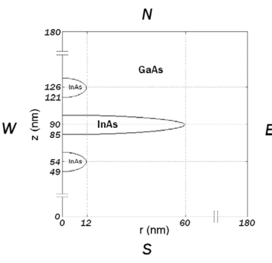
1.1 Three vertically aligned InAs/GaAs quantum dots with cylindri-cally symmetric domain in real space dimensions in nano meters that are used in numerical implementation. The domian in 2D set-ting is denoted by Ω with the boundary ∂Ω consisset-ting of the south (S), east (E), north (N), and west (W) sides. . . 4

4.1 The effect of the domain size on the first three energies at B = 0. 26 4.2 Contour of KS orbitals at B=0 (left panel) and B=15 (right panel). 27

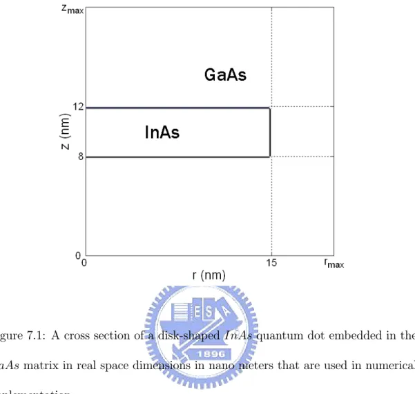
7.1 A cross section of a disk-shaped InAs quantum dot embedded in the GaAs matrix in real space dimensions in nano meters that are used in numerical implementation. . . 37

11.1 The effect of the domain size on the ground state energy of two-electron system with the basis size Ns = 8. . . 55 11.2 The ground state energies of two- and four-electron QDs as a

Part I

A Model for Semiconductor

Quantum Dot Molecule Based on

the Current Spin Density

Chapter 1

Introduction

There is significant interest in quantum information processing based on Fermi-onic qubits using semiconducting materials [1-10]. One of the proposals in this approach is to exploit electronic excitations of coupled quantum dots (QDs) that form an artificial molecule (QDM) [6] [7] [9] [10]. In particular, an energy selective scheme to manipulating excitonic states of QDM, together with control over the F¨orster-Dexter resonant energy transfer and biexciton binding energy, can be used to perform quantum computation and to produce controlled exciton quantum en-tanglement [7] [11]. The resonant F¨orster-Dexter energy transfer mechanism is also responsible for photosynthetic energy process in antenna complexes, biosys-tems that harvest sunlight [12]. It has been recently shown that two individual closely spaced fluorescent molecules undergo a strong coherent dipole-dipole cou-pling can produce entangled states [13]. We propose and numerically investigate here a theoretical model of three vertically aligned InAs/GaAs QDM whose di-mensions are commensurable with that of [9] in which a transmission electron micrograph of a QDM sample is illustrated.

above and beneath the central dot whose geometrical dimensions are shown in Fig. 1.1 where the radius, thickness, and separation of each dot are indicated by coordinates. It has been demonstrated in [11] [14] that there exists F¨orster energy transfer from smaller to larger dots via electrostatic coupling. Our goal for this model system is to investigate the detailed electronic properties of the QDM with N = 6 electrons under the effects of an external magnetic field by using the current spin density functional theory (CSDFT) [15] [16].

For the many-body Hamiltonian of our QDM model, we extend the models used in [17-19], which are based on parabolic one-band effective-mass envelope function approximation with either infinite or quadratic confinement potentials, to a more realistic finite confinement potential with band nonparabolicity that leads to an energy-dependent mass in the Hamiltonian for electrons. The non-parabolicity is derived from a projection from the eight-band Kane Hamiltonian into the 2_{× 2 conduction space and hence gives more accurate results as shown} in [20-23].

The CSDFT applied to the QDM system with three-dimensionality of the finite confinement and band nonparabolicity poses a very challenging task for the numerical implementation. The energy-dependent mass in the Hamiltonian results in a cubic eigenvalue problem from, e.g., a finite difference discretization. The Jacobi-Davidson (JD) method developed in [24] [25] is extended and incorporated into a self-consistent algorithm for solving the Schr¨odinger-Poisson system that

implements the CSDFT in real space. We also give a detailed description of the computational algorithm, the Poisson solver, and the approximation methods for the exchange-correlation (xc) energy.

Numerical results on the Kohn-Sham (KS) orbitals and energies of six elec-trons in the molecule with some magnetic fields are presented in detail. It is shown that the six electrons residing in the central dot at zero magnetic field can be changed to such that each dot contains two electrons with some feasible magnetic field. The F¨orster energy transfer may therefore be generated by two individual QDMs. This may motivate a new paradigm of Fermionic qubits for quantum computing in solid-state systems, which will be reported in a coming paper.

Figure 1.1: Three vertically aligned InAs/GaAs quantum dots with cylindrically symmetric domain in real space dimensions in nano meters that are used in nu-merical implementation. The domian in 2D setting is denoted by Ω with the boundary ∂Ω consisting of the south (S), east (E), north (N), and west (W) sides.

Chapter 2

The Current Spin Density

Functional Theory for the Model

System

The density functional theory (DFT) introduced in the two seminal papers [26] [27] is perhaps the most successful approach to compute the electronic structure of matter ranging from atoms, molecules, to solids. Vignale and Rasolt developed an extension of DFT that makes it possible to include gauge fields in the energy functional [15] [16] and has been widely used to describe the electronic structure of quantum dots in magnetic fields [17] [18] [19] [28].

In CSDFT, the ground state energy of an interacting system with electron number N and the total spin S in the local external potential Vext(r) is a functional of spin density nσ(r), with σ =_{↑, ↓ (or ±1) denoting spin-up and spin-down,} respectively,

E (n) = T (n) + n(r) Vext(r)+ 1

2VH(r) dr + EB(n) + Exc(n) , (2.1) where the total density n(r) =n↑_(r)+n↓_{(r) and the spin densities satisfy the} con-straint nσ(r)dr =Nσ with N↑ = (N + 2S) /2, and N↓ = (N _{− 2S) /2 [28].} As-suming that the ground state of the noninteracting reference system is nondegen-erate, the noninteracting kinetic energy is expressed as

T (n) = j,σ Ψjσ Π 1 2m(r,εjσ) Π Ψjσ , (2.2)

where Π = _{−ih∇ + eA(r) denotes the electron momentum operator, h is the} reduced Planck constant, e is the proton charge, A(r) = B₂ (_{−y, x, 0) is the} vec-tor potential induced by an external magnetic field B = curl A = Bz applied perpendicular to the xy plane, and Ψjσ and εjσ are Kohn-Sham (KS) orbitals and eigenvalues to be specified below. The effect of band nonparabolicity leads to the mass depending on both energy and position, which is defined by [20]

1 m(r,εjσ) = p 2 h2 2 εjσ+ Eg(r)−Vext(r) + 1 εjσ+ Eg(r)−Vext(r) + ∆(r) , (2.3)

where Eg(r) and ∆(r) are energy-band gap and spin-orbit splitting in the valence band, respectively, and p is the momentum matrix element. These parameters are material (position) dependent. We denote the spatial domain of the model, i.e., Fig. 1.1, as Ω = ΩInAs∪ ΩGaAs ⊂ R3, where the three InAs quantum dots are

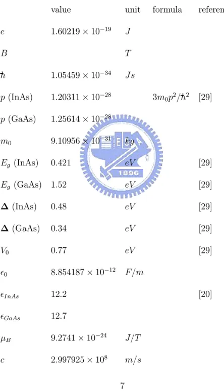
embedded in the GaAs matrix. All numerical values of the parameters used in this thesis are listed in Table 1, which also includes the corresponding units and cited references.

Table 1. Numerical values of all parameters used in this thesis. value unit formula reference e 1.60219_{× 10}−19 _J B T h 1.05459_{× 10}−34 _Js p (InAs) 1.20311_{× 10}−28 _3m 0p2/h2 [29] p (GaAs) 1.25614_{× 10}−28 m0 9.10956× 10−31 kg Eg (InAs) 0.421 eV [29] Eg (GaAs) 1.52 eV [29] ∆ (InAs) 0.48 eV [29] ∆ (GaAs) 0.34 eV [29] V0 0.77 eV [29] 0 8.854187× 10−12 F/m InAs 12.2 [20] GaAs 12.7 µB 9.2741× 10−24 J/T c 2.997925_{× 10}8 _m/s

The hard-wall confinement potential Vext is induced by a discontinuity of conduction-band edge of the system components and is given as

Vext(r) = ⎧ ⎪ ⎪ ⎪ ⎨ ⎪ ⎪ ⎪ ⎩ 0, in ΩInAs V0, in ΩGaAs. (2.4)

The Hartree potential is defined as

VH(r) = e2 4π 0 (r)

n(r )

|r − r |dr , (2.5) where 0 the permittivity of vacuum and (r) is the dielectric constant of the background material.

The vector field A(r) adds extra terms to the energy functional as follows

EB(n) = 1

2gµBB n

↑_(r)−n↓_{(r) dr+e j}

p(r)· A(r)dr, (2.6) where g is the Land´e factor, µB is the Bohr magneton, and

jp(r) =−ih 2m _j,σ Ψ

∗

jσ(r)∇Ψjσ(r)− Ψjσ(r)∇Ψ∗jσ(r) is the paramagnetic current density.

The xc energy Exc(n) is defined as

Exc(n) = Ex(n) + Ec(n) = n(r)εxc(n, γ) dr, (2.7)

where the xc energy per particle εxc depends on the field B. This is a conse-quence of the fact that the external field changes the internal structure of the wave function. It formally depends on the vorticity

γ(r) = _{∇ ×} jp(r)

n(r) _z. (2.8)

To minimize the total energy of the system, a functional derivative of E (n) is taken with respect to Ψ∗jσ under the constraint of the orbitals Ψjσ being normal-ized. The resulting KS equations are

Hσ_KSΨjσ = εjσΨjσ (2.9)

with the KS Hamiltonian HσKS defined as

Hσ_KS =_−Π 1 2m(r,εjσ) Π + Vext(r)+VB(r)+VH(r)+Vxcσ(r), (2.10) where VB(r) = σ 1 2g(r,εjσ)µBB, (2.11) g(r,εjσ) = 2 1− m0 m(r,εjσ) ∆(r) 3 (εjσ+ Eg(r)−Vext(r)) + 2∆(r) , (2.12)

and σ =_{±1 referring to the orientation of the electron spin along the z axis. The} xc potential

V_xcσ(r) = δ [n(r)εxc(n, γ)] δnσ −

e

njp· Axc, (2.13) where Axc is the xc vector potential defined by

eAxc= 1 n ∂ ∂y δ [n(r)εxc(n, γ)] δγ , − ∂ ∂x δ [n(r)εxc(n, γ)] δγ , 0 . (2.14) We use the LSDA for calculating the xc energy. In CSDFT, the LSDA has to be extended to include the orbital currents. Following Vignale and Rasolt [16], the xc vector potential is approximated as

e cAxc,σ ≈ −b nσ(r)∇ × ∇ × jpσ(r) nσ(r) , (2.15) where −b = mkF 48π2 χL χ0 L − 1 (2.16)

with kF being the Fermi momentum and χ_χL0

L the diamagnetic-susceptibility ratio.

The values of this ratio are tabulated in [30].

For the xc energy functional εxc in (2.13), we adopt the form developed by Perdew and Wang [31] as

εP Wxc (n, ζ) = εx(rs, ζ) + εc(rs, ζ) (2.17) where εx(rs, ζ) = − 3 4πrs 9π 4 1/3 _{(1 + ζ)}4/3_{+ (1− ζ)}4/3 2 , (2.18) εc(rs, ζ) = εc(rs, 0) + αc(rs) f (ζ) f (0) 1− ζ 4

+ [εc(rs, 1)− εc(rs, 0)] f (ζ)ζ4, (2.19)

ζ = n↑_(r)−n↓_{(r) /n(r) is the spin polarization, r}

s = _4πn3 1/3

is the Wigner-Seitz radius, and the functions εc(rs, 0), εc(rs, 1), and −αc(rs) are given in [31]. Note that the magnetic field dependence on the correlation energy, which might affect the total energies and spin configurations, is not taken into account in the present formula.

Chapter 3

Numerical Methods and

Algorithms for the Model System

Since the three QDs and the magnetic field are cylindrically symmetric, the wave function, the spin density, and the paramagnetic current density can be repre-sented as Ψq(r) = e−ilθφq(r, z) , q ≡ {nlσ} (3.1) nσ(r) = nσ(r, z) = Nσ q |φ q(r, z)|2, (3.2) jp(r) = − h m(r, z, εq) N q l_|φq(r, z)| 2 eθ, (3.3)

where n is the principal quantum number, l = 0,_{±1, ±2, · · ·, is the quantum} number of the projection of angular momentum onto the magnetic field axis, i.e., the z-axis and eθ is the azimuthal unit vector. The KS equations are then reduced to a 2D problem in the (r, z) coordinates as

where the KS Hamiltonian is now defined by Hlσ_KS = TS+ TB+ Vext+ VB+ VH+ Vxc (3.5) TS(r, z) = − h2 2m(r, z, εq) ∂2 ∂r2 + 1 r ∂ ∂r − l2 r2 + ∂2 ∂z2 (3.6) TB(r, z) = e2B2r2 8m(r, z, εq) + heBl 2m(r, z, εq) . (3.7)

In 2D setting, the solution domain for (3.4) is again expressed by the same notation as that of 3D, that is, Ω = ΩInAs ∩ ΩGaAs ⊂ R2. We choose the domain ΩGaAs sufficiently large so that the wave function is negligibly small at the boundary of ΩGaAs. By symmetry, the domain Ω can be reduced to Ω = _{{(r, z) : 0 ≤ r ≤ r}max,−zmax ≤ z ≤ zmax} for sufficiently large rmax > 0 and zmax > 0 as shown in Fig. 1.1.

The explicit formula for the potential Vxc(r) in (2.13) is extremely complex in 3D coordinates. Transforming it to the (r, z) space is prohibitively lengthy and impractical. We use all the original formulas (2.13)-(2.19) for calculating Vxc(r) in the 3D space and then obtain the potential in the (r, z) coordinates, i.e., Vxc(r, z) for (3.4).

Since we are dealing with the hard-wall confinement potential, the interface conditions of the wave function in (3.4) has to be specifically imposed, namely,

⎧ ⎪ ⎪ ⎪ ⎨ ⎪ ⎪ ⎪ ⎩ 1 2m(r,z,εq)Πφq(r, z)· n _Γ− = 1 2m(r,z,εq)Πφq(r, z)· n_Γ+, φq(r, z)|_Γ− = φq(r, z)|_Γ+, (3.8)

where Γ denotes the interface between two materials, i.e., Γ = ΩInAs∩ ΩGaAs, n is an outward normal unit vector on the boundary of ΩInAs, and Γ− and Γ+are the sets of limiting points to the curve Γ from the interior and the exterior of ΩInAs, respectively. The momentum operator Π is similarly defined for the 2D case. The boundary conditions for (3.4) are

⎧ ⎪ ⎪ ⎪ ⎨ ⎪ ⎪ ⎪ ⎩ ∂φq(r,z) ∂r _W = 0, φq(r, z) = 0, on S, E, N, (3.9)

where W , S, E, and N denotes the west, south, east, and north side boundaries of the domain Ω. Note that on the west side of the boundary the values of the wave function are taken to be the same for satisfying the continuity condition across W . In actual implementation this condition is replaced by taking the values of the two horizontal grid points adjacent to W as the same. Moreover, to avoid numerical over-flow due to the term 1/r in (3.6), we do not define unknowns at the grid points on W .

Note that the potential functions Vext(r) and VB(r) can be directly reduced to the (r, z) space since these functions are independent of the azimuthal coordinate. In real space approximation, the Hartree potential VH(r) is usually calculated by solving the Poisson equation [32]

∇ · (r)∇VH(r) =− e2 4π 0

n(r). (3.10)

∂2 ∂r2 + 1 r ∂ ∂r + 1 r2 ∂2 ∂θ2 + ∂2 ∂z2 VH(r, θ, z) = f (r, z), (3.11) f (r, z) = ₋ e 2 4π 0 i N q |φq(r, z)|2, for i = 1 or 2, (3.12)

where 1 = InAs if (r, z)∈ ΩInAs and 2 = GaAs if (r, z)∈ ΩGaAs. By using the method of separating variables and substituting a solution of the form

VH(r, θ, z) = VH(r, z) V (θ) (3.13) into (3.11), we have V (θ) ∂ 2 ∂r2 + 1 r ∂ ∂r + ∂2 ∂z2 VH(r, z) + VH(r, z) 1 r2 ∂2_{V (θ)} ∂θ2 = f (r, z) or V (θ)r2 VH(r, z) ∂2 ∂r2 + 1 r ∂ ∂r + ∂2 ∂z2 VH(r, z) + ∂2_{V (θ)} ∂θ2 = r2 VH(r, z) f (r, z). (3.14)

Obviously, by setting V (θ) = k where k is an arbitrary constant, a function VHp(r, z) = kVH(r, z) satisfying the 2D Poisson equation

∂2 ∂r2 + 1 r ∂ ∂r + ∂2 ∂z2 V p H(r, z) = f (r, z) (3.15) is a particular solution of (3.14) in view of a second order nonhomogeneous or-dinary differential equation with respect to θ. The corresponding homogeneous general solution is eikθ_Vh

∂2 ∂r2 + 1 r ∂ ∂r + ∂2 ∂z2 − k2 r2 V h H(r, z) = 0. (3.16) The general solution of the nonhomogeneous equation (3,14) is therefore of the form

k

eikθV_Hh(r, z) + V_Hp(r, z) . (3.17)

In 2D setting, we also have similar interface conditions for Poisson’s problem (3.10), namely, ⎧ ⎪ ⎪ ⎪ ⎨ ⎪ ⎪ ⎪ ⎩ (r, z)_∇VHp (r, z)_{· n|Γ}− = (r, z)∇V p H(r, z)· n|Γ+, VH(r, z)|_Γ− = VH(r, z)|_Γ+. (3.18)

Similarly, the boundary conditions for (3.10) are

⎧ ⎪ ⎪ ⎪ ⎨ ⎪ ⎪ ⎪ ⎩ ∂V_Hp(r,z) ∂r W = 0, VHp (r, z) = 0, on S, E, N. (3.19)

By imposing these boundary conditions to the general solution (3.17), we deduce that the particular solution V_Hp (r, z) is in fact a general solution of (3.14) and thus of (3.11), i.e., Vh

H(r, z) = 0.

Note that for atomic systems the far side boundary condition of the Hartree potential is usually taken the values obtained by using efficient multipole expan-sion techniques [33]. For our model problem, the size of the domain is 180_{× 180} nm2 _{which in comparison with that of atomic systems is quite large and hence}

the zero boundary condition for the potential on the far side of the boundary is numerically feasible, see Chapter. 4 below for numerical evidence on the choice of the size.

We then use the standard finite difference method to approximate our model problem. Since the mass in (2.3) and the Land´e factor of (2.12) are energy depen-dent, the KS equation (3.4) and its interface and boundary conditions (3.8) and (3.9) will result in a system of cubic eigenvalue equations

A0+ λA1+ λ2A2+ λ3A3 x= 0, (3.20)

where the unknown eigenpair (λ, x) is an approximate solution of (εq, φq) for some q. Starting from the Schr¨odinger equation, finite difference discretization, to the coefficient matrices A0, A1, A2, and A3, a detailed derivation of a similar cubic eigenvalue system is given in Appendix (or[24]). Several Jacobi-Davidson methods are proposed and compared in [25] for solving this type of eigenvalue problems.

Analogously, the Poisson equation (3.15) with its interface and boundary con-ditions (3.18) and (3.19) leads to a system of algebraic equations

Ax = b, (3.21)

where now the unknown vector x corresponds to the approximate values of VH(r, z) at the grid points.

in CSDFT as follows:

Algorithm 1. A self-consistent method for the current spin density functional theory.

(1) Set VH = 0, Vxc = 0, and solve (3.20) for φ(0)q (r, z) with σ =↑ and then with σ =_{↓ by using the cubic Jacobi-Davidson method. Set k = 0. When} B = 0, the first three lowest energies correspond to n = 1 and l = 0, 1, 2. We therefore must solve (3.20) six times. At each time, we only seek for the smallest eigenpair. As for B = 15, the first three lowest energies correspond to n = 1, 2, 3 and l = 0. We thus solve (3.20) two times. At each time, we then seek for the three smallest eigenpairs.

(2) Evaluate the electron densities n↑_{(r), n}↓_{(r), n(r), and the electron energies} Eq(k). If the energies converge within an error tolerance then stop. Otherwise, set k = k + 1.

(3) Solve (3.21) for the Hartree potential VH by using GMRES [34].

(4) Evaluate Vxc via (2.13) and then solve (3.20) for the next iterate φ(k)q (r, z). Go to (2).

There are several numerical issues deserved to be elaborated due to the special formulation of the present model when compared with the existing models of multielectronic systems of QDs. The most prominent feature of the present model is the nonparabolic dispersion relation used to define the effective mass (2.3), the

Land´e factor (2.12), and the interface condition (3.8). As a result, the set of eigenvalues that interests us is embedded in the interior of the spectrum of the eigenvalue problem (3.20) which is a nonsymmetric system. Moreover, with some feasible magnetic fields, we expect to have degenerate eigenstates due to the two identical smaller dots, i.e., the eigenvalue system is defective. Instead of using deflation scheme in the JD solver [25], we extend the generalized Davidson method of Crouzeix, Philippe, and Sadkane [35] to our cubic JD method that allows us to compute several eigenpairs simultaneously and to have a block implementation of Krylov subspaces and search direction transformation. Our JD algorithm is summarized as follows:

Algorithm 2. A cubic Jacobi-Davidson method.

(1) Choose an arbitrary orthonormal matrix V := [v1,...,vn] and let K be a given integer that limits the dimension of the basis of the subspace. Here n can be taken as 3 for six electrons with spin-up and spin-down.

(2) Compute Wk = AkV and Mk = V∗Wk, for k = 0, 1, 2, 3, where the matrices Ak are given in (3.20).

(3) For j = n, ..., K, do

(3a) Compute the eigenpairs of (θ3M3+ θ2M2+ θM1+ M0)φ = 0 by solving the generalized linear eigenvalue problem

⎡ ⎢ ⎢ ⎢ ⎢ ⎢ ⎢ ⎢ ⎢ ⎣ 0 I 0 0 0 I M0 M1 M2 ⎤ ⎥ ⎥ ⎥ ⎥ ⎥ ⎥ ⎥ ⎥ ⎦ ⎡ ⎢ ⎢ ⎢ ⎢ ⎢ ⎢ ⎢ ⎢ ⎣ s θs θ2s ⎤ ⎥ ⎥ ⎥ ⎥ ⎥ ⎥ ⎥ ⎥ ⎦ = θ ⎡ ⎢ ⎢ ⎢ ⎢ ⎢ ⎢ ⎢ ⎢ ⎣ I I −M3 ⎤ ⎥ ⎥ ⎥ ⎥ ⎥ ⎥ ⎥ ⎥ ⎦ ⎡ ⎢ ⎢ ⎢ ⎢ ⎢ ⎢ ⎢ ⎢ ⎣ s θs θ2s ⎤ ⎥ ⎥ ⎥ ⎥ ⎥ ⎥ ⎥ ⎥ ⎦

using the QZ algorithm [36].

(3b) Select the desired eigenpairs (θi, φi) with φ_{i 2} = 1, for i = 1, ..., n.

(3c) For i = 1, ..., n, compute the Ritz vectors ui = V φi, the residuals ri = A(θi)ui, and pi = A (θi)ui, where A(θi) := A0+θiA1+θ2iA2+θi3A3 and A (θi) := A1+ 2θiA2+ 3θ2iA3.

(3d) If r_{i 2} < T ol, for i = 1, ..., n, then stop.

(3e) If K_{− j < n, then go to Step (4).}

(3f) For i = 1, ..., n, do

• If ri 2 < T ol, then go to Step (3f).

• Compute the correction t = −MA−1ri+ εMA−1, where ε = u∗

iMA−1ri

u∗ iMA−1pi

and MA is a preconditioner (by SSOR) of A(θi).

• Orthonormalize t against V by the modified Gram-Schmidt (MGS) method. • For k = 0, 1, 2, 3, compute wk = Akt, Mk= ⎡ ⎢ ⎢ ⎢ ⎣ Mk V∗wk t∗_W k v∗wk ⎤ ⎥ ⎥ ⎥ ⎦.

• Expand V = [V, t] and Wk = [Wk, wk], for k = 0, 1, 2, 3. • Set j = j + 1.

(4) Use n Ritz vectors u1, ..., un to create a new V := M GS(u1, ..., un) and go to Step (2) for restarting.

Note that the classical approach for dealing with the nonlinear matrix equation (3.20) is to transform the equation into a generalized linear eigenvalue system with the matrix dimension of 3 times that of (3.20) and then solve the system by the Lanczos or Arnoldi method. The matrix dimension of (3.20) for the present QDM model is about 290000. The JD method described here instead solves the generalized linear eigenvalue system in Step (3a) in a much smaller subspace V . The matrix dimension of the matrices Mi, i = 0, 1, 2, 3, is about 50 in our numerical implementation. The matrix dimension of the linearized system in Step (3a) is thus about 150. The KS Hamiltonian (2.10) is based on the nonparabolic band structure approximation. If the Hamiltonian is based on the Kane’s original form, the resulting eigenvalue problem will then be of linear form but with the matrix dimension of 4 times that of (3.20). The nonparabolic approximation thus reduces computational efforts significantly at the cost of more delicate nonlinear eigenvalue systems.

Chapter 4

Numerical Results

For the proposed model, we first determine the size of the domain in Fig. 1.1 by inspecting the rate of change of the first three energy levels with respect to rmax= zmax. As shown in Fig. 4.1, the change of these energies around rmax = 180nm and beyond is relatively small. The following numerical results are thus based on the domain with rmax= 180nm.

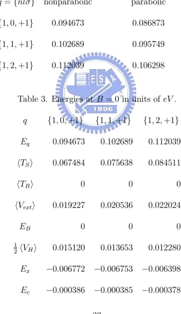
We next present the important effect of the band nonparabolicity. In Table 2, we observe that the energy differences between the parabolic and nonparabolic dispersion relations used in the Hamiltonian for zero magnetic field can be very significant since the magnitudes are comparable with that of the correlation ener-gies as shown in Table 3. For the parabolic dispersion case, the effective mass in (2.2) is taken as m = 0.024m0. In Tables 3 and 4, all energy components in (3.5) are separately presented to indicate the magnitudes of the energies from various effects. Here, the total ground-state energy E obtained via the KS eigenvalues εq is defined by [16]

E = N q Eq = N q εq− 1 2 e2 4π 0 (r) n(r)n(r ) |r − r | dr dr − σ V_xcσ(r)nσ(r)dr₋e c jp· Axcdr+Exc(n).

Table 2. Energies for the nonparabolic and parabolic approximation at B = 0 in units of eV . q =_{{nlσ} nonparabolic} parabolic {1, 0, +1} 0.094673 0.086873 {1, 1, +1} 0.102689 0.095749 {1, 2, +1} 0.112039 0.106298

Table 3. Energies at B = 0 in units of eV . q _{{1, 0, +1} {1, 1, +1} {1, 2, +1}} Eq 0.094673 0.102689 0.112039 TS 0.067484 0.075638 0.084511 TB 0 0 0 Vext 0.019227 0.020536 0.022024 EB 0 0 0 1 2 VH 0.015120 0.013653 0.012280 Ex −0.006772 −0.006753 −0.006398 Ec −0.000386 −0.000385 −0.000378

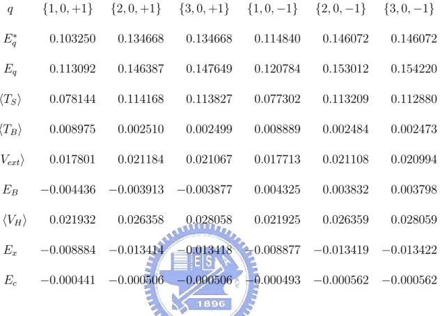
Table 4. Energies at B = 15 in units of eV .

Eq∗ are energies based on the single-particle Hamiltonian.

q _{{1, 0, +1} {2, 0, +1} {3, 0, +1} {1, 0, −1} {2, 0, −1} {3, 0, −1}} E∗ q 0.103250 0.134668 0.134668 0.114840 0.146072 0.146072 Eq 0.113092 0.146387 0.147649 0.120784 0.153012 0.154220 TS 0.078144 0.114168 0.113827 0.077302 0.113209 0.112880 TB 0.008975 0.002510 0.002499 0.008889 0.002484 0.002473 Vext 0.017801 0.021184 0.021067 0.017713 0.021108 0.020994 EB −0.004436 −0.003913 −0.003877 0.004325 0.003832 0.003798 1 2 VH 0.021932 0.026358 0.028058 0.021925 0.026359 0.028059 Ex −0.008884 −0.013414 −0.013418 −0.008877 −0.013419 −0.013422 Ec −0.000441 −0.000506 −0.000506 −0.000493 −0.000562 −0.000562

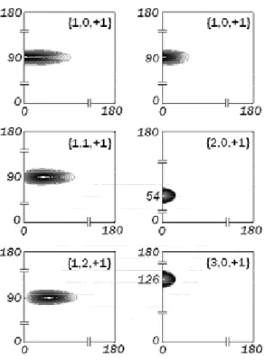
As stated above, our main concern for the present QDM model is to show the state change of the electrons under the influence of magnetic fields. The wave functions of the six electrons originally occupying the lowest 3 energy states with B = 0 as given in Table 3 are shown in the left panel of Fig. 4.2, which clearly illustrates that the electrons are residing in the central dot. For B = 15, we see that, corresponding to the lowest 6 energy states as given in Table 4, each one of these three dots contains two electrons for which their wave functions are shown in the right panel of Fig. 4.2. Note that three dimensional wave functions can be easily illustrated from these two dimensional wave functions via the formula (3.1).

Accuracy of the exchange energies can be verified by the ratio between the absolute values of 1₂ VH and Ex, which is about 2 for two-electron atoms [37]. It has been theoretically shown in [38] that this ratio is exactly equal to 2 for a two-electron model for which the xc energy and xc potential can be determined exactly in an external harmonic potential. From Tables 3 and 4, the ratio is approximately 2.

Finally, we remark that the essential physics of this study, namely the state change of electrons in QDM under the influence of magnetic field as such indicated by Fig. 4.2, can also be simulated by means of a much simpler model, e.g., the single-particle Hamiltonian with parabolic band structure (i.e., constant effective mass approximation). However, the numerics of the computed energies can be quite different from that of the present model as shown by the numbers in the second and third rows in Table 4. Moreover, we may obtain degenerate states such as_{{2, 0, +1} and {3, 0, +1} under the single-particle picture, which obviously} is incorrect. In addition to the effect of the model in use, the state change is significantly governed by the QDM dimensions as given in Fig. 1.1 so that we can attain the electronic behavior as shown in Fig. 4.2. These dimensions are also experimentally feasible [9].

Chapter 5

Concluding Remarks

A new mathematical model that incorporates the nonparabolic energy dispersion relation and realistic hard-wall finite confinement potential into the many-body Hamiltonian in the current spin density functional theory in 3D setting is pro-posed. It is used to study the electronic properties of a quantum dot molecule that consists of three vertically aligned semiconductor quantum dots (one large central dot and two smaller identical dots) under the influence of magnetic fields. A new Jacobi-Davidson method is given to solve the cubic eigenvalue problem resulting from finite difference approximation due to the nonparabolic nature of the effective mass. It is shown that the effect of band nonparabolicity can be very significant in the sense that the energy difference between the parabolic and non-parabolic cases is comparable with that of correlation energies in multielectronic system. Furthermore, we show that six electrons residing in the large central dot at zero magnetic field can be changed to such that each dot contains two electrons with some feasible magnetic field.

This thesis is intended to describe mathematical aspects of the model and to present preliminary physical results only on the Kohn-Sham orbitals and detailed

energy components with two different magnetic fields. Following this more realistic and accurate model, there are many interesting physical phenomena such as capac-itance, optical and transport properties, Wigner crystallization, Aharonov-Bohm oscillation, and quantum Hall effect can be further investigated for semiconduc-tor nanostructures in three dimensional space. In particular, with an additional electric control, we expect to have an energy selective mechanism to manipulating excitonic states of two closely spaced QDMs so that a strong coherent dipole-dipole coupling can be achieved and hence the F¨orster-Dexter resonant energy transfer between QDMs can be realized to motivate a new paradigm of Fermionic qubits for quantum computing in solid-state systems.

Part II

A Numerical Method for Exact

Diagonalization of Semiconductor

Chapter 6

Introduction

Exact diagonalization of many-body Hamiltonian is the most accurate and expen-sive method to study the electron dynamics and correlation in a semiconductor QD [44] [46] [47] [50] [51] [53] [28] [62]. Efficient methods such as the Hartree-Fock method and density functional approach are known to give substantial errors in energy, many-body wave function, spin-polarized states, and exchange-correlation potentials etc. [38] [46] [47] [50] [52].

Most of the theoretical models for QDs are based on 2D electron gas systems with parabolic infinite confinement potential, which are justifiable for calculat-ing scalculat-ingle-particle states, addition energy spectra, and many qualitatively new features of QDs. In fact, 2D models have turned out to be surprisingly rich and difficult [28]. However, the Coulomb interaction between electrons in QDs is three dimensional by nature and is the most important effect of many-body dynamics in QDs. It has been shown in [43] [54] that 2D models often lead to an inadequate description of the Coulomb interaction as a consequence of the overestimated car-rier localization. The 3D models are found to reproduce the experimental data for a large class of QD structures where simplified 2D models may fail [41] [45]

[48] [54].

There is another issue concerning the accuracy of QD models, namely, the effective-mass approximation (EMA) which allows us to model the conduction electrons in a QD as a decoupled interacting system with one-band effective mass from their environment that consists of millions of atoms in crystalline structure. This assumption makes numerous theoretical investigations possible within toler-able computing resources. Most of the existing models are based on the parabolic EMA. In [45], the QD model with nonparabolic EMA is shown to describe quan-titatively the capacitance-voltage and far-infrared measurement data. The model does estimate correctly the change in the effective mass due to the nonparabolic effect. Moreover, it is shown in [49] that the effect of band nonparabolicity can be very significant in the sense that the energy difference between the parabolic and nonparabolic cases is comparable with that of exchange energies in multielectronic system.

In addition to the computational complexity compounded greatly by the three dimensionality and the exact diagonalization, the nonparabolicity leads to nonlin-ear (cubic) eigenvalue problems with interior eigenvalues which are much harder to solve than that of linear eigenvalue problems [40] [25] [22] [56] [59] [24]. In this paper, we propose a numerical algorithm for exact diagonalization of the many-electron Hamiltonian of a disk-shaped 3D InAs/GaAs QD model with non-parabolic EMA. The algorithm consists of the advanced cubic Jacobi-Davidson

method developed in [25] [49], GMRES, a model reduction technique for both Schr¨odinger and Poisson equations, and a new numerical approach to the exact diagonalization.

The computation of all pair-wise Coulomb interactions is one of the limiting factors in ab initio electronic structure calculations [57]. Our model reduction technique is a consequence of cylindrical symmetry of the model. This technique allows us to calculate the Coulomb matrix elements within tolerable accuracy and computing times. The reduction technique is not meant for general purposes but for a test of our idea on the numerical exact diagonalization.

Since the states of a QD are localized in space, the plan-wave approach for 2D electron gas systems would require a very large number of Fourier components to define a localized state [43]. Another approach that has been developed to reduce the number of basis states is to construct the single-particle basis functions that are separable into an in-plane (parallel to the radial axis) and a perpendicular part. The Fock-Darwin states (associated with Laguerre polynomials) are a good choice for in-plane states because they are the eigenstates of parabolically confined electrons [42] [43] [53] [58]. The perpendicular, or subband, functions are deter-mined numerically by solving a 1D Hartree-Fock equation. The many-electron system is then solved by minimizing the total energy of all conduction electrons in the system in a function space spanned by a basis of multi-electron functions which are constructed as a direct antisymmetrized product of single-particle basis

functions. To achieve a convergence for a few-electron system, the size of the single-particle basis functions must be of the order of a million [53].

These approaches are not suitable for the model considered in this paper due to the hard-wall confinement potential and the nonparabolic EMA. We present here a fully numerical approach for the exact diagonalization of many-electron Hamiltonian. In our approach, the basis set of single-particle functions is ob-tained by solving the cubic eigenvalue problem resulting from a finite difference approximation of the single-electron QD model. The eigenvalue problem is solved by the block cubic Jacobi-Davidson method proposed in [49]. Since the single-particle spectrum depends on the hard-wall confinement potential which is finite, the size of the basis set will have an upper limit. The use of single-particle basis will thus reduce the computational cost without losing accuracy on the ground state energy of the whole system. Compared with other approaches, the trade-off of our approach is the solution of the cubic eigenvalue problem with the size of tens of thousands.

We briefly summarize the main results of our approach as follows. For a 4-electron QD with the hard-wall confinement potential taken as V0 = 0.77 eV (electron volts), we only need 12_{∼ 16 single-particle states to obtain a convergent} ground state energy within meV (milli-electron volts) accuracy. The computa-tional complexity of calculating all pair-wise Coulomb interactions is CNs

2 + Ns

where CNs

and 2, i.e., we need to solve the Poisson equation CNs

2 +Nstimes for this particular system.

The single-electron nonparabolic EMA model is given in the following chapter. Numerical methods for this model are briefly described in Chapter 8. We refer to [25] [24] for more mathematical details on the discretization of the model and the solution of the cubic eigenvalue problem. In Chapter 9, we introduce our exact diagonalization approach to the many-electron system. The special point to note is the construction of the basis set of multi-electron wave functions based on the single-electron functions. A simple example is given to illustrate the function sapce definition. In Chapter 10, we present the model reduction technique and numerical methods for calculating Coulomb matrix elements. An overall algorithm for the solution procedure of the many-electron system is summarized in this chapter as well. Numerical results are presented in Chapter 11. Finally, we make some concluding remarks in the last chapter.

Chapter 7

Single-Electron Model

Let the spatial domain of the QD model considered herein be a disk-shaped Ω = ΩInAs ∪ ΩGaAs ⊂ R3 as shown by a cross section of Ω in Fig. 7.1 where the InAs QD is embedded in the GaAs matrix whose dimensions are commensurable with that of [9] in which a transmission electron micrograph of a QD sample is illustrated. Within the nonparabolic EMA, the Hamiltonian for an electron in the QD is given by H0(r) = −h 2 2 ∇r 1 m(r,ε) ∇r+ Vc(r) (7.1) Vc(r) = ⎧ ⎪ ⎪ ⎪ ⎨ ⎪ ⎪ ⎪ ⎩ 0, in ΩInAs V0, in ΩGaAs (7.2) 1 m(r,ε) = p2 h2 2 ε + Eg(r)−Vc(r) + 1 ε + Eg(r)−Vc(r) + ∆(r) (7.3)

where_∇r stands for the spatial gradient, ε is the electron (unknown) energy, h is the reduced Planck constant, Eg(r) is the energy-band gap, ∆(r) is the spin-orbit splitting in the valence band, p is the momentum matrix element, and m0 is the free electron mass. Note particularly that the nonparabolic effective mass m(r,ε)

Figure 7.1: A cross section of a disk-shaped InAs quantum dot embedded in the GaAs matrix in real space dimensions in nano meters that are used in numerical implementation.

depends on both position and electron energy and that the hard-wall confinement potential Vc is induced by a discontinuity of conduction-band edges of InAs and GaAs. All numerical values of the parameters used in this paper are listed in Table 1 which also includes the corresponding units and cited references.

Chapter 8

Numerical Methods for Single

Electron Wave Functions

To obtain the states of the many-body system, we begin by solving the single particle problem

H0Φ = εΦ. (8.1)

Due to cylindrical symmetry, the envelope wave functions Φ (r) of this problem can be expressed as

Φq(r) = e−ilθφq(r, z) , q ≡ {nl} , (8.2)

where n is the principal quantum number, and l = 0,_{±1, ±2, · · · is the quantum} number of the projection of angular momentum onto the z-axis. Eq. (8.1) can then be reduced to a 2D problem in the (r, z) coordinates as

H0φq(r, z) = εqφq(r, z) , (8.3)

H0 =− h2 2m(r, z, εq) ∂2 ∂r2 + 1 r ∂ ∂r − l2 r2 + ∂2 ∂z2 + Vc(r, z) (8.4) In 2D setting, the solution domain for (8.3) is again expressed by the same notation as that of 3D, that is, Ω = ΩInAs∩ ΩGaAs ⊂ R2. We choose the do-main ΩGaAs sufficiently large so that the wave function is negligibly small at the boundary of ΩGaAs. By symmetry, the domain Ω can be reduced to Ω = {(r, z) : 0 ≤ r ≤ rmax, 0≤ z ≤ zmax} for sufficiently large rmax > 0 and zmax > 0 as shown in Fig. 7.1.

Since we are dealing with the hard-wall confinement potential, the interface conditions of the wave function in (8.3) has to be specifically imposed, namely,

⎧ ⎪ ⎪ ⎪ ⎨ ⎪ ⎪ ⎪ ⎩ 1 m(r,z,εq)∇φq(r, z)· n _Γ− = 1 m(r,z,εq)∇φq(r, z)· n_Γ+, φq(r, z)|_Γ− = φq(r, z)|_Γ+, (8.5)

where Γ denotes the interface between two materials, i.e., Γ = ΩInAs∩ ΩGaAs, n is an outward normal unit vector on the boundary of ΩInAs, and Γ− and Γ+are the sets of limiting points to the curve Γ from the interior and the exterior of ΩInAs, respectively. The momentum operator_{∇ is similarly defined for the 2D case. The} boundary conditions for (8.4) are

⎧ ⎪ ⎪ ⎪ ⎨ ⎪ ⎪ ⎪ ⎩ ∂φq(r,z) ∂r _W = 0, φq(r, z) = 0, on S, E, N, (8.6)

the domain Ω. Note that on the west side of the boundary the values of the wave function are taken to be the same for satisfying the continuity condition across W . In actual implementation this condition is replaced by taking the values of the two horizontal grid points adjacent to W as the same. Moreover, to avoid numerical over-flow due to the term 1/r in (8.4), we do not define unknowns at the grid points on W .

We then use the standard finite difference method to approximate the model problem. Since the mass in (7.3) is energy dependent, Eqs. (8.3), (8.5), and (8.6) result in a system of cubic eigenvalue equations

A0+ λA1+ λ2A2+ λ3A3 x= 0, (8.7)

where the unknown eigenpair (λ, x) is an approximate solution of (εq, φq) for some q at grid points. Starting from the Schr¨odinger equation, finite difference discretization, to the coefficient matrices A0, A1, A2, and A3, a detailed derivation of the same cubic eigenvalue system is given in Appendix (or[24]). Several Jacobi-Davidson methods are proposed and compared in [25] for solving this type of eigenvalue problems.

Chapter 9

Many-Electron Model

To describe a system of N electrons in a QD under the influence of the Coulomb interaction, we write the total Hamiltonian H as a sum of single-particle operators Hi and two-body operators Vij in the envelope-function approximation as

H = N i=1 Hi+ 1 2 _i=jVij (9.1) Hi = H0(ri) (9.2) Vij = VC(ri, rj) = e2 4π 0 (ri) 1 |ri− rj| (9.3)

where the single-electron Hamiltonian H0(ri) is defined as (7.1) for the ith electron and e is the proton charge. For the sake of simplicity in exposition, the mutual interaction between the electrons in the system is taken to be purely Coulombic. From single-particle picture to many-particle picture for QDs, we follow the theoretical framework developed by Pietil¨ainen and Chakraborty in [53]. The approximate eigen-pairs (εq, φq) form a single-particle basis set

From this set, a basis BN for N interacting electrons in a QD can be constructed as a direct antisymmetrized product of B of the form

BN =A N

j=1

B =_{|Qi : i = 1, 2,· · · , Nm} , (9.5)

where Ns is the total number of computed single-particle states, A denotes the antisymmetrization operator, and Nm = CNNs. More specificly, the many-body basis functions _|Qi are Slater determinants defined as

|Qi = A [|qi1 ⊗ |qi2 · · · ⊗ |qiN ] = √1 N ! Φq_i1 (r1) Φq_i2 (r1) · · · Φq_iN (r1) Φq_i1 (r2) Φq_i2 (r2) · · · Φq_iN (r2) .. . ... ... ... Φq_i1(rN) Φq_i2(rN) · · · Φq_iN(rN) . (9.6)

The states of the interacting system are then expressed by the superposition of the non-interacting states (9.5) as

|Ψ = Nm

i=1

ci|Qi , (9.7)

where the unknown coefficients ci are sought by minimizing the energy functional

Ψ_{|H| Ψ} (9.8)

Ψ_{|Ψ = 1.} (9.9)

An Example

We now illustrate the above formalism by considering a simple case as follows:

N = 2, Ns = 3 (9.10) B = _{|Φq : q = 1, 2, 3} (9.11) Nm = C23 = 3! 2!1! = 3 (9.12) B2 = A 2 q=1 B =_{|Qi : i = 1, 2,· · · , Nm} (9.13) |Q1 = |q1; q2 = 1 √ 2 Φ1(r1) Φ2(r1) Φ1(r2) Φ2(r2) (9.14) |Q2 = |q1; q3 = 1 √ 2 Φ1(r1) Φ3(r1) Φ1(r2) Φ3(r2) (9.15) |Q3 = |q2; q3 = 1 √ 2 Φ2(r1) Φ3(r1) Φ2(r2) Φ3(r2) (9.16) |Ψ = 3 j=1 cj|Qj (9.17) Ψ_{|H| Ψ} = dr1dr2 3 i=1 cj|Qj ∗ H 3 i=1 cj|Qj (9.18) Ψ_|Ψ = dr1dr2|Ψ (r1, r2)| 2 = 1 (9.19)

Using the method of Lagrange multipliers, the minimization of (9.8) subject to (9.9) leads to ∂ ∂ci { Ψ |H| Ψ − λ Ψ|Ψ } = 0, i = 1, 2, 3, (9.20) ∂ ∂ci Ψ_{|H| Ψ} = dr1dr2|Qi ∗H ⎛ ⎝ 3 j=1 cj|Qj ⎞ ⎠ + dr1dr2 ⎛ ⎝ 3 j=1 cj|Qj ∗ ⎞ ⎠H_|Qi (9.21) ∂ ∂ci λ Ψ_{|Ψ = 2λ} 3 j=1 cj dr1dr2|Qi ∗|Qj (9.22) Hij = Qi|H| Qj = Qi H1+ H2+ 1 2V12 Qj (9.23) Q2|H1| Q3 = dr1dr2Q∗2H1Q3 (9.24) = 1 2 dr1dr2[Φ ∗ 1(r1) Φ∗3(r2)− Φ∗1(r2) Φ∗3(r1)] H1 [Φ2(r1) Φ3(r2)− Φ2(r2) Φ3(r1)] (9.25) = 1 2 dr1dr2[Φ ∗ 1(r1) Φ∗3(r2)− Φ∗1(r2) Φ∗3(r1)] [Φ3(r2) H1Φ2(r1)− Φ2(r2) H1Φ3(r1)] (9.26) Q2|H2| Q3 = 1 2 dr1dr2[Φ ∗ 1(r1) Φ∗3(r2)− Φ∗1(r2) Φ∗3(r1)] [Φ2(r1) H2Φ3(r2)− Φ3(r1) H2Φ2(r2)] (9.27)

Q2 1 2V12 Q3 = 1 4 dr1dr2[Φ ∗ 1(r1) Φ∗3(r2)− Φ∗1(r2) Φ∗3(r1)] e2 4π 0 (r1) 1 |r1− r2| [Φ2(r1) Φ3(r2)− Φ2(r2) Φ3(r1)] (9.28) ⎡ ⎢ ⎢ ⎢ ⎢ ⎢ ⎢ ⎢ ⎢ ⎣ H11 H12 H13 H21 H22 H23 H31 H32 H33 ⎤ ⎥ ⎥ ⎥ ⎥ ⎥ ⎥ ⎥ ⎥ ⎦ ⎡ ⎢ ⎢ ⎢ ⎢ ⎢ ⎢ ⎢ ⎢ ⎣ c1 c2 c3 ⎤ ⎥ ⎥ ⎥ ⎥ ⎥ ⎥ ⎥ ⎥ ⎦ = λ ⎡ ⎢ ⎢ ⎢ ⎢ ⎢ ⎢ ⎢ ⎢ ⎣ c1 c2 c3 ⎤ ⎥ ⎥ ⎥ ⎥ ⎥ ⎥ ⎥ ⎥ ⎦ (9.29)

Therefore, the total energy of N electrons in the QD can be obtained by diagonalizing the linear eigenvalue problem

Nm

j=1

(Hij− λδij) cj = 0, (9.30)

where the eigenvectors c = [c1 c2 · · · cNm]

T

are the desired expansion coefficients and the eigenvalues λ the corresponding energies of the interacting system.

The finite confinement potential leads to a finite number of localized states as well as to energetically higher delocalized states. When the influence of the delo-calized states on the discrete QD spectrum is neglected, the eigenvalue problem (9.30) has a finite dimension and can be solved without further approximations. The most computationally expensive part is the calculation of the Coulomb ma-trix elements (9.28) whereas the other parts (9.26) and (9.27) can be directly calculated from (8.7) or equivalently from (8.3).

Obviously, the computational complexity is essentially determined by Nswhich in turn is limited by the confinement potential strength V0 in (7.2). This is the

main difference between our approach and the others such as those in [43] [42] [53] [58] where the size of the single-particle basis (analytical) functions must be of the order of a million owing to the approximation by means of either the 2D electron gas modeling or the subband structure. We also note that the choice of analytical functions, e.g. Laguerre polynomials, for the single-particle basis is not feasible for our model because of the finite and local nature of the confinement potential V0 and the nonlinear dependence of the effective mass m(r,ε) on both position and electron energy. In fact, the evaluation of Coulomb matrix elements by using Laguerre polynomials is numerically highly unstable owing to large terms of alternating sign in the polynomail [53].

Our approach is convergent, stable, and robust (see below). However, the trade-off of our approach is the solution of the cubic eigenvalue problem (8.7) with the size of tens of thousands.

Chapter 10

Numerical Methods for Coulomb

Matrix Elements

Since the basis states _|Qi have been constructed by diagonalizing H0, we are left to compute the Coulomb matrix elements defined by the two-body operator VC of (9.3) as 12_|VC|34 = dr drΦ∗1(r)Φ∗2(r ) e2 4π 0 (r) 1 |r − r |Φ3(r)Φ4(r ) (10.1) = dr dreil1θ_φ 1(r, z) e−il3θφ3(r, z) e2 4π 0 (r) 1 |r − r | eil2θ _φ 2 r , z e−il4θ φ4 r , z , (10.2) for any arbitrary states Φi(r), i = 1, 2, 3, 4, representing four-center two-electron repulsion integrals. For real space approximation, we define a potential-like func-tion V24(r) as V24(r) = e2 4π 0 (r) eil24θ _φ 24 r , z |r − r | dr (10.3)

where l24= l2− l4 and φ24 r , z = φ2 r , z φ4 r , z . This function can then be cast into a Poisson equation

∇ · (r)∇V24(r) =− e2 4π 0

eil24θ_φ

24(r, z) . (10.4)

By cylindrical symmetry, this equation can be written as

∂2 ∂r2 + 1 r ∂ ∂r + 1 r2 ∂2 ∂θ2 + ∂2 ∂z2 V24(r, θ, z) = e il24θ_{f (r, z), (10.5)} f (r, z) = ₋ e 2 4π 0 i φ24(r, z) , for i = 1 or 2, (10.6)

where 1 = InAs if (r, z)∈ ΩInAs and 2 = GaAs if (r, z)∈ ΩGaAs. By using the method of separating variables and substituting a solution of the form

V24(r, θ, z) = V24(r, z) V24(θ) (10.7) into (10.5), we have e−il24θ_V 24(θ) ∂2 ∂r2 + 1 r ∂ ∂r + ∂2 ∂z2 V24(r, z) +e−il24θ_V 24(r, z) 1 r2 ∂2_V 24(θ) ∂θ2 = f (r, z) or e−il24θ_V 24(θ)r2 V24(r, z) ∂2 ∂r2 + 1 r ∂ ∂r + ∂2 ∂z2 V24(r, z)

+e−il24θ∂ 2_V 24(θ) ∂θ2 = r2 V24(r, z) f (r, z). (10.8)

Obviously, the function V24p(θ) = eil24θ is a particular solution of (10.8) if we view (10.8) as a second order nonhomogeneous ordinary differential equation with respect to θ provided that there exists a function V24p (r, z) satisfing the 2D Poisson equation ∂2 ∂r2 + 1 r ∂ ∂r + ∂2 ∂z2 − l2 24 r2 V p 24(r, z) = f (r, z). (10.9) This implies that V₂₄p (r, θ, z) = V₂₄p (r, z) V₂₄p(θ) is a particular solution of (10.5). The general solution of the corresponding homogeneous equation is thus eikθ_Vh

24(r, z) such that Vh

24(r, z) satisfies the Laplace equation

∂2 ∂r2 + 1 r ∂ ∂r + ∂2 ∂z2 − k2 r2 V h 24(r, z) = 0 (10.10) for any integer k. The general solution of the nonhomogeneous equation (10.8) (or (10.5)) is therefore of the form

k

eikθV24h(r, z) + V p

24(r, z) . (10.11) In 2D setting, we also have interface conditions for Poisson’s problem, namely,

⎧ ⎪ ⎪ ⎪ ⎨ ⎪ ⎪ ⎪ ⎩ (r, z)_∇V24p (r, z)· n|Γ− = (r, z)∇V p 24(r, z)· n|Γ+, V24(r, z)|Γ− = V24(r, z)|Γ+. (10.12)

Similarly, the boundary conditions for (10.4) are ⎧ ⎪ ⎪ ⎪ ⎨ ⎪ ⎪ ⎪ ⎩ ∂V₂₄p(r,z) ∂r _W = 0, V₂₄p (r, z) = 0, on S, E, N. (10.13)

By imposing these boundary conditions to the general solution (10.11), we deduce that the particular solution V24p (r, z) is in fact a general solution of (10.8) and thus of (10.5), i.e., Vh

24(r, z) = 0. This implies that V24(r, θ, z) = eil24θV24p (r, z) is a general solution of (10.4). Consequently, we have 12_|Vc|34 = Φ∗1(r)Φ3(r)eil24θV24p (r, z) dr (10.14) = 2π 0 e i(l13−l42)θ_{dθ φ} 13(r, z) V p 24(r, z) rdrdz (10.15) = 2πδl13l42 φ13(r, z) V p 24(r, z) rdrdz (10.16)

where the computation of the 3D Coulomb matrix element (10.1) is reduced to solving the 2D problem (10.9).

Again the finite difference method is used for solving the Poisson problem (10.9), (10.12), and (10.13). This leads to a system of algebraic equations

Ax = b, (10.17)

where now the unknown vector x corresponds to the approximate values of V24p (r, z) at the grid points.

We summarize the above methods for studying the electronic properties of few interacting electrons confined in a QD via exact diagonalization as follows.

An Exact Diagonalization Algorithm:

(0) Set the number of electrons N and the number of single-particle states Ns. The number of many-body basis functions Nm = CNNs.

(1) Solve the single-particle problem (8.1) in discrete form (8.7) for Ns basis functions by means of the cubic Jacobi-Davidson method for some principal quantum numbers n and angular momentum quantum numbers l (8.2) which are determined by Ns.

(2) Use the Ns basis functions to construct Nm Slater determinants (9.6).

(3) Evaluate Coulomb matrix elements (10.16) by solving the Poisson problem (10.9), (10.12), (10.13) in discrete form (10.17) via GMRES [34].

(4) Solve the eigenvalue problem (9.30) for the lowest eigenvalue (ground state energy) and the corresponding eigenvector of the N -electron system by using the QR algorithm [36].

Chapter 11

Numerical Results

Since Coulomb interaction has a long-range tail, the computational domain must be sufficiently large. We first determine the size of the domain in Fig. 7.1 by inspecting the rate of change of the ground state energy with respect to rmax = zmax for a 2-electron system with Ns = 8. As shown in Fig. 11.1, the change of the ground state energy around rmax = 100 nm and beyond is relatively small. The following numerical results are thus based on the domain with rmax = 100 nm. On the (100,100) nm2 _{domain, we set 151 nonuniform grid points [24] along} each direction for the finite difference approximation.

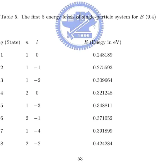
In order to have a sufficiently large basis set B (9.4), it is necessary to solve (8.4) with various l from 0 to _{−4. Some smallest positive real eigenvalues and} their associated eigenvectors of (8.7) are computed for each l. Some of the first low-lying energy levels of the single-electron system are shown in Table 5. If all these states are taken to be the basis of B, then Ns= 8.

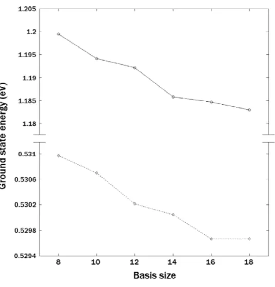
The ground state energies of 2 and 4 electrons with various basis numbers Ns are shown in Table 6 and plotted in Fig. 11.2. It is clear that the many-electron QD can be modeled to a very good precision with the energy down to the order of

milli-electron volts (meV ) by using just few tens of single-partical basis functions. The convergence behavior of the ground state energy with respect to the basis size Ns of our approach is also clearly demonstrated by the figure.

The computational complexity increases quadratically with Ns. For example, for the case of Ns = 18, we need to solve the Poisson problem, i.e., the linear system (10.17) C18

2 + 18 = 171 times for Coulomb matrix elements. Nevertheless, all of our numerical methods for solving the systems (8.7), (9.30), and (10.17) are stable and convergent.

Table 5. The first 8 energy levels of single-particle system for B (9.4).

q (State) n l E (Enegy in eV)

1 1 0 0.248189 2 1 ₋₁ 0.275593 3 1 ₋₂ 0.309664 4 2 0 0.321248 5 1 ₋₃ 0.348811 6 2 ₋₁ 0.371052 7 1 ₋₄ 0.391899 8 2 ₋₂ 0.424284

Table 6. Ground state energies of N -electron system with respect to Ns. N Ns λ (eV) 2 12 0.530213 2 14 0.530046 2 16 0.529667 2 18 0.529667 4 12 1.192199 4 14 1.185846 4 16 1.184708 4 18 1.182987

Figure 11.1: The effect of the domain size on the ground state energy of two-electron system with the basis size Ns = 8.

Figure 11.2: The ground state energies of two- and four-electron QDs as a function of the basis size Ns from 8 to 18.

Chapter 12

Concluding Remarks

We have presented a numerical approach to the exact diagonalization of many-electron Hamiltonian in semiconductor quantum dots within the nonparabolic effective mass and realistic 3D confinement potential approximation. The many-electron wave function is expanded in a basis of Slater determinants constructed from numerical wave functions of the single-particle Hamiltonian system. The finite confinement potential implies the boundedness of the single-particle states and thus the finite dimensionality of the function space of many-electron wave functions.

It has been shown that we only need about Ns = 18 single-particle states to obtain a convergent ground state energy of a 4-electron system within meV (milli-electron volts) accuracy. The complexity for calculating all pair-wise Coulomb interactions is O (N2

s). All numerical methods used in our algorithm are stable and convergent. The approach proposed here is whereby robust for more general, realistic, and accurate models of nanoscale semiconductor heterostructures.

Chapter 13

Conclusions

This thesis studies two methods in calculating the electronic energy spectrum of the many-electron Hamiltonian: the current spin density functional theory and the exact diagonalization technique. The main characteristics and results of our models are summarized as follows:

Part I. QDM based on the current spin density functional theory.

(1) We propose a new mathematical model that incorporates the nonparabolic energy dispersion relation and realistic hard-wall finite confinement poten-tial into the many-body Hamiltonian in the current spin density functional theory in 3D setting.

(2) A QDM that consists of three vertically aligned semiconductor quantum dots (one large central dot and two smaller identical dots) under the influence of magnetic fields is used in numerical implementation.

(3) Instead of using deflation scheme in the JD solver [25], a new JD method that allows us to compute several eigenpairs simultaneously and to have a block implementation of the search subspaces is given to solve the cubic

eigenvalue problem resulting from finite difference approximation due to the nonparabolic nature of the effective mass.

(4) From Tables 3 and 4, the accuracy of the exchange energies is verified by the ratio between the absolute values of 1₂ VH and Ex. This ratio, in accordance with the literature [37] [38], is approximately 2.

(5) In Fig. 4.2, it is shown that six electrons residing in the large central dot at zero magnetic field can be changed to such that each dot contains two electrons with some feasible magnetic field. The F¨orster energy transfer may therefore be generated by two individual QDMs. This may motivate a new paradigm of Fermionic qubits for quantum computing in solid-state systems.

Part II. A numerical method for exact diagonalization of semiconductor QD model.

(1) In this approach, the QD model used is based on realistic 3D finite hard-wall confinement potential and nonparabolic EMA that render analytical basis functions such as Laguerre polynomials inaccessible for the numerical treatment of this kind of models.

(2) The many-electron wave function is expanded in a basis of Slater deter-minants constructed from numerical wave functions of the single-electron Hamiltonian with the nonparabolic EMA.

(3) The cubic eigenvalue problems resulting from the calculations of single-electron basis states are solved by using JD method described as above.

(4) As shown in Fig. 11.1, the long-range character of the Coulomb interaction has a profound influence on the ground state energy. Thus, the finite differ-ence approximations of the Schr¨odinger equations and the Poisson equations are performed on a rather large domain with nonuniform mesh.

(5) From Fig. 11.2, it is evident that a good convergence can be achieved by means of a few single-electron basis states.

Appendix

In this appendix, a derivation of the resulting cubic eigenvalue problem (3.20) (or(8.7)) from the finite difference discretization is briefly sketched. For simplicity, we only consider the case in which nonlinear terms are neglected, that is

Hφ (r, z) = εφ (r, z) , (A.1)

where the Hamiltonian is defined by

H = TS+ TB+ Vext+ VB, (A.2) TS(r, z) = − h2 2m(r, z, ε) ∂2 ∂r2 + 1 r ∂ ∂r − l2 r2 + ∂2 ∂z2 , (A.3) TB(r, z) = e2_B2_r2 8m(r, z, ε) + heBl 2m(r, z, ε), (A.4) Vext(r, z) = ⎧ ⎪ ⎪ ⎪ ⎨ ⎪ ⎪ ⎪ ⎩ 0, in ΩInAs V0, in ΩGaAs. , (A.5) VB(r, z) = σ 1 2g(r, z,ε)µBB. (A.6)

M1 ≡ Eg(r, z)−Vext(r, z), (A.7) M2 ≡ Eg(r, z)−Vext(r, z) + ∆(r, z). (A.8)

Then, the effective mass and the Land´e factor can be rewritten as

1 m(r, z,ε) = p2 h2 3ε + M1+ 2M2 (ε + M1)× (ε + M2) , (A.9) g(r, z,ε) = 2 [h 2 × (ε + M1)× (ε + M2)]− (m0p2∆(r, z)) h2_{× (ε + M} 1)× (ε + M2) . (A.10)

By using the standard central finite difference method and substituting the ex-pressions of the effective mass and the Land´e factor into (A.1), we have

0 = ₋ p

2_{(3ε + M}

1+ 2M2) 2 (ε + M1)× (ε + M2)

φi,j+1− 2φi,j+ φi,j−1 (∆r)2 + 1 rj φi,j+1− φi,j−1 2∆r −l 2 r2 j φi,j +

φi+1,j − 2φi,j + φi−1,j (∆z)2 + e 2_B2_r2 jp2(3ε + M1+ 2M2) 8h2_{(ε + M} 1)× (ε + M2) +heBlp 2_{(3ε + M} 1+ 2M2) 2h2_{(ε + M} 1)× (ε + M2) + Vext(rj, zi) +σµBB h2 × (ε + M1)× (ε + M2)− (m0p2∆(rj,zi)) h2_{× (ε + M} 1)× (ε + M2) − ε φ i,j. (A.11)

where ∆r and ∆z are mesh lengths in r and z directions, respectively, and φi,jis an approximated value of function φ at the grid point (rj, zi) for i = 1, . . . , n, and j = 1, . . . , n. Here, the index n denotes the grid point number. In Part I, all numerical