多重假設測試於訊號偵測之應用

國 立 交 通 大 學

電子工程學系 電子研究所碩士班

碩

士

論

文

多重假設測試於訊號偵測之應用

Signal Detection Using A Multiple Hypothesis Test

研 究 生：林宗熹

指導教授：鍾佩蓉博士

林大衛博士

多重假設測試於訊號處理之應用

Signal Detection Using A Multiple Hypothesis Test

研究生: 林宗熹

Student:

John-Si

Lin

指導教授: 鍾佩蓉博士 Advisor:

Dr. P. J. Chung

林大衛博士

Dr. David W. Lin

國 立 交 通 大 學

電子工程學系 電子研究所碩士班

碩士論文

A Thesis

Submitted to Department of Electronics Engineering & Institute of Electronics College of Electrical and Computer Engineering

National Chiao Tung University in Partial Fulfillment of Requirements

for the Degree of Master of Science

in

Electronics Engineering June 2006

Hsinchu, Taiwan, Republic of China

多重假設測試於訊號偵測之應用

研究生：林宗熹 指導教授： 鍾佩蓉 博士

林大衛 博士

國立交通大學

電子工程學系 電子研究所碩士班

摘要

在多樣化的應用裡，訊號源的檢測估計在理論上一直佔有很大的研究空間，隨著 不同的應用，陣列感應器訊號處理已發展成一個活躍的研究領域。許多的技術已經發 展出針對現實上不同問題的解決之道，例如雷達或利用聲納探測出訊號源的位置。 MUSIC 與 ESPRIT 是早期用於偵測訊號來源方向的方法。1970 年代，AIC 與 MDL 準則是為了選擇模型規模而發展出得兩種不同方法。很多方法在過去幾年當中，已經 發展出針對不同的情境而有不同的演算法，例如在同步訊號源或感應器數目非常少的 情況下。本論文的目的即是藉由結合統計的處理方法，使新的演算法達到更好的成效。 本論文的方向始自於多重假設測試在訊號處理上的應用。Bonferroni 程序目的在 於控制在即時考量下，同類比較測試時導致第一型錯誤的機率。如此一般的同類型錯 誤率得出的結果是趨於保守的。隨著統計處理的發展，多重假設測試的錯誤率可以控 制 在 某 一 個 信 心 水 準 之 下 ， 尤 其 在 某 些 特 定 的 程 序 比 較 中 可 以 控 制 的 更 低 。 Benjamini-Hochberg 程序展現出一種更加有效用的方法來達到更好的效果，而且保持 錯誤率在一定的信心水準之下。本論文將在介紹這一個程序的流程與效用，並且應用 於訊號偵測的領堿，創新並檢驗是否能達到更好的效用。

Signal Detection Using A Multiple Hypothesis Test

Student: John-Si Lin Advisor: Dr. P. J. Chung

Dr. David W. Lin

Department of Electronics Engineering & Institute of Electronics

College of Electrical and Computer Engineering

National Chiao Tung University

Abstract

Estimation problems in theoretical have been of great research interest in a great variety of applications. With application variation, sensor array signal processing developed as an active area of research. Many techniques have shown solutions for several real-world problems, such as source localization in radar and sonar. MUSIC and ESPRIT are parametric-based methods for detecting the locations of sources. AIC and MDL criteria are two kinds of approaches for model selection developed around 1970s. Many approaches in different situations, such as coherent signals or small number of sensors, were developed for the past years. Our goal is attempt to improve the performance by combining statistics processing.

Our idea comes from the multiple test which were tested in strong sense. The Bonferroni procedure controls the probability of committing any type I error in families of comparisons under simultaneous consideration. This control of familywise error rate results in conservative effects. With statistics development, the error rate of multiple hypotheses tests can be controlled under a certain level, especially lower in some of the procedure points. The Benjamini-Hochberg procedure shows a more powerful procedure to reach better performance and still maintain error rate under certain significance level. This work will introduce the controlling procedure and show the result with combing source detection problem.

誌謝

這篇論文能夠順利完成，最要感謝的人是我的指導教授 鍾佩蓉 博士。在這 二年的研究生涯中，不論是學業上或生活上，處處感受到老師的用心，讓我能在 遇到瓶頸時，有勇氣與毅力繼續前進。感謝另一位共同指導老師 林大衛 博士， 除了豐富的學識和研究，老師親切、認真的待人處事態度，也是我景仰、學習的 目標。 另外要感謝的，是楊華龍學長。感謝學長撥冗提供我了許多研究方面相關的 疑問以及研究進行的方向。 感謝通訊電子與訊號處理實驗室(commlab)，提供了充足的軟硬體資源，讓 我在研究中不虞匱乏。感謝實驗室的同學，平日一起唸書，一起討論，也一起分 享喜悅，讓我的研究生涯充滿歡樂又有所成長。 感謝我所有的親愛的同學與朋友，蕙君、俊甫、元銘、耕毅、國和、士浤、 紹茗、信豪、軒榮，在我口試前夕生病住院那幾天前來照顧與打氣，以及陪我度 過二年的研究所生活。 最後，要感謝的是我的家人，他們的支持讓我能夠心無旁騖的從事研究工作。 謝謝所有幫助過我、陪我走過這一段歲月的師長、同儕與家人。謝謝！ 誌於 2006.6 風城交大 宗熹

Contents

1 Introduction 1

2 Background and Signal Model 4

2.1 System and Propagating Waves . . . 4

2.2 Wavenumber-Frequency Space . . . 10

2.3 Random Fields . . . 11

2.3.1 Stationary Random Fields . . . 11

2.3.2 Correlation Matrices of Sensor Outputs . . . 13

2.4 Assumptions on Signal and Noise . . . 15

3 Signal Detection Using a Multiple Hypothesis Test 19 3.1 Eigenanalysis Methods . . . 19

3.1.1 Eigenanalysis . . . 19

3.1.2 Signal and Noise Subspaces . . . 20

3.2 Multiple Hypothesis Test . . . 22

3.2.1 Multiple Hypothesis . . . 24

3.2.3 Control of the global level . . . 31

4 Simulation 39

5 Conclusion and Future Work 45

Appendix A: Neyman Pearson Lemma 48

List of Figures

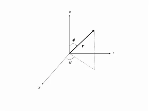
2.1 The spherical coordinate system, where θ is azimuth, φ elevation, and r

dis-tance from origin. . . 5

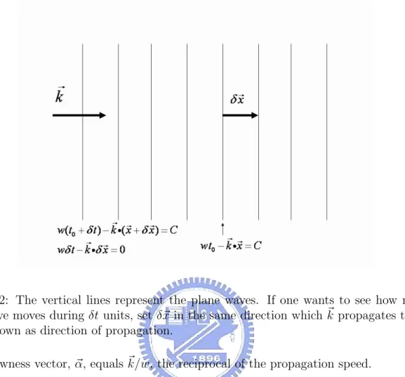
2.2 The vertical lines represent the plane waves. If one wants to see how much a plane wave moves during δt units, set δ~x in the same direction which ~k propagates towards and is known as direction of propagation. . . 8

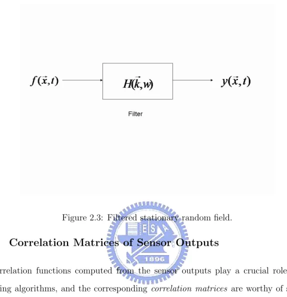
2.3 Filtered stationary random field. . . 13

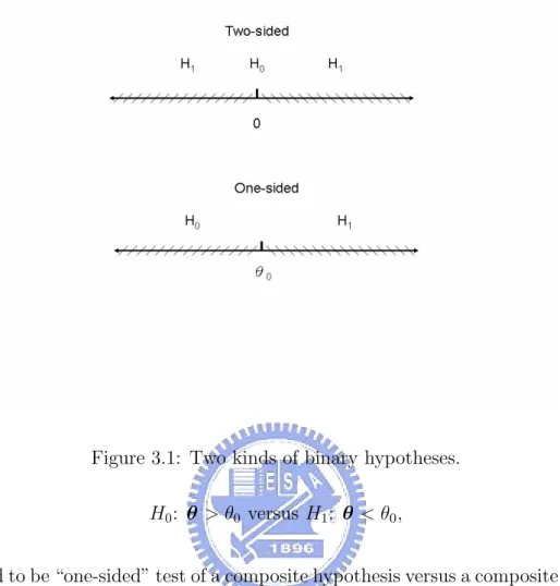
3.1 Two kinds of binary hypotheses. . . 26

3.2 A typical power curve. . . 28

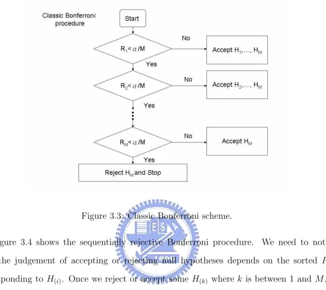
3.3 Classic Bonferroni scheme. . . 34

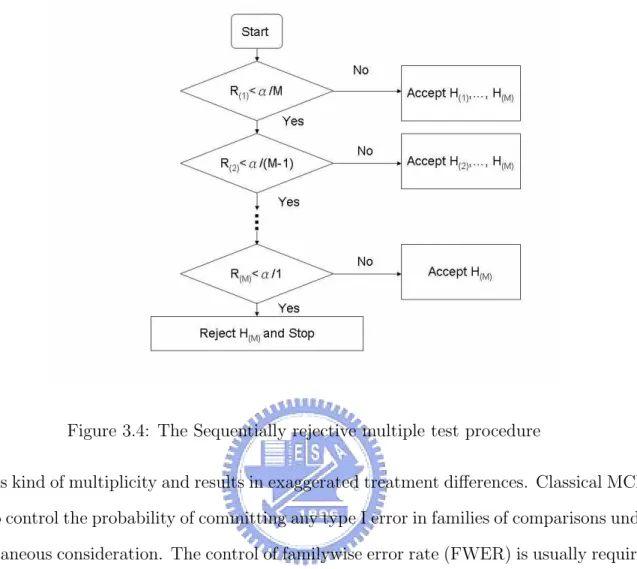
3.4 The Sequentially rejective multiple test procedure . . . 35

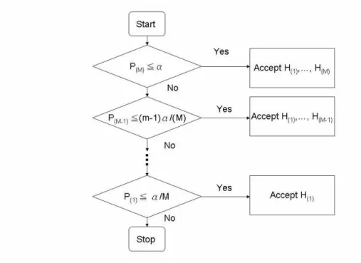
3.5 The Benjamini Hochberg procedure. . . 38

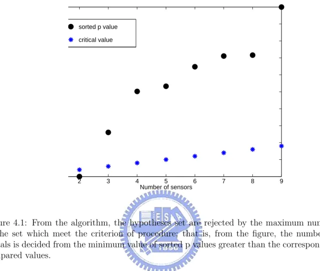
4.1 From the algorithm, the hypotheses set are rejected by the maximum number of the set which meet the criterion of procedure; that is, from the figure, the number of signals is decided from the minimum value of sorted p values greater than the corresponding compared values. . . 40

4.3 Three sources are generated from 10o_{, 50}o _{and 80}o _{direction of arrival,}

respec-tively. The array consists 7 sensors with snapshots T = 50. α = 0.01 and SNR = [−5:0.5:0] dB . . . . 42 4.4 Two sources are located closely from 20o_{, 30}o _{direction of arrival, respectively.}

The upper simulation contains 10 sensors and the underside one contains 5 only. SNR = [−6:0.5:3] dB, Other parameters remain unchanged. . . . 43 4.5 Under the same scenario as Fig. 4.4, the only difference is that the sources are

from 40o _{and 50}o_{. It can be observed that if the difference of DOA (Degree}

Of Arrivals) does not change, the result almost remains unchanged. . . 44 1 Neyman-Pearson Criterion representation. The ratio of shadowed area to

whole area of fθ0(x) is α, the size of test. . . . 49

Chapter 1

Introduction

Estimation problems in theoretical have been of great research interest in a great variety of applications. With application variation, sensor array signal processing developed as an ac-tive area of research. Many techniques have shown solutions for several real-world problems, such as source localization in radar and sonar. Subspace-Based methods, such as MUltiple SIgnal Classification (MUSIC), was indeed originally presented as a DOA estimator. Estima-tion of Signal Parameters Via RotaEstima-tional Invariance Techniques (ESPRIT) is an algorithm that dramatically reduces theses computation and storage cost. It is more robust with re-spect to array imperfections than MUSIC; however, both of them are not the techniques we focus on in this work because they do not involve the concepts of multiple hypotheses test.

The parametric methods of signal processing require often not only the estimation of a vector of real-valued parameters but also the selection of one ore several integer-valued para-meters that are equally important for the specification of a data model. For example, orders of an autoregressive moving average model, number of sinusoidal components in a sinusoids-in-noise signal, number of source signals impinging on a sensor array are theses kind of cases. The integer-valued parameters determine the dimension of the parameter vector of the data model, and thy must be estimated from the data. The task of selecting the above mentioned integer parameters is known as model order selection. Akaike Information Criterion (AIC)

and Minimum Description Length (MDL) are two kind of information Theoretic approaches developed around 1970s for such a problem. The approach MDL is consistent, whereas the AIC is not. The definition of consistency means that when the sample size increases to in-finity, estimated probability goes to one. The advantage of information theoretic criterion is that it does not need any subjective judgment to detect the number of sources. It determined as the value for which the AIC or MDL criterion is minimized. However, the drawback of these methods is failure in the presence of coherent signals. Many approaches in different situations, such as coherent signals or small number of sensors, were developed for the past years. Our goal is attempt to improve the performance by combining statistics processing.

Our idea comes from the multiple test which were tested in strong sense. The Bonferroni procedure [1] controls the probability of committing any type I error in families of com-parisons under simultaneous consideration. This control of familywise error rate (FWER, we will introduce in the following chapter) results in conservative effects. With statistics development, the error rate of multiple hypotheses tests can be controlled under a certain level, especially lower in some of the procedure points. The Benjamini-Hochberg procedure [2] shows a more powerful procedure to reach better performance and still maintain error rate under certain significance level. The following chapters will introduce the controlling procedure and show the result with combing source detection problem.

The organization of this thesis is:

• Chapter 2 introduce the background knowledge and the signal model we use. • Chapter 3 analyzes the detection problem and algorithm of our approach. • Chapter 4 will show the results of simulation in different scenarios.

• Appendix A briefly introduces the Neyman-Pearson theory and appendix B talks about

the concept of p value used in statistics problem, which is a parameter for hypotheses test.

Chapter 2

Background and Signal Model

In this chapter some background that is used in analysis of signal model is introduced. In array signal processing, the signals propagated by waves from sources to the array are functions of position as well as time. They obey the laws of physics, especially the wave equation. For in-depth understanding and development of array signal processing algorithms, knowledge about spatiotemporal signal propagation and noise characteristics is required.

2.1

System and Propagating Waves

Let a three-dimensional Cartesian grid, such as p(x, y, z), represent space. Considering time as the fourth dimension, a space-time signal can be written as s(x, y, z, t), as shown in Fig. 2.1. A point is described by its distance r from the origin, azimuth θ within an equatorial plane containing the origin, and its angle φ down from the vertical axis. Simple trigonometric formulas connect spherical coordinates and Cartesian coordinates. The notation ~x denotes the position vector (x, y, z), where the x, y, and z are the spatial variables. We have

Figure 2.1: The spherical coordinate system, where θ is azimuth, φ elevation, and r distance from origin.

r =px2_{+ y}2_{+ z}2_,

x = r sin φ cos θ, y = r sin φ sin θ, z = r cos φ, θ = cos−1³_p x x2_{+ y}2 ´ = sin−1³_p y x2_{+ y}2 ´ , φ = cos−1 ³ _z p x2_{+ y}2_{+ z}2 ´ .

The physics of propagation is described by wave equation for the appropriate medium and boundary conditions. Electromagnetic fields obey Maxwell’s equations as follows:

∇ × ~E = −∂(µ ~H)

∂t , ∇ · (² ~E) = 0, ∇ × ~H = −∂(µ ~E)

where ~E is the electric field intensity, ~H is the magnetic field intensity, ² is the dielectric

permittivity, µ is the magnetic permeability, and ∇ is gradient vector operator defined as

∇ = ∂ ∂x~ix+ ∂ ∂y~iy + ∂ ∂z~iz.

From Maxwell’s equations,

∇2E =~ 1 c2

∂2_E~

∂t2

where ∇2 _{denotes the Laplacian operator}

∂2 ∂x2 + ∂2 ∂y2 + ∂2 ∂z2.

Putting the wave s(~x, t) into the above equation, we obtain the wave equation as

∂2_s ∂x2 + ∂2_s ∂y2 + ∂2_s ∂z2 = 1 c2 ∂2_s ∂t2 (2.1) where c = √1

²µ. The solution of the wave equation is a propagating wave. It determines

the performance of array processing, which tries to extract useful information from the propagating waves. As a partial differential equation, it is often suggested to hypothesize a separable solution, which means a wave of the form

s(x, y, z, t) = f (x)g(y)h(z)p(t).

Assume a complex exponential form

s(x, y, z, t) = A exp{j(wt − kxx − kyy − kzz)} (2.2)

where A is a complex constant and kx, ky, kz, and w are nonnegative real constants.

Sub-stituting this form into the wave equation and cancelling the common terms, we have the constraint

k2

x+ k2y+ kz2 =

w2

Monochromatic, meaning “one color,” plane wave thus arises from the solution of (2.2).

Plane wave arises because at any instant of time t0, under the constraint kx+ ky+ kz = C,

where C is constant, all points of s(x, y, z, t0) lie in the same plane. We may simply rewrite

the expression as

s(~x, t) = A exp{j(wt − ~k · ~x)} (2.4) where ~k · ~x is constant. As time proceeds by δt, planes of constant phase propagate by an amount of δ~x. The equation s(~x + δ~x, t + δt) = s(~x, t) implies that

wδt − ~k · ~x = 0. (2.5) As illustrated in Fig. 2.2, the reason why one chooses δ~x to have the same direction as ~k is for giving the minimum magnitude. The direction of propagation ~ζo _{of the plane wave}

corresponds to the direction of ~k and it is given by ~ζo ₌ ~k

k

where k = |~k| is the magnitude of the wavenumber vector. We get wδt = |~k||δ~x| due to the simplification of ~k · δ~x = |~k||δ~x| and hence |δ~x|

δt = w

|~k| denotes the speed of propagation of

the plane wave. Because |~k|2 _{= w}2_/c2_{, the speed of propagation is given by}

|δ~x| δt = c.

The distance propagated during one temporal period, defined as T = 2π/w, is the

wave-length λ. If δt in (2.5) is substituted by 2π/w, then δ~x = λ = 2π/|~k|, where vector ~k is

wavenumber vector and its magnitude indicates the number of cycles (in radians) per meter. The quantity w is temporal frequency; therefore the wavenumber vector can be considered as spatial frequency variables, a three dimensional vector.

Rewriting (2.2) from the above simplification, we get

Figure 2.2: The vertical lines represent the plane waves. If one wants to see how much a plane wave moves during δt units, set δ~x in the same direction which ~k propagates towards and is known as direction of propagation.

where slowness vector, ~α, equals ~k/w, the reciprocal of the propagation speed.

For a linear equation, the linear combination of several solutions is also a solution. If

s1(~x, t) and s2(~x, t) are two solutions to the wave equation, then as1(~x, t) + bs1(~x, t) is also

a solution, where a, b are scalars. Sum up the monochromatic solutions gives the waveform

s(~x, t) = s(t − ~α · ~x) =

∞

X

−∞

Snexp{jnw0(t − ~α · ~x)}. (2.7)

By the Fourier theorem, any periodic wave with period T = 2π/w0 can be represented in

the form. The coefficients Sn are given by

Sn=

1

T

Z _T

0

s(u) exp{jnw0u}du.

Equation (2.7) is a periodic wave propagating arbitrary waveform. It propagates with a speed c = 1/|~α| and has multiple frequencies w = nw0. Since s(~x, t) is a complex exponential

waveform, we can use Fourier theory to obtain an alternative expression in the frequency domain as s(~x, t) = s(t − ~α · ~x) = 1 2π Z _∞ −∞ S(w) exp{jw(t − ~α · ~x)}dw (2.8) where from the Fourier transform we have

S(w) =

Z _∞

−∞

s(u) exp{−jwu}du. (2.9) Here we get the conclusion that any signal satisfies the wave equation, no matter what the shape of the signal is. This comes from the following reasons:

1. Arbitrary functions can be expressed as a weighted superposition of complex exponen-tials.

2. Complex exponentials solve the wave equation.

3. The wave equation is linear and the linearity implies that plane waves propagating in different directions can exist simultaneously.

In summary, the following properties of propagating signals can be exploited by array processing algorithms:

• Propagating signals are functions of a single variable, s(·). Based on “local”

informa-tion, one can infer the signal over all space and time, i.e., reconstruct the signal over space and time. Therefore, signals radiated by the sources can be determined.

• The speed of propagation depends on the physical parameters of the medium. If the

characteristics of the medium are known, the speed and direction of propagation can be inferred.

• Signal propagating in a specific direction ~ζo _{is equivalent to either ~α or ~k. At a given}

time instant, the spatial samples provide a set of values s(t0− ~α · ~xm) that can be used

to determine ~α.

• The superposition principle allows several propagating waves to occur simultaneously

without interaction.

2.2

Wavenumber-Frequency Space

Fourier transform, a useful tool for analyzing time series, can be used to estimate the fre-quency content of a signal or a weighted sum of sinusoidal functions. The forward Fourier transform and inverse Fourier transform have similar forms, thus duality exists between the time-domain and frequency-domain representation. When the Fourier analysis is extended to multidimensional signals, the properties still hold. Four-dimensional Fourier transform of a spatiotemporal signal s(~x, t) can be written as

S(~k, w) = Z _∞ −∞ Z _∞ −∞ s(~x, t) exp{−j(wt − ~k · ~x)}d~xd~t. (2.10) The above can be interpreted as an representation of signals in terms of the temporal fre-quency variable w and the wavenumber vector variable ~k, which is considered a spatial frequency variable.

Consider a uniform plane wave

s(~x, t) = exp{j(w0t − ko· ~x)}

where ko _{and w}

0 are particular wavenumber vector and temporal frequency. The sinusoidal

wave, with period T = 2π/w0, spatial frequency ko = |~k|, wavelength λ = 2π/ko, speed of

has its corresponding Fourier transform S(~k, w) = Z _∞ −∞ Z _∞ −∞ exp{−j(w − w0)t + (~k − ko) · ~x}d~xdt.

When our space-time signal is a propagating wave, s(~x, t) = s(t−~αo_{, ~x), the Fourier transform}

is S(~k, w) = Z _∞ −∞ Z _∞ −∞ s(t − ~αo_{), ~x) exp{−j(wt − ~k · ~x)}d~xdt.}

Substituting u = t − ~α · ~x into the above equation, we get

S(~k, w) = Z _∞ −∞ Z _∞ −∞ s(u) exp{−j(wu − (~k − w~αo) · ~x}d~xdt = S(w)δ(~k − w~α).

2.3

Random Fields

2.3.1

Stationary Random Fields

Spatiotemporal signals can be described as functions of space and time. Noise plays an important role in determining the characteristics of the propagating signals. Mathematical modeling of noise requires use of the theory of probability and stochastic processes. Spa-tiotemporal stochastic processes are known as random fields. Let f (~x, t) denote a random field. For particular values of ~x = ~xo _{and t = t}

0, f (~x0, t0) denotes a random variable that is

characterized by a probability density function pf (~x0,t0)(·). The following gives the definitions

of expected value, correlation function, and covariance function of a random field:

• Expected value: ε[f (~x0, t0)] = R αpf0(α)dα. • Correlation function: Rf( ~x0, ~x1, t0, t1) = ε[f0f1] = R R αβpf0,f1(α, β)dαdβ. • Covariance function: Kf( ~x0, ~x1, t0, t1) = Rf( ~x0, ~x1, t0, t1) − ε[f0]ε[f1].

Stationary random fields possess an important and special property for the above and

other statistics: The statistics do not vary with absolute time and position. The joint probability functions of random variables depend only on the difference in position and

time. Thus the correlation function varies with the difference ~x1 − ~x0 and t1− t0, denoted

~

χ and τ below, respectively. The correlation function of a stationary random field can be

written as

Rf(~χ, τ ) = ε[f (~x0, t0)f (~x0+ ~χ, t0 + τ )]. (2.11)

When the stationary random field f (~x, t) is filtered by a linear, space-invariant and time-invariant filter, we get another stationary random field y(~x, t) at the output, see Fig. 2.3. The filter is characterized by its impulse response h(~x, t) or its wavenumber-frequency response

H(~k, w). The autocorrelation of the output is give by Ry(~χ, τ ) =

Z _∞

−∞

Rhh(~a, b)Rf(~χ − ~a, ~τ − b)d~adb (2.12)

where Rhh(~a, b) represents the deterministic autocorrelation function of the impulse response

h(~x, t) as

Rhh(~a, b) =

Z _∞

−∞

h(~x, t)h(~x + ~a, t + b)d~xdt. (2.13) From (2.11) it can be observed that the correlation function of output random field is equal to the convolution between the deterministic autocorrelation function of the filter impulse response and the input correlation function.

The power spectral density function of a random field filtered in space and time can be shown to be

Sy(~k, w) = |H(~k, w)|2Sf(~k, w). (2.14)

We see that the input power spectral density is multiplied by the squared magnitude of the filter’s frequency response to obtain the power spectral density function of the (stationary) output random process.

Figure 2.3: Filtered stationary random field.

2.3.2

Correlation Matrices of Sensor Outputs

The correlation functions computed from the sensor outputs play a crucial role in array processing algorithms, and the corresponding correlation matrices are worthy of some dis-cussion. Correlation matrices are classified into two classes: spatiotemporal correlation ma-trices and spatiospectral correlation mama-trices. Below we introduce the former. For more information, see [3].

For convenience in mathematical treatment, is is common to use a matrix form where the sensors are statically positioned, meaning that spatial variables ~x1 and ~x2 are evaluated

at the sensor locations {~xm}, m = 0, ..., M − 1. Also we need to sample simultaneously

at the output of each sensor for {tn}, n = 0, ..., N − 1. The correlation matrix R(t0) is

being a cross-correlation matrix of the temporal values between pairs of sensor outputs. The

MN × MN spatiotemporal correlation matrix is

R(t0)=      R0,0 R0,1 · · · R0,M −1 R1,0 R1,1 · · · R1,M −1 ... ... . .. ... RM −1,0 · · · · · · RM −1,M −1     

where Rm1,m2 represents the N × N cross-correlation matrix of the field collected by the

sensors m1 and m2. We have

Rm1,m2 = Rf(~xm1, ~xm2, tn1, tn2), n1, n2 = 0, ..., N − 1.

note that R(t0) is a Hermitian matrix because the off-diagonal terms are symmetric, i.e.,

Rm1,m2 = R

0

m2,m1, and each main-diagonal term Rm,m is equal to the temporal correlation

matrix of the observations measured at the mth sensor. When the field is stationary, each submatrix is Toeplitz, i.e., a matrix with constant values along each diagonal in the form

     R0 R−1 · · · R−(M −1) R1 R0 R−1 R−(M −2) ... ... . .. ... RM −1,0 RM −2 · · · R0     .

A special case occurs when the spatial and temporal correlations are separable. The spa-tiotemporal correlation can be written as Rf(~χ, τ ) = R(s)f (~χ) · R

(t)

f (τ ) where the two terms

on the right-hand-side are the spatial correlation function and the temporal correlation functions, respectively. In terms of the spatiotemporal covariance matrix, it implies that Rm1,m2 = ρm1,m2R0,0, where ρm1,m2 denotes the spatial correlation coefficient between

sen-sors m1 and m2.

If the sampled field is either spatially or temporally white, the correlation matrix’s struc-ture is simplified greatly. For the case of a spatially white field, the correlation function becomes δm2−m1Rf(~0, tn2 − tn1) and ρ = I, yielding the spatiotemporal covariance matrix

     R0,0 0 · · · 0 0 R0,0 0 ... ... . .. ... ... 0 · · · · · · R0,0     

When the field is temporally white, the spatiotemporal correlation function simplifies to

δn2−n1Rf(~xm2 − ~xm1, 0). Matrices Rm1,m2 are diagonal, equaling ρm1,m2σ2I, so that

R=      σ2_{I ρ} 0,1σ2I · · · ρ0,M −1σ2I ρ1,0σ2I σ2I ρ1,2σ2I ... ... . .. . .. ... ρM −1,0σ2I · · · · · · σ2I     .

2.4

Assumptions on Signal and Noise

Let the sensor outputs be denoted {f (~xm), t}M −1m=0, which contains a superposition of signals

and noise. The noise is usually considered as stationary, zero-mean Gaussian, and statisti-cally independent of the field’s signals. The stationarity is assumed in both the temporal and the spatial domains and it means that the observation noise collected at each sensor has identical statistical characteristics and any cross-correlation between the noises at dif-ferent sensor outputs depends only on the physical distance separating the sensors. The above assumptions implies the isotropic noise condition: The noise component of the obser-vations consist of waveforms propagating toward the array from all directions in the field. Noise comes from everywhere and has well-defined power spectrum. Some signals may be jammers, which are unwanted signals transmitting toward the array and resulting in inter-ference on the detecting process for the signals we are interested in. The source locations of jammers may be known before processing. Signals can be realizations of a stochastic process or deterministic. They may convey information and our goal is trying to exploit the information hidden in the signal structure with effective array processing algorithms.

stationary noise that can be written as

ym(tn) = NXs−1

i=0

si(m, tn) + nm(tn), n = 0, ..., N − 1, (2.15)

where si represents a source that propagates energy. Each signal depends on sensor index

m via a propagation-induced delay-per-sensor ∆i(m): si(m, tn) = si(tn− ∆i(m)). It is equal

to the scaled dot product between the source’s apparent direction vector and the sensor’s location as

∆i(m) =

~ζo i~xm

c .

The propagation speed c varies frequently because of inhomogeneities in the medium. This variation makes our problem complex and complicated to determine the direction of propa-gation. For given sensor locations, an algorithm can only estimate the ratio of the signal’s direction vector and the speed of propagation. Given either the direction or the speed of propagation, we can get the other term without ambiguity.

As mentioned, the signals can be stochastic or deterministic. The matrices of interest consist of all possible cross-correlations between the various signals and their observed values at each sensor. Define an MN × Ns signal matrix S(t0) as

S(t0)=      s0(0) s1(0) · · · sNs−1(0) s0(1) s1(1) · · · sNs−1(1) ... ... . .. ... s0(M − 1) s1(M − 1) · · · sNs−1(M − 1)     

where each column contains a sequence of observations for a specific signal. Each term of the matrix, s, is equal to col[s − i(m, t0), ..., si(m, tN −1)], i.e., the output sequence vectors

recorded at the mth sensor. The observation vector is written as y(n0T ) = S(n0T )1, where

given by

R(t0) = E[y(t0)y0(t1)]

= S(t0)110S0(t0) + Rn (2.16)

where y(t0) = S(t0)1 + n(t0) and Rn denotes the correlation matrix of the noise.

Evaluation of the spatiospectral correlation matrix reveals a strikingly similar mathemat-ical form. We define the M × Ns signal matrix S as

S=    e−jw∆0(0) · · · e−jw∆Ns−1(0) ... · · · ... e−jw∆0(M −1) · · · e−jw∆Ns−1(M −1)   .

Each column of this matrix has the form

e(∆i) = col[e−jw∆i(0), ..., e−jw∆i(M −1)]

which represents the propagation-induced phase shift experienced by a unit-amplitude com-plex exponential signal and measured by the sensors. Define the Ns × Ns matrix C as

intersignal coherence matrix with ci1,i2 = ε[Si1(ω)Si∗1(ω)]. The spatiospectral matrix

be-comes

R(ω) = SCS0+ RN.

The similarity between spatiotemporal and spatiospectral correlation matrices allows us to ignore whether a time-domain or frequency-domain algorithm is in question. If the signal is narrow-band, the matrix’s smaller size dramatically reduces the amount of computation; if wideband, matrices are required to integrate fully the signal components in the observations and the amount of computation increases proportionally. In short, the signal’s characteristics affect the algorithm type and the resulting complexity.

Problem Formulation

Consider M sensors composed in an array with arbitrary locations and directions. Assume there are q narrow-band sources centered around a known frequency w0 coming from different

locations θ1, · · · , θq. Use the complex envelopes, p×1 vector, to represent the received signals

as x(t) = q X i=1 a(θi)si(t) + n(t), (2.17)

where si(t) represents the signal of the ith source received at the reference point and n(t)

represents the noise at the ith sensor. a(θ) is the steering vector of the array toward direction

θ,

a(θ) = [a1(θ)e−jw0τ1(θ), · · · , aM(θ)e−jw0τM(θ)]. (2.18)

In the (2.18), ai(θ) is the amplitude response of the ith sensor towards direction θ. τi(θ)

represents the propagation delay beteen the reference point and the ith sensor to a wavefront impinging from direction θ. For simplicity, we use matrix notation to replace (2.17) as

x(t) = A(θ(q)_{)s(t) + n(t), (2.19)}

where

A(θ(q)) = [a(θ1), · · · , a(θq)] (2.20)

Chapter 3

Signal Detection Using a Multiple

Hypothesis Test

The number of signals is an important factor dominating the performance of many algorithms of signal detection methods. Here we investigate an approach based on multiple hypothesis

test.

3.1

Eigenanalysis Methods

3.1.1

Eigenanalysis

Eigenanalysis is the determination of the natural coordinate system for a given quantity. It is used frequently in the development of signal processing algorithms. A linear operator’s spectrum is defined to be its set of eigenvalues and its “natural” basis is the set of normalized eigenvectors. Let L be a linear operator, x denote a vector and a represent a scalar: L[a1x +

a2x] = a1L[x1] + a2L[x2]. This operation can represent signal processing operations such

as linear filtering and the multiplication of a vector by a matrix. One way of viewing the eigensystem is that the eigenvalue corresponding to an eigenvector gives the operator’s gain when it acts on the eigenvector. Let the order of indexes from the smallest to the largest, λ1, λ2, ..., λM, where M is the number of eigenvectors, corresponds to the order of

the magnitude of eigenvalues from the largest to the smallest. One common application of a linear operator is to describe a linear, time-invariant system. The eigensystem (λi, vi)L

refers to the collection of eigenvectors and associated eigenvalues.

The utility of eigenanalysis rests not only on defining the input-reproducing property, but also on the orthogonality of the eigenvectors and their completeness. A vector x can be represented by a linear eigenvector expansion which defines a coordinate system:

x =P_iaivi with ai =< x, vi >.

Applying the linear operator to defining the system allows the associated linear operator’s output to have an easily calculated representation as

L[x] =X

i

λiaivi.

Eigenvectors of a linear operator do not guarantee to form an orthogonal set for the reason depending on whether the Fourier transform exists, but this linear operators do.

3.1.2

Signal and Noise Subspaces

For many adaptive array processing algorithms, the spatial correlation matrix R is the crucial feature. Let us begin with the formulation and definition of signal and noise subspaces.

The observation vector x(t) is the M × 1 vector given by x(t) =

q

X

i=1

A(Φi)si(t) + n(t) (3.1)

where si(·) is scalar complex waveform referred to as the ith signal, A(Φ) denotes an M × 1

complex vector, parameterized by an unknown parameter vector Φ associated with the ith signal, and n(·) represents an M × 1 complex vector referred to as the additive noise. M is known as the number of sensors. Here we assumed the q signals are complex, stationary, and

ergodic Gaussian random processes with zero mean and positive definite covariance matrices. The noise vector is assumed to be a complex stationary and ergodic Gaussian vector process, independent of the signals, with zero mean and covariance matrix given by σ2_{I, where σ}2

is an unknown scalar constant and I is the identity matrix. The problem is how can we estimate the number of signals from a finite set of observation x(t1), ..., x(tN). Rewrite (3.1)

as

x(t) = As(t) + n(t) (3.2)

where A is the p × q matrix

A = [A(Φ1) · · · A(Φq)] (3.3)

and s(t) is the q × 1 vector

s(t) = [s1(t) · · · sq(t)]T. (3.4)

From the previous assumptions that the noise is zero mean, additive, white, Gaussian and independent of the signals, use of eigeanalysis to develop algorithms hinges on the relation between the eigenvectors of spatial correlation matrices and signal vectors. The covariance matrix of X(t) is given by

R = ACSA0+ σ2I (3.5)

where A0 _{is the conjugate transpose of A and C}

S = E[s(·)s(·)0], the covariance matrix of

signals. Assume q < M and that both CS and A are of full rank q. The positivity of R

guarantees the following representation

R = ACSA0+ σ2I = M X i=1 λiυiυ0i = UΛU0 _(3.6)

where U = [v1, ...vM] and Λ = diag[λ1, ..., λM] with λ1 > · · · > λM. Consider the case

equal to zero. Therefore σ2 _{is equal to at least one of the eigenvalues of R. But since A}

is full-rank and CS > 0, ACSA0 must be nonnegative definite. Thus σ2 can only be the

minimum eigenvalue λmin. Since rank(ACSA0) = q, its smallest eigenvalues are zeros with

multiplicity (M − q). In addition, the eigenvalues of R and those of ACSA0 = R − σ2I differ

from σ in all cases.

Let {vq+1, ..., vM} denote the set of eigenvectors associated with λmin = σ2. Since Rυi =

(ACSA0+ σ2I)υi = λiυi, we have ACSA0υi = (λi − σ2)υi. For λi = σ2, ACSA0vi = 0 or

A0_υ

i = 0. That is, the noise eigenspace is orthogonal to the column space of A.

Since the subspace spanned by {vq+1, ..., vM} is orthogonal to the column space of A,

{v1, ..., vq} must span the column space of A. Thus we can partition the eigenvector/value

pairs into signal eigenvectors {v1, ..., vq} corresponding to λ1 > λ2 > · · · > λq > σ2 and

noise eigenvectors {vq+1, ..., vM} corresponding to λq+1 = · · · = λM = σ2. Let

R = UsΛsU0s+ UnΛnU0n, (3.7)

Λs = diag[λ1, ..., λq],

Λn = diag[λq+1, ..., λM].

The number of signals q can be determined from multiplicity of the smallest eigenvalue of R. The problem is that the covariance matrix R is unknown in practice. Because of the finite sample size, the observed eigenvalues are all different with probability one and for this reason, it is difficult to determine the number of signals merely by “observing” the eigenvalues.

3.2

Multiple Hypothesis Test

The problems of interest in array processing are not only bearing estimation, but also the number of signals. In many algorithms, the number of signals is known so that the resolution

of bearing estimation improves greatly; in other words, if we have a credible method of determining the number of sources, we can correctly adopt high resolution algorithms. This is the so-called source detection problem.

The algorithms used to detect the number of signals incident on the array, such as the AIC[4], MDL[5], and sphericity test, exploit the form of the spatial correlation matrix R. AIC and MDL are both information theoretic criteria for a model selection problem proposed by Wax and Kailath [6], and the sphericity test is a sequence of hypothesis tests on adjacent groups of eigenvalues of R to determine how many of the smallest eigenvalues are equivalent. For M sensors, R is the M × M spatial correlation matrix where the obtained vectors are selected from the Fourier transforms of the sensor outputs at particular frequencies of the narrow-band signals. We have discussed the signal and noise subspace in Section 3.1.2. Now we simplify the notation in (3.5) for convenience as

R = ACSA0+ σn2I

= ACSA0+ Kn (3.8)

where A is the matrix constructed by columns corresponding to the vector form of signals, A0 is the conjugate transpose of A, CS is the matrix of the correlation between the signals,

and Kn represents the correlation matrix of the noise. Consider a ULA (uniform linear

array) where the sensors are spaced apart with constant distance, such as half-wavelength, in a linear way. The columns of A, also called steering vector ,are of the Vandermonde form

aT

i = [1 eγi e2γi· · · e(M −1)γi] (3.9)

where γi = j2π(d/λ) sin θi, with λ denoting the wavelength of the narrow-band signals, θi

denoting the DOA (degree of arrival), i.e., the direction of ith signal, and d representing the spacing between sensors. For the AWGN scenario, we have Kn = σn2I where σn2 is the noise

Conceptually, the correlation matrix is shaped from two parts: signal and non-signal (noise) subspaces. If there are fewer sources than sensors, then the rank of ACSA0 is equal

to the number of sources. For the case where there are q sources, ACSA0 is of rank q with q

eigenvalues ξ1, ξ2, · · · , ξq. On the other hand, the σn2I contains M −q diagonal terms equal to

σ2

n. Thus the q largest eigenvalues ξ1+σn2, ξ2+σn2, · · · , ξq+σn2 represent the eigenvalues of the

signal subspace; the remaining (M − q) eigenvalues of the correlation matrix σ2

n correspond

to the noise subspace part. For the fewer sources case, i.e., q < M , the smallest M − q eigenvalues of R are all equal. Since we can determine the order of the noise, we can get the number of signals. Finally if there are more sources than sensors, we can only detect at most M − 1 sources since the algorithm assumes that the smallest eigenvalue lies in the noise subspace with different value from the others; in other words, the algorithm can only detect M − 1 sources.

3.2.1

Multiple Hypothesis

The motivation of such an experiment comes from the following problem. The following para-graph is just one case to exemplify the procedure when we make assumption of hypotheses test. Here are two system, S0 and S1, generating different measurements X distributed as

N[m1, R1] and N[m1, R1], respectively, where N[mi, Ri] indicates that the measurement is

normal distributed with mean miand correlation matrix Ri. Therefore, we have two models,

or hypotheses, to test which one is more reliable and consistent. The models are:

H0 : X : N[m0, R0],

H1 : X : N[m1, R1].

Generally, we choose the conservative term as null hypothesis, H0, and the other as the

alternative, Hi, i 6= 0. In other fields such as biomedical engineering, pharmaceutical test, or

techniques bringing benefit as time goes by. The problem is that which one should we select to minimize the probability of erroneous decisions. The Neyman-Pearson detector [7] provides a scheme of decision according to the likelihood ratio.

Classes of Tests

Let X denote a random vector with distribution Fθ(x), where the θ belongs to the parameter

space Θ which is a disjoint covering of the parameter space, Θ = Θi ∪ Θj. Take the binary

hypothesis case for example. H0 denotes the hypothesis that θ ∈ Θ0 and H1 represents θ

∈ Θ1. The test

H0: θ ∈ Θ0 versus H1: θ ∈ Θ1

thus is called binary test of hypotheses. Moreover, if Θ = Θ0 ∪ Θ1 ∪ · · · ∪ ΘM −1 is the

parameter space, the test

H0 versus H1 versus · · · HM −1

is called multiple or M-ary hypothesis test. Hypotheses also are classified into two kinds:

simple hypotheses and composite hypotheses. If a single vector θ belongs to Θi, the

hypoth-esis Hi is termed simple; otherwise, it is composite. For the binary hypothesis case, if H0

is simple and H1 is composite, this is a test about a simple hypothesis versus a composite

alternative. A typical example is

H0: θ = 0 versus H1: θ 6= 0

where we judge whether θ is equal to zero or not. This kind of binary hypothesis test is called “two-sided” because the alternative H1 lies on both sides of H0. Alternatively, if the

Figure 3.1: Two kinds of binary hypotheses.

H0: θ > θ0 versus H1: θ < θ0,

then it is said to be “one-sided” test of a composite hypothesis versus a composite alternative. False Alarm and Power of A Hypothesis Test

There are two categories of errors: type I error and type II error. Specifically, let X denote a random vector with distribution Fθ(x), θ ∈ Θ. If the test is a binary hypothesis of H0:θ

∈ Θ0 versus H1:θ ∈ Θ1, the problem can be expressed as

φ(x) =

½

1 : H1, x ∈ R,

0 : H0, x ∈ A. (3.10)

The meaning of the notation is “if the x belongs to region R, the test function φ(x) = 1 and hypothesis H1 is accepted; if the x lies in region A, the test function φ(x) = 0 and

In signal transmission, the type I error can be interpreted as the parameter θ ∈ Θ0

but x ∈ R, and hence H0 is rejected. This is called false alarm and the corresponding

probability is given by

α = Pθ0[φ(X) = 1]

= Eθ0φ(X)

= PF A (3.11)

where Eθ0φ(X) is the expectation of φ(X) under the density function fθ0(X). Furthermore,

if H0 is composite, then it is defined to be the following supremum:

α = sup

θ∈Θ0

Eθφ(X), (3.12)

which is the worst probability of accepting H1 when H0 is in force.

If θ ∈ Θ1 and x ∈ R, H1 is accepted when H1 is really in force. The probability of

correctly accepting H1 is the so-called power or detection probability

β = Pθ1[φ(X) = 1]

= Eθ1φ(X)

= PD. (3.13)

The probability of type II error can be expressed as:

PM = 1 − PD, (3.14)

which is the probability of accepting H0 when H1 is in force. If H1 is composite, the power is

defined for each θ ∈ Θ1 and given by the notation β(θ). If θ is scalar and Θ1 a continuous

Figure 3.2: A typical power curve.

3.2.2

Sphericity Test

The sphericity test is one kind of well-known algorithms for estimating the number of signals from the eigenvalues of the spatial correlation matrix of the array. The basic procedure of sphericity test is a hypothesis test to determine the equivalence of smallest eigenvalues. James [8] and Lawley [9] have contributed to the test under real correlation matrices; but for array processing application the spatial correlation matrix is complex. Recently, however, several publications, such as, [10], [11], and [12], have considered complex spatial correlation matrices.

test is

H0 : R = σn2IM,

H1 : R 6= σn2IM, (3.15)

where σ2

n is unknown. Because we are interested in the equality of eigenvalues, we rewrite

(3.15) as

H0 : λ1 = λ2 = · · · = λM,

H1 : λ1 > λM, (3.16)

where the λs represent the eigenvalues of the correlation matrix and M is the number of sensors.

For the source detection problem, the number of sources should be less than the number of sensors, which is also the number of eigenvalues. Assume there are k, less than M, sources in the detection range, the M − k smallest eigenvalues would be equal and the others are greater in magnitudes. The test takes a series of nested hypothesis tests to verify the M − k eigenvalues for equality. The hypotheses are

H0(k) : λ1 ≥ λ2 ≥ · · · ≥ λk+1 = λk+2 = · · · = λM,

H1(k) : λ1 ≥ λ2 ≥ · · · ≥ λk+1 ≥ λk+2 ≥ · · · ≥ λM. (3.17)

Since the detection problem focuses on the equality of a subset of eigenvalues, the result can be deduced from H0(k) by testing the k value. Once the null hypothesis is true, we can say

that the number of sources is k.

[13] provides the form of sphericity test as T (lk+1, lk+2, · · · , lM) = ln " ³ 1 M −k M X i=k+1 li ´_{M −k} M Y i=k+1 li # H0(k) < > H1(k) γ (3.18)

where li denotes sampled eigenvalues from the sampled correlation matrix ˆR and, of course,

they have no need to be the same as the true ones. In the equation we notice that γ is what we depend on to determine whether the hypotheses is true or not. The threshold γ can be set according to the Neyman-Pearson criterion [14]. A brief introduction is provided in appendix.

This approach needs knowledge of the distribution of the sphericity under the null hy-pothesis. Box [15] proposes a likelihood ratio test which shows that

2 ³ (N − 1) − 2M 2_{+ 1} 6M ´ T (l1, · · · , lM) (3.19)

is asymptotically a chi-square distribution with degrees of freedom M2 _{− 1, i.e., χ}2

M2₋₁.

Furthermore, Liggett [16] gives the test statistic 2 ³ (N − 1) − k − 2(M − k)2+ 1 6(M − k) ´ T (lk+1, · · · , lM), (3.20)

which is asymptotically distributed as χ2

(M −k)2₋₁. However, both have constraints in

appli-cation. Equation (3.19) is only applicable when all of the eigenvalues are being tested for equality and (3.20) fails to account for the influence of the larger eigenvalues on the distrib-ution of the smaller eigenvalues being tested for equality. As a result, they may converge to a different χ2 _{distribution or even not a χ}2 _{distribution. In 1990, Williams and Johnson [12]}

array processing algorithm. It is 2 ³ (N − 1) − k − 2(M − k) 2_{+ 1} 6(M − k) + k X i=1 ³li ¯l− 1 ´₋₂´ · ln " ³ 1 M −k M X i=k+1 li ´_{M −k} M Y i=k+1 li # , (3.21)

which is asymptotically distributed as χ2

(M −k)2₋₁, where ¯l = M X i=k+1 li M − k. Improvement in

performance occurs when the smaller eigenvalues of ˆR being tested for equality are close in value to the larger sample eigenvalues; in other words, the larger eigenvalues in the noise subspace are close to the smaller ones in signal subspace. This new sphericity test statistic performs as well as AIC and MDL, even better in many cases. Using (3.21) for passive array processing may solve the problem of source detection when it may be unsolvable by using other source detection algorithms.

3.2.3

Control of the global level

There are often a number of interesting parameters to be estimated or a number of interesting hypotheses to be tested. In some cases the problems may be treated separately without any connection to each other. In most cases, however, the problems are connected and thus we face a multiple statistical inference problem where we need to consider the different problems simultaneously.

The multiple test algorithms have been designed and interpreted from several angles. Some tests are based on decision theoretic concepts, while others are based on probabilities of making wrong decisions. In the following we use the common approach of protection against error of the first kind to avoid any true hypotheses.

Let the hypotheses in a multiple test problem be denoted by Hi and the alternatives to

hypotheses. That is, for a single null hypothesis H1 against an alternative A1, the size of

the test is defined as the supremum of the probability of the critical region C1 when the

hypothesis H1 is true. This probability of error of the first kind is always kept at a small

level α. If the null hypothesis H1 is true, the probability of accepting it is 1 − α. When we

have made a “discovery” by rejecting the null hypothesis, we can be quite confident that the null hypothesis is not true. This implies that we do not make any a “discovery” by accepting the null hypotheses, because we do not have such a protection against errors of the second kind. In such a multiple test, there are many possible combinations of null hypotheses H1,

H2, · · · , HM. If the “discoveries” in the form of rejected null hypotheses need to be claimed

safely, the probability of rejecting any true null hypotheses must be kept small. 3.2.3.1 The Bonferroni Procedure

Before discuss about Bonferroni procedure, we need to know what is familywise error rate (FWER). In mutiple comparison procedure (MCPs), existence of one or more false results is called familywise error. MCPs aim to control the probability of committing any type I error in families of comparisons under simultaneous consideration. FWER (familywise error rate) is probability of familywise error.

FWER = P (FWE)

= P (One or more Hi|Ho)

= P (Max Hi|H0),

(3.22) where P (·) is a probability function, H0 is null hypothesis and Hi are alternative hypotheses,

i 6= 0.

It is an important problem in multiple inferences to control of type I error. The traditional concern in multiple hypotheses focuses on the probability of erroneously rejecting any of the true null hypotheses, i.e., FWER. Given a significance level α, the control of FWER requires each of the M tests to be conducted at a lower level. In Bonferroni procedure, the significance

level of each test is under α/M. Reference [17] has more discussion about this. Figure 3.3 shows the flow of procedure.

3.2.3.2 A Simple Sequentially Rejective Test

Holm proposed a technique based on the Boole inequality which was developed in the multiple interference theory called the “Bonferroni technique” in Section 3.2.3.1. For this reason the method is called “sequentially rejective Bonferroni test” [1].

When there are M hypotheses H1, H2, · · · , HM to be tested with the level α/M, the

probability of rejecting any true hypotheses is smaller than or equal to α according to the Boole inequality. It constitutes the classical Bonferroni multiple test procedure with the multiple level of significance α.

In the procedure we need some test statistics, Y1, Y2, · · · , YM, to test the separate

hypotheses. Denote by y the the outcome of these test statistics. The critical level ˆαk(y)

for the test statistic Yk is equal to the supremum of the probability P (Yk ≤ y) when the

hypothesis Hk is true. We denote Bk = ˆαk(Yk) so that the Bonferroni procedure can be

achieved by comparing the levels R1, R2, · · · , RM with α/M (see Fig. 3.3).

The sequentially rejective Bonferroni test has a slight difference by modified version than the classic one. Let R(i)s be the sorted representation of Ris, i.e., R(i)s are the ordered set

of the original Ris in the sense that R(1) ≤ R(2) ≤ · · · ≤ R(M ). In the procedure, we compare

the obtained levels with the numbers α

M, α n − 1, · · · , α 1 instead of α

M. This means that the

probability of rejecting any set of hypotheses using the classical Bonferroni test is smaller than or equal to that using the sequentially rejective Bonferroni test based on the same test statistics. The classical Bonferroni test has been applied mainly in cases where no other multiple test procedure is presented. We can always replace the classic Bonferroni test by the corresponding sequentially rejective Bonferroni test without loss.

Figure 3.3: Classic Bonferroni scheme.

Figure 3.4 shows the sequentially rejective Bonferroni procedure. We need to notice that the judgement of accepting or rejecting null hypotheses depends on the sorted R(i)

corresponding to H(i). Once we reject or accept some H(k) where k is between 1 and M, it

implies that which one we choose is actually the original hypothesis corresponding to H(k).

The great advantage with the sequentially rejective Bonferroni test is flexibility. There are no restrictions on the type of test except we need the required level for each separate test.

3.2.3.3 False Discovery Rate

Though the above-described classical multiple comparison procedures (MCPs) have been used since the early 1950s, they have not yet been adopted widely. Despite of their use in many institutions such as the FDA of the USA or some journals, these schemes overlook

Figure 3.4: The Sequentially rejective multiple test procedure

various kind of multiplicity and results in exaggerated treatment differences. Classical MCPs aim to control the probability of committing any type I error in families of comparisons under simultaneous consideration. The control of familywise error rate (FWER) is usually required in a strong sense, say, under all configurations of the true and false hypotheses tested.

Classical MCPs have some difficulties causing constraints in research. First of all, classical procedures controlling the FWER in the strong sense tend to have substantially less power than the per comparison procedure of the same levels. Secondly, the control of the FWER is not so required to be adopted in any kind of application. The control of FWER is quite substantial when a decision from the various individual inferences is likely to be erroneous when at least one of them is. For example, several new medical treatments are compared against a standard. One single treatment is selected from the sets of treatment which are declared significantly better than the standard. However, a treatment group and a control

group are often compared by testing various aspects of the effect. The overall result that the treatment is superior need not be erroneous even if some of the null hypotheses are falsely rejected. Finally, the FWER controlling MCPs concerns comparisons of multiple treatments and families whose test statistics are multivariate normal. In practice, problems are not of the multiple-treatments type and test statistics are not multivariate normal. Actually, the families are often combined with statistics of different types.

The last issue has been partially addressed by the advancing Bonferroni-type procedures we have mentioned previously. It adopted observed individual p-value but still follows the concept of FWER control. The first two problems still present a serious issue. Some ap-proaches called per comparison error rate (PCER), which neglects the multiplicity problems altogether, are still recommended by others. A brief introduction about p-value is provided in appendix.

To keep the balance between type I error control and power, Benjamini and Hochberg [2] have proposed a new point of view on the problem of multiplicity. The traditional concern in multiple hypotheses testing problems has been about controlling the probability of erroneously rejecting even one of the true null hypotheses, i.e., the FWER mentioned previously. The power of detecting a specific hypothesis is greatly declined when the number of hypotheses in the family increases. However, the new point of view is more powerful than FWER controlling procedures and can be used for many multiple testing problems. The new procedures are as flexible as the Bonferroni is. Here we consider the new procedures. The Benjamini Hochberg Procedures

Let H1, H2, · · · , HM be the hypotheses or treatments in medical test, and P1, P2, · · · , Pm

are p-values corresponding to them. Sort these p-values into an ordered set P(1) ≤ P(2) ≤

testing procedure is as follows: k = maxni : P(i) ≤ i M γ o (3.23) where the value k implies the meaning: H(i) for i=1, 2, · · · , k is rejected. The procedure

controls the false discovery rate (FDR) at γ.

At first this was mentioned by Simes [18] as an extension to his procedure for rejection of the intersection hypothesis that all null hypotheses are true if P(i) ≤ _M1 α. Though Simes

showed that this extension controls the FWER under the intersection null hypothesis, Hom-mel [19] discussed the invalidity for individual hypotheses, i.e., the probability of erroneous rejections is greater than α. Afterwards, Hochberg [20] offered another procedure in order to control the FWER in the above invalid circumstance:

k = max n i : P(i) ≤ 1 M + 1 − i α o , (3.24)

and still reject all H(i) for i = 1, 2, · · · , k.

Let γ = α in (3.23). Both (3.23) and (3.24) start by comparing P(M ) with α. If P(M ) is

smaller than α, all hypotheses are rejected; otherwise, the procedure proceeds to P(M −1) and

begins comparison again until it finds a smaller p-value that satisfies the condition; see Fig. 3.5. At the two ends of both Benjamini Hochberg procedure and FDR procedure, both their compared values are equivalent, which means both procedures are the same. Between the two ends of testing procedures, in FDR controlling procedure the set of P(i) are compared

with 1 − (i − 1)

M α instead of

1

M + 1 − iα in (3.24). For the reason of the decreasing linearity

between two ends, the FDR controlling procedure rejects at least as many hypotheses as Hochberg’s procedure, where the compared values between two ends declines hyperbolically, and has also greater power than other FWER controlling methods.

Chapter 4

Simulation

In this chapter, we demonstrate the advantages of the approach by simulation. From the algorithm in chapter 3, we know how to decide the number of signals. Take Fig. 3.5 for example, if the comparing procedure does not meet the corresponding criterion, move to the next step and test; otherwise, we accept the corresponding set of hypotheses. From Fig. 4.1, it is clear that the sorted p values increasingly climb from 0 to 1, and the compared criterion value is a linearly model. Under our setting of 3 sensors, we see the sorted p value is greater than compared value since the number of sources is 3; that is, when compared value is smaller than sorted value, we reject the two corresponding hypotheses and thus the result of detection is 3.

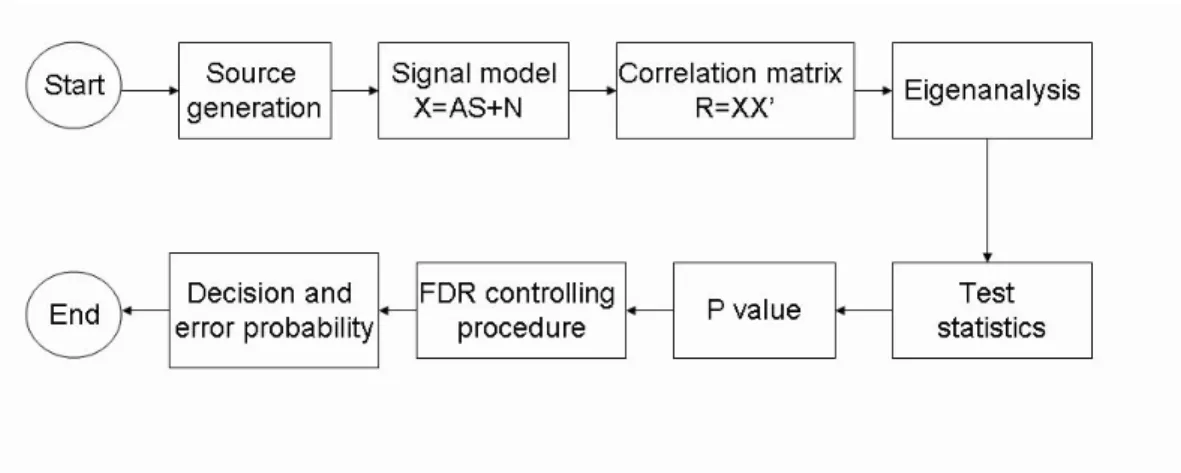
The whole simulation procedure is demonstrated as Fig. 4.2. First of all, we generate what kind of scenario we need to distinguish the advantages we have. Can it be outperform under closely located sources , few number of sensors, or weak sources situations? The source generation step decides what kind of scenario we try to test. Then, we collect data, use eigenanalysis to get sampled eigenvalues. Take these eigenvalues into the test statistics, depending on different proposed formulas we have discussed in chapter 2. After we adopt the test statistics, use the asymptotically chi-square distribution to get p value. Appendix will give some concept of how to get p value and why it is used in statistics area. Finally we

2 3 4 5 6 7 8 9 Number of sensors

sorted p value critical value

Figure 4.1: From the algorithm, the hypotheses set are rejected by the maximum number of the set which meet the criterion of procedure; that is, from the figure, the number of signals is decided from the minimum value of sorted p values greater than the corresponding compared values.

adopt Benjamini-Hochberg procedure to control the error rate.

Consider different data collected from different scenarios. First, the data is collected from an array with 7 sensors with inter-element spacings of half a wavelength. Three sources are generated from different directions, θ1, θ2 and θ3, respectively. We perform 100

Monte-Carlo runs and detected the number of signals decided by different approaches. Considering 7 sensors with spatial distance d, direction of arrivals (DOA) are 10o_{, 50}o _{and 80}o _and

snapshots T = 50. The significance level α is 0.01. The SNR varies from −5 dB to 0 dB in 0.5 dB steps. The setting of arrival angles are general case, which means that all the sources are separate with sufficient distance. If we use other set of DOA (Degree Of Arrival), such as

Figure 4.2: Simulation flow diagram.

10o _{and 50}o_{, we still can get the same result only if the locations of sources are not too close.}

(Generally, closely located sources have inference on the clarity of collected data. In order to avoid this inference, we separate the sources with sufficient degree, such 10o _{or wider, in}

this work.)

Fig. 4.3 shows that when the SNR is under −2 dB, the performance of FDR controlling is better than sphericity test which is without controlling of global level of multiple test. In this figure, we add conventional approach, MDL (∅ line), for comparison to reinforce the advantage of this approach. When the probability goes to one, the slight difference between these curves can be seen as the result of the setting of significance level and random parameters in simulation. Significance level is the largest type I error probability we can accept. Once we set the level, we can control the error probability at least under the level. Smaller significance level comes with smaller power. Generally, it is suggest to set the level between 0.2 to 0.01 depends on trade off. Under the same SNR, the proposed procedure has higher correct probability (increase around 5% to 15%) than the classical one.

Since one benefit of sphericity test comes from the closed locations of sources, we collect data from 20o _{and 30}o _{with 10 sensors and other parameters remain unchanged. Figure}

−4.5 −4 −3.5 −3 −2.5 −2 −1.5 −1 −0.5 0 SNR(dB)

FWE MDL FDR

Figure 4.3: Three sources are generated from 10o_{, 50}o _{and 80}o _{direction of arrival,}

respec-tively. The array consists 7 sensors with snapshots T = 50. α = 0.01 and SNR = [−5:0.5:0] dB

4.4 shows the advantage by using the multiple hypotheses control procedure with sphericity test. The only difference between the two simulations in Fig. 4.4 is the number of sensors. The underside plot is simulated under 5 sensors and the upper is 10. Under few number of sensors, we can see that even under the situation of few number of sensors, its performance still maintains better. If one moves the locations more close, such as the 25o _{and 30}o_{, the}

difference between the two curves will be closer; however, if we maintain the same difference between degrees, such as 40o _{and 50}o _{(the difference remains 10}o_{), the gap between two}