分組式差分進化演算法及其應用於模糊系統最佳化設計

(1)

國

立

交

通

大

學

電控工程研究所

博

士

論

文

分組式差分進化演算法及其應用於模糊系統最佳化設計

Group-Based Differential Evolution Algorithm and Its Application to Fuzzy

System Optimization

研究生：韓明峰

指導教授：林進燈張志永

(2)

分組式差分進化演算法及其應用於模糊系統最佳化設計

Group-Based Differential Evolution Algorithm and Its

Application to Fuzzy System Optimization

研究生：韓明峰

Student：Ming-Feng Han

指導教授：林進燈博士

Advisor：Dr. Chin-Teng Lin

張志永博士 Dr.

Jyh-Yeong Chang

國立交通大學

電控工程研究所

博士論文

A Dissertation

Submitted to Institute of Electrical Control Engineering

College of Electrical Engineering

National Chiao Tung University

in partial Fulfillment of the Requirements

for the Degree of

Doctor of Philosophy

in

Electrical Control Engineering

Jan. 2013

Hsinchu, Taiwan, Republic of China

(3)

i

分組式差分進化演算法及其應用於模糊系

統最佳化設計

研究生：韓明峰

指導教授：林進燈博士

張志永博士

國立交通大學電控工程研究所博士班

摘要

本篇論文主要分為兩個部分，第一部分，我們提出分組式差分進化演算法解決函數最佳化問題。該進化演算法使用兩種不同類型的突變運算，可解決傳統演算法常遇到的停滯問題，進而達到良好的演化搜尋能力。在演化程序中，依照個體之適應值，所有個體被區分為優等組與劣等組。優等組進行區域性的突變運算，劣等組進行全域性的突變運算。再藉由交配和選擇運算以產生新的子代。我們也提出一個新的適應學習策略為了避免人為設定參數問題，該策略能自動的找到最佳設定參數。在模擬中，我們測試 13 個函數最佳化問題。本論文所提出的演算法皆呈現良好的搜尋效能。第二部分，我們將分組式差分進化演算法應用在函數聯結之模糊系統最佳化設計上。在架構學習中，使用凝聚分群演算法自動地給予模糊系統最適合的模糊規則數。在參數學習中，群體將被拆善成數個子群體且每個子群體各自進化，最後可獲得最佳化的函數聯結之模糊系統。我們將與其他方法比較，以證實所提出的網路架構及其相關演算法之有效性。

(4)

ii

Group-Based Differential Evolution

Algorithm and Its Application to Fuzzy

System Optimization

Student：Ming-Feng Han

Advisor：Dr. Chin-Teng Lin

Dr.

Jyh-Yeong Chang

Institute of Electrical Control Engineering

National Chiao-Tung University

ABSTRACT

This dissertation consists of two major parts. In the first part, we propose a group-based differential evolution (GDE) algorithm for numerical optimization problems. The proposed GDE algorithm employs two different mutation operations to solve the stagnation problem and achieve good performance. Initially, all individuals in population are grouped into an inferior group and a superior group based on their fitness value. The inferior group uses the global mutation model. The superior group employs the local mutation model. Subsequently, crossover and selection operations are employed for the next generation. An adaptive strategy is also proposed to automatically find good parameters in the GDE algorithm. To validate the performance of the GDE algorithm, 13 numerical benchmark functions are tested. The simulation results indicate that the approach is effective and efficient. In the second part, we apply the GDE algorithm to function-link fuzzy system (FLFS) optimization.

(5)

iii

For structure learning, an agglomerative clustering algorithm is proposed to find the optimal number of fuzzy rules. For parameter learning, we use symbiotic learning method and GDE algorithm. The population is separated as subpopulations. Each subpopulation performs GDE algorithm to search the optimal parameter. The FLFS model with GDE learning algorithm (FLFS-GDE) is applied in real world prediction problems. Results of this dissertation demonstrate the effectiveness of the proposed methods.

(6)

iv

Acknowledgement

本篇論文能夠順利完成，首先要感謝兩位指導教授 - 林進燈老師與張志永老師。在二位教授豐富的學識、殷勤的教導及嚴謹的督促下，使我學習到許多的寶貴知識及在面對事情中應有的處理態度、方法，並且在研究與投稿論文的過程中，二位教授有許多深入的見解及看法且對於斟酌字句、思慮周延，更是我該學習的目標。師恩好蕩，指導提攜，銘感於心。同時也要感謝陶金旺教授、林正堅教授、蘇木春教授、楊谷洋教授等，在電機資訊工程領域各執牛耳的論文口試委員，能於百忙之中蒞臨指導，給予最寶貴的意見，使得本論文內容上更加完善。在艱辛的求學路上，謝謝這一路伴隨的學長和學弟們。感謝仕宇學長、東霖學長、肇廷學長及君玲學姐，因為你們的提點，讓我在研究上體悟更深成的道理，也感謝 Bio-CI Group 的成員：洋印與時慧，因為你們的存在，讓博士四年半的生活更加多采多姿，也祝福你們在未來的博士班口試順利。特別要感謝我的父親、母親、大姐、二姐、三姐，在這段日子中不斷的給予支持及鼓勵，讓我能夠專心於研究的工作並完成博士學位。最後誠摯地以本論文研究成果獻給我的師長、父母、家人及所有的朋友們。韓明峰民國 102 年 1 月 21 日

(7)

v

List of Tables

Table 3.1: Experimental results (Function 1－Function 8) of GDE, DE/rand/bin, DE/best/bin and DE/target-to-best/bin for low dimensional problems

(D=30), averaged over 50 independent runs. ...22

Table 3.2: Experimental results (Function 9－Function 11) of GDE, DE/rand/bin, DE/best/bin and DE/target-to-best/bin for low dimensional problems (D=30), averaged over 50 independent runs. ...23

Table 3.3: Experimental results ( Function 1－Function 8)of GDE, DE/rand/bin, DE/best/bin and DE/target-to-best/bin for high dimensional problems (D=100), averaged over 50 independent runs. ...30

Table 3.4: Experimental results ( Function 9－Function 13)of GDE, DE/rand/bin, DE/best/bin and DE/target-to-best/bin for high dimensional problems (D=100), averaged over 50 independent runs. ...31

Table 3.5: The rank table based on experimental results of GDE, DE/rand/bin, DE/best/bin and DE/target-to-best/bin for statistical comparison. ...38

Table 3.6: The result of Friedman test for statistical comparison. ...39

Table 3.7: Comparison with the proposed GDE algorithm and other methods (D=30), including RMEA,CEP, ALEP, BestLevy, NSDE and RTEP. ...40

Table 3.8: Comparison with the proposed GDE algorithm and advanced DE algorithms (D=30), including jDE, SaDE, ODE, SaCDE, DEGL and JADE ...41

Table 4.1: Initial parameters before training. ...61

Table 4.2: Performance of the GDE algorithm and the other algorithms for example 1. ...65

Table 4.3: The best performance of the FLFS-GDE model and other papers for example 1 ...66

Table 4.4: Performance of the GDE algorithm and the other algorithms for example 2. ...69

Table 4.5: The best performance of the FLFS-GDE model and other papers for example 2. ...70

Table 4.6: The performance of the GDE algorithm and other algorithms for example 3 ...76

Table 4.7: Comparison of the FLFS-GDE model and other papers for example 3. ...76

Table 4.8: Performance of the FLFS-GDE model and other algorithms for example 4 ...77

(9)

vii

List of Figures

Figure 2.1: The flow chart of the DE algorithm. Gen is the generation counter.. ...7 Figure 2.2: Illustration of the crossover process for NP=7 parameters.. ...10 Figure 3.1: The flow chart of the proposed GDE algorithm. GEN is the generation

counter... ...14 Figure 3.2: A concept of the self-adaptive parameter tuning strategy.... ...16 Figure 3.3: The best learning curve of GDE, DE/rand/bin, DE/best/bin and

DE/target-to-best/bin on 13 test function for low dimensional (D=30) problems. (a) Function 1: f1; (b) Function 2: f2; (c) Function 3: f3; (d)

Function 4: f4; (e) Function 5: f5; (f) Function 6: f6; (g) Function 7: f7; (h)

Function 8: f8; (i) Function 9: f9; (j) Function 10: f10; (k) Function 11: f11;

(l) Function 12: f12; (m) Function 13: f13. ...28

Figure 3.4: The best learning curve of GDE, DE/rand/bin, DE/best/bin and DE/target-to-best/bin on 13 test function for high dimensional (D=100) problems. (a) Function 1: f1; (b) Function 2: f2; (c) Function 3: f3; (d)

Function 4: f4; (e) Function 5: f5; (f) Function 6: f6; (g) Function 7: f7; (h)

Function 8: f8; (i) Function 9: f9; (j) Function 10: f10; (k) Function 11: f11;

(l) Function 12: f12; (m) Function 13: f13; ...36

Figure 4.1: The architecture of the functional-link fuzzy system. ...47 Figure 4.2: The overall learning process. ...48 Figure 4.3: A flow chart of the proposed agglomerative clustering algorithm for

discovering the optimal number of clusters. ...51 Figure 4.4: The result of proposed agglomerative clustering algorithm with respect to

different. ...52 Figure 4.5: The clustering results by the proposed algorithm with 4 (a) the result

of k =1, (b) the result of k =5, (c) the result of k =10, and (d) the result of

k =21. ...54

(10)

viii

Figure 4.7: A completed process of the subpopulation step.. ...57

Figure 4.8: A flow chart of the proposed GDE algorithm for the FLFS optimization.. ...59

Figure 4.9: The result of the agglomerative clustering algorithm for example 1. ...63

Figure 4.10: Training RMSEs of the DE, jDE, MODE and GDE algorithms at each performance evaluation for example 1. ...64

Figure 4.11: Prediction results of the FLFS-GDE model for example 1. Symbol "+" represents the desired results and "O" represents the actual results.. ...64

Figure 4.12: Prediction errors of the FLFS-GDE model for example 1.. ...65

Figure 4.13: The result of the agglomerative clustering algorithm for example 2.. ...68

Figure 4.14: Training RMSEs of the DE, jDE, MODE and GDE algorithms at each performance evaluation for example 2.. ...68

Figure 4.15: Symbol "+" represents the desired results and "O" represents the prediction results of the FLFS-GDE model for example 2.. ...69

Figure 4.17: Training RMSEs of the DE, jDE, MODE and GDE algorithms at each performance evaluation for example 3. ...72

Figure 4.18: The training output of the FLFS-GDE model for example 3. ...73

Figure 4.19: The testing output of the FLFS-GDE model for example 3.. ...73

Figure 4.20: The result of the agglomerative clustering algorithm for example 4. ...76

Figure 4.21: Prediction output of FPM-DEEMS model for example 4.. ...76

Figure 4.23: Symbol "+" represents desired and "O" represents prediction results of the FLFS-GDE model for example 5.. ...79

(11)

1

Chapter 1 Introduction

Evolutionary algorithms (EAs)[1-6] are population based stochastic optimization methods that are inspired by Darwin’s Theory of Evolution. EAs are able to deal with difficult objective functions which are, e.g., discontinuous, non-convex, multi-modal, non-linear and non-differentiable functions. Since engineering, economic and scientific problems include such difficult objectives, EAs have become popular optimization tools during the last couple of decades.

The optimization process of the EAs usually adopt stochastic search techniques that work with a set of individuals instead of a single individual, and use some evolution operators to naturally produce offsprings for the next generation. These algorithms include genetic algorithm (GA)[7-8], evolutionary programming (EP)[9-10], evolution strategies (ES)[11], particle swarm optimization (PSO)[12-13] and differential evolution (DE)[14-15] which are famous, effectual and classical search techniques.

The GA is a powerful optimization tool based on biological evolution mechanism and natural selection. This algorithm was first proposed and investigated by John Holland in 1973. The main idea of the GA follows the natural selection principle of selecting fittest individuals for the next generation and explores the relevant search space according to the evolutionary computing strategies. In the GA, chromosome is represented by a binary

(12)

2

bit-string. Generally, the initial population of GA is generated code “1” or“0” randomly for each design variable. Offsprings (new population) are produced by Reproduction. The Reproduction usually involves crossover and mutation. Crossover is the process of combining genetic building blocks from two or more parent vectors to form one or more new offspring. Mutation is the process of injecting random noise into offspring vectors to form a slightly different offspring individual, thereby increasing the genetic diversity of the population.

Evolution strategies (ES) were developed by Rechenberg and Schwefel[11]. This algorithm is an effective continuous function optimizer. In evolution process, ESs perform mutation operator as main operator to produce offspring. After mutating and evaluating all λ children, the (µ, λ)-ES selects the best µ children to become the next generation’s parents. Alternatively, the (µ + λ)-ES populates the next generation with the best µ vectors from the combined parent and child populations. The special case (µ + 1) is also referred to as steady-state ES.

A new population-based evolutionary algorithm, called particle swarm optimization (PSO), was proposed by Kennedy and Eberhart [12] in 1995. The population in PSO is referred to as a swarm. The PSO is based on simulations of social behaviors such as fish in a school, birds in a flock etc. A swarm in PSO consists of a number of particles. Each particle represents a potential solution of the optimization task. All of the particles iteratively discover a probable solution. Each particle moves to a new position according to the new velocity and the previous positions of the particle. The PSO has faster convergence than GA and ES to over a small number of generations.

In recent years, the DE algorithm is interested by researchers [14-35] among the EAs. The DE algorithm, proposed by Storn and Price [14-15] in 1998, is an efficient and effective global optimizer in the continuous search domain. It has been shown to perform better than the GA, ES and PSO over several numerical benchmarks [14-15, 19, 30, 34]. The DE

(13)

3

algorithm employs the difference of two randomly selected individuals as the source of random variations for the mutation operation. Subsequently, crossover and selection operations are used for generating offsprings. Many studies have applied the DE algorithm to difficult optimization problems and achieved better solutions[19, 28, 31]. However, the stagnation problem has been identified that the DE algorithm occasionally stops proceeding toward the global optimum [18-19]. The reason for stagnation problem is the limitation of the mutation operation model. In the DE algorithm, the mutation operation model always favors the exploration ability (DE/rand strategy) or the exploitation ability (DE/best strategy), which easily results in the blind search in individual space or the insufficient diversity in population. In order to deal with this problem, previous studies have proposed ideas to improve the mutation operation model. In [28, 31], the researchers have proposed a modiﬁed differential evolution (MODE) algorithm for an adaptive neural fuzzy network and locally recurrent neuro-fuzzy system optimazation. This MODE algorithm provides a convex type mutation model and cluster-based scheme to increase the diversity of the population. The concept of the tradeoff between the exploration ability and exploitation ability was proposed by Das et al.[18]. They designed a novel mutation model, called neighborhood-based mutation operation, to handle stagnation problem. In their paper, they utilized new mutation strategy and ring topology of neighborhood to find potential individuals in population. However, a single evolution model may not be suitable for various problems [21, 24, 27]. Therefore, other researchers which combine with other learning methods have proposed for solving the stagnation problem. Rahnamayan et al. [27] combined a opposition-based learning method and the DE algorithm, called opposition-based differential evolution (ODE). The ODE employs opposition-based optimization to choose the better solutions by simultaneously checking fitness of the opposite solution in the current population. The ODE possesses successfully increases diversity of the population. A combination of one-step k-Means clustering and multi-parent crossover operation in the DE algorithm was proposed

(14)

4

by Cai et al. [21]. Their method enhances the performance of the DE algorithm and balances the exploration ability and the exploitation ability in the evolutionary process. Noman and Iba [24] proposed an adaptive local search (ALS) algorithm to increase exploitation ability in the DE algorithm. The ALS algorithm uses a simple hill-climbing algorithm to adaptively determine the search length and effectively explore the neighborhood of each individual. Ali and Pant [36] applied a Cauchy mutation to improve the performance of the DE algorithm. The Cauchy mutation using Cauchy distribution randomly forces solutions to move to some other position. This method efficiently increases the probability of searching potential solutions in the DE algorithm. A combination of the fuzzy adaptive PSO algorithm and the DE algorithm, called FAPSO-DE model, was proposed by Niknam et al. [37]. They utilize two evolution processes to balance the exploration ability and exploitation ability for economic dispatch problems.

Unlike above mentioned studies, this dissertation proposes a new idea to solve the stagnation problem. This idea employs the inherent properties of the DE algorithm without depending on other learning algorithms. The idea combines two classical mutation strategies instead of a single mutation model. The two mutation strategies are composed of the DE/rand/bin operation and the DE/best/bin operation. The DE/rand/bin has powerful exploitation ability; and the DE/best/bin has efficient exploration ability. This dissertation uses the two operations to tradeoff between the exploration ability and the exploitation ability for solving the stagnation problem.

In this dissertation, a group-based differential evolution (GDE) algorithm is proposed for numerical optimization problems. The GDE algorithm provides a new process using the DE/rand/bin model and the DE/best/bin model in mutation operation. Initially, all individuals in population are grouped into an inferior group and a superior group based on their fitness value. The inferior group uses the DE/rand/bin mutation model for globally searching potential solutions and for maintaining the diversity of the population. The superior group

(15)

5

employs the DE/best/bin mutation model to efficiently search the neighborhood of the current best solution. Subsequently, crossover and selection operations are employed for the next generation. An adaptive strategy is also proposed in this dissertation. This strategy uses successful information to automatically tend to good parameters (factor F and crossover rate CR). It is thus helpful to enhance the robustness of the GDE algorithm. In order to validate the performance of the GDE algorithm, 13 well-known numerical benchmark functions with low dimensional problems and high dimensional problems are tested. Simulation results indicate that our approach is efficient. Comparison with other advance evolutionary algorithms, the proposed GDE algorithm performs better performance.

In addition, we also apply the proposed GDE algorithm to practical problems based on functional-link fuzzy systems (FLFS) optimization. Initially, the FLFS has no rules. The fuzzy rules are automatically generated by an agglomerative clustering algorithm. The agglomerative clustering algorithm (ACA) determines the optimal number of fuzzy rules for the FLFS. Subsequently, all free parameters are learned by the GDE algorithm for the FLFS optimization. During evolution process, the scale fact and crossover are adjusted by adaptive parameter tuning strategy. In the simulation, five prediction problems are tested to validate the performance of the proposed functional-link fuzzy system with the GDE algorithm (FLFS-GDE). The proposed FLFS-GDE model shows better prediction performance than other methods.

The overall objective of this dissertation is to develop a novel evolutionary algorithm and its related application. Organization and objectives of each chapter in this dissertation are as follows.

In Chapter 2, we introduce a basic DE algorithm and its evolution process. The DE algorithm employs the difference of two randomly selected individuals as the source of random variations for the mutation operation. Subsequently, crossover and selection operations are used for the next generation.

(16)

6

In Chapter 3, we present a new differential evolution algorithm, called group-based differential evolution algorithm for global optimization problems. This algorithm employs two mutation strategies instead of a single mutation model to tradeoff between the exploration ability and the exploitation ability for solving the stagnation problem. Furthermore, an adaptive strategy is also proposed to enhance the robustness of the GDE algorithm by an automatic process for finding good parameters. 13 well-known numerical benchmark functions are tested for simulations. The result shows significant differences between the proposed GDE algorithm and other methods.

In Chapter 4, the proposed GDE algorithm is applied to FLFS optimization for prediction problems. The learning process consists of rule generation phase and parameter learning phase. The rule generation phase can determine the optimal number of fuzzy rules using the agglomerative clustering algorithm. The parameter learning phase combines a subpopulation symbiotic evolution and a GDE algorithm. Initially, population is separated as many subpopulations according to the number of fuzzy rules. Each subpopulation performs the GDE algorithm for parameter learning. We also compare our method and other methods in simulations. Finally, conclusions and future works are summarized in Chapter 5.

(17)

7

Chapter 2 Differential Evolution

This section introduces a complete DE algorithm. The process of the DE algorithm, likes other EAs, produces offsprings for next generation by the mutation operation, the crossover operation and the selection operation. Figure 2.1 shows a standard flow chart of the DE algorithm. Initialize Population Performance Evaluation Mutation Operation Crossover Operation Selection Operation Meeting Termination Criterion ? Return Optimal Solution Gen=Gen+1 NO YES

(18)

8

Initially, a population of NP D-dimensional parameter vectors which represents the candidate solutions (individuals) is generated by uniformly random process. All individuals and search space are constrained by the prescribed minimum X_min(x_1,min,x_2,min,...,x_D_,min) and maximum X_max(x_1,max,x_2,max,...,x_D_,max) parameter bounds. A simple representation of i-th individual at the current generation Gen is shown as follows：

, ( ,1, , ,2, , ,3, ,..., , 1, , , , )

i Gen  xi Gen xi Gen xi Gen xi D Gen xi D Gen

X . (1) After Initial population production with NP individuals, fitness evaluation process measures quality of individuals to calculate the performance. The succeeding steps include the mutation operation, the crossover operation and the selection operation are explained in the following.

Mutation Operation

Each individual in the current generation is allowed to breed through mating with other randomly selected individuals from the population. This process randomly selected a parent pool of three individuals is formed to produce an offspring. Speciﬁcally, for each individual

, , 1, 2,...,

i gen i NP

X , where gen denotes the current generation, NP is population size, three random individuals,X_{r gen}_1, , X_r_2,_gen,X_r_3,_gen , X_r_4,_gen and X_r_5,_gen are selected from the population such that r1, r2, r3, r4 and r5 ∈ { 1, 2, . . . , NP } and i r1 r2r3r4r5. This way, a parent pool of four individuals is formed to produce an offspring. The following are different mutation strategies frequently used in the literature:

, 1, 2, 3,

DE/rand/bin: V_{i gen} X_{r gen}F(X_r _genX_r _gen) (2)

, , 2, 3,

(19)

9

, 1, , 1,

2, 3,

DE/target-to-best/bin: ( )

( )

i gen r gen gbest gen r gen

r gen r gen F F      V X X X X X (4) , 1, 2, 3, 4, 5, DE/rand/bin/2: ( ) ( )

i gen r gen r gen r gen

r gen r gen F F      V X X X X X (5) , , 2, 3, 4, 5, DE/best/bin/2: ( ) ( )

i gen gbest gen r gen r gen

r gen r gen F F      V X X X X X (6)

where Fis scaling factors[0,1], X_{gbest gen}_, is the best-so-far individual (i.e., X_{gbest gen}_,

keeps best ﬁtness value up to now in the population). For various problems, the DE algorithm usually employs different mutation strategy. The DE/rand/bin/ mutation and DE/rand/bin/2 mutation which have more exploration ability are suitable for multimodal problems. The “DE/best/bin”, “DE/best/bin/2” “DE/target-to-best” mutations which consider the current best information in generation are more suitable for unimodal problems.

Crossover Operation

After the mutation operation, The DE algorithm uses a crossover operation, often referred to as discrete recombination, in which the mutated individual V_{i gen}_, is mated with

,

i gen

X and generates the offspringU_{i gen}_, . The elements of an individualU_{i gen}_, are inherited from X_{i gen}_, and V_{i gen}_, , which are determined by a parameter called crossover probability (CR ∈ [0, 1]), as follows: , , , , , , , if rand( ) CR , if rand( ) > CR i d gen i d gen i d gen d d      V U X (5)

(20)

10

individual vector, r (d) ∈ [0, 1] is the dth evaluation of a random number generator. Figure 2.2 gives an example of the crossover mechanism for 7-dimensional vectors.

D=1 2 3 4 5 6 7

Xi,Gen Vi,Gen U,Gen

D=1 2 3 4 5 6 7 D=1 2 3 4 5 6 7 Target vector Mutant vector Trial vector r(3)<=CR r(4)<=CR r(6)<=CR

Figure 2.1 : Illustration of the crossover process for NP=7 parameters.

Selection Operation

The DE algorithm applies selection operation to determine whether the individual survives to the next generation. A knockout competition is played between each individual

,

i gen

X and its offspringU_{i gen}_, , and the winner is selected deterministically based on objective function values and is then promoted to the next generation. The selection operation is described as , , , , 1 , , if fitness( ) < fitness( ) , otherwise

i gen i gen i gen

i gen i gen     X X U X U (6)

wherefitness( )z is the fitness value of individual z. After the selection operation, the population obtains better ﬁtness value or remains the same ﬁtness value, but never deteriorates.

(21)

11

Chapter 3 Group-Based Differential Evolution

3.1 A GDE Algorithm

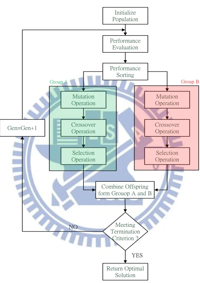
In the DE algorithm, mutation operation which leads a successful evolution performance is a principal operator. For various problems, we often employ different mutation strategy in the DE algorithm. However, choosing suitable mutation strategy which deals with a practical problem is difficult. Therefore, we propose the GDE algorithm with the exploration ability and the exploitation ability, which combines two mutation strategies to solve practical problems. A flow chart of the GDE algorithm is shown in Figure 3.1.

In first step of the GDE algorithm, a population of NP D-dimensional individuals is generated by uniformly random process, and evaluated for the fitness value of all individuals. A sorting process arranges all individuals based on their fitness value as

1 2 ... NP 1 NP

fitness  fitness   fitness   fitness _for _minimum _objective _problems.

According to fitness value, all individuals are partitioned into an inferior group and a superior group, called the Group A and the Group B. The Group A, including NP/2 worse individuals, performs global search to increase the diversity of the population and widely find potential solutions. Other NP/2 individuals for the Group B perform local search to actively detect better solutions nearby current best solution. A complete mutation operation is shown for the Group A and the Group B as follows.

(22)

12 , , 1 , 2 , G r o u p A : V_{i g e n} X _{i g e n}F X_a ( _r_{g e n}X _r )_{g e n} (7) , , 3 , 4 , G r o u p B : V_{i g e n} X _{g b e s t g e n}F X (_b _rX_{g e n} _r) _{g e n} (8) Where Fa and Fb are scale factors,X_{r gen}_1, ,X_r_2,_gen, X_r_3,_gen and X_r_4,_gen are random selected

from the population, andir1r2r3r4,the X_{gbest gen}_, is the best-so-far individual in the population.

After mutation operation, The GDE algorithm uses a crossover operation, often referred to as discrete recombination, in which the mutated individual V_{i gen}_, is mated withX_{i gen}_, and generates the offspringU_{i gen}_, . Equation 9 presents the crossover operation for the Group A and the Group B. If the random number rand(d) is smaller than the CR value, the variable of the mutated individual V_{i d gen}_{, ,} is chosen to the variable of the trial vector U_{i d gen}_{, ,} . Otherwise, the variable of the target vector X_{i d gen}_{, ,} is selected to the variable of the trial vector U_{i d gen}_{, ,}

. , , , , , , , if rand( ) CR , if rand( ) > CR i d gen i d gen i d gen d d      V U X (9)

where d = 1, 2, . . . , D denotes the dth element of individual vectors, D is total element of individual vector, CR ∈ [0, 1],rand(d) ∈ [0, 1] is the dth evaluation of a random number generator. The mutation and crossover operators are used to diversify the search space in terms of the optimization problems.

Selection operation is used to determine whether the individual survives to the next generation. A knockout competition is played between each individual X_{i gen}_, and its offspringU_{i gen}_, , and the winner is selected deterministically based on objective function values and is then promoted to the next phase. After the selection operation, the population gets better or remains the same in ﬁtness value, but never deteriorates.

(23)

13

The conventional DE only utilizes DE/best or DE/rand mutation to deal with problems. The proposed GDE algorithm employed two mutation operations to maintain useful diversity in the population and increase the search capability. It is worth noting that DE/best/bin and DE/rand/bin are a special case in the proposed GDE algorithm when population = Group A and population = Group B. Thereby, the proposed GDE algorithm has more variety than conventional DE algorithm for various problems. In this dissertation, we set the size of the Group A= Group B=NP/2 because it obtained the best performance in the present study.

(24)

14 Initialize Population Performance Evaluation Meeting Termination Criterion ? Return Optimal Solution Gen=Gen+1 NO YES Performance Sorting Mutation Operation Crossover Operation Selection Operation Mutation Operation Crossover Operation Selection Operation Combine Offspring form Grouop A and B

Group A Group B

(25)

15

3.2 A Self-Adaptive Parameter Tuning Strategy

Parameter control which can directly influence the convergence speed and search capability is an important task in the EAs [12, 19]. However, conventional DE algorithm always used trial-and-error method for choosing suitable parameter requires multiple optimization runs. Based on this consideration, different adaptive or self-adaptive mechanisms [16, 18, 22, 25, 32] have been recently introduced to dynamically update the control parameters without a user’s prior knowledge of the relationship between the parameter setting and the characteristics of optimization problems. In this section, we propose a generalized self-adaptive approach to control parameter the F and the CR for the Group A (inferior) and the Group B (superior). The concept of the proposed parameter tuning strategy is shown in Figure 3.2. The generalized scheme is designed as follows：

(1) Assume new parameters G_i[G_min,G_max] , 1 i NP. The G_i is composed of and

i i

F CR for individualx . We set a initial center _i G_center

(2) Set g  g 1 and randomly generate G by Gaussian distribution (_i G_center, 0.2 ) for every individualx . _i

(3) After evolution process, the G that is able to make the offspring _i xi g, 1 of x to i

successfully enter the next generation. That is, a good parameter value G will be _i

marked and recorded in our algorithm. The successful parameter value G_success( )k and

ﬁtness improvements( ), where =1,2,...,k k N_g_₁

sucess( ) [ sucess, k, sucess, k]

G k  F CR (10)





2 , 1 ( )k fitness x( _{k g} ) fitness x( _k)   _  (11)

(26)

16 (4) Update the parameter center according to

, 1

(1 )

center center center g

G  w G  w G _ (12) where the weight w is determined by

1 1 g g g N w N N     (13)

and G_{center g}_, _₁ is the weighted mean of values in G_sucess:

, 1 sucess 1 1 ( ) ( ) ( ) g g N center g N k k k G G k k      







(14)

(5) If N_g_₁N_g, then update theN_g_₁ as follows

1 0.9

g g

N _  N (15) (6) Go to Step 2 for the next generation until a stopping criterion is satisﬁed.

Individual 1 Individual 2 . . . Individual NP F1 CR1 F2 CR2 FNP CRNP . . . . . . G1 G2 GNP success( ), ( ) G k



k center

G

Gaussian Distribution Collection Updating Assignment

(27)

17

3.3 Simulation

In order to verify the performance of proposed algorithm, a set of thirteen classical benchmark test functions [38-39] is used in this simulation. The analytical form of these functions is given in section 3.3.1. The GDE algorithm is compared with three classic DE algorithms, including the DE/rand/bin, the DE/best/bin and the DE/target-to-best/bin algorithms. In all simulations, we set the parameters of the GDE algorithm to be fixed, initial

Fa= 0.5, initial Fb =0.8, initial CRa=0.9 ,initial CRb =0.9. The parameter setting for three

classic DE algorithms is recommended by other papers as follows. For DE/rand/bin model, the F=0.5 and the CR=0.9 [15, 22, 32]；For DE/bes/bin model, the F=0.8 and the CR=0.9 [18]；For DE/target-to-best/bin, the F=0.8 and the CR=0.9[20].

Many papers have used the same parameter setting to solve their problems. In this simulation, we set the population size NP to be 100 and 400 in the case of D = 30, and D = 100, respectively. All results reported in this section are obtained based on 50 independent runs. In addition, Section 3.3.3 demonstrates significant difference results based on statistical comparison process. A complete comparison with other evolutionary algorithms, such as RMEA[45],CEP[30], ALEP[43], BestLevy[43], NSDE[40], RTEP[44], jDE[33,47], SaDE[26], ODE[27], SaCDE[16], DEGL[18] and JADE[22,46], is presented in Section 3.3.4.

(28)

18

3.3.1 Test Functions

In this section, we introduce thirteen numerical functions for verifying the performance of proposed GDE algorithm. Based on their properties, the functions can be divided into two problems as unimodal function problem and multimodal function problem. f1– f4 are

continuous unimodal functions. f5 is a discontinuous step function, and f6 is a noisy quartic

function. f7 is the Rosenbrock function which is multimodal function problem for D > 3 [39].

f8– f13 are multimodal and the number of their local minima increases exponentially with the

problem dimension [40]. In addition, f8 is the only bound-constrained function investigated

in this paper. All these functions have an optimal value at zero. Completed functions are described as follows:

(1) Function 1 ：Sphere function

2 1 1

( )

-100

100

D i i i

f

x





　，

 

(2) Function 2 ：Schwefel’s problem_a

2 1 1

-10

10

D D i i i i i

f

x

 









　 ,

 

(3) Function 3 ：Schwefel’s problem_b

2 3 1 1

-100

100

D i i i i j

f

x

 







_

_

 





 

　 ,

(4) Function 4 ：Schwefel’s problem_c

4

max

i

-100

i

100

i

(29)

19

(5) Function 5 ：Schwefel’s problem_d





2 5 1

0.5 -100

100

D i i i

f

x







,

 

(6) Function 6 ：Schwefel’s problem_e





4 6 1

0,1

-1.28

1.28

D i i i

f

ix

rand

x







,

 

(7) Function 7 ：Rosenbrock’s function

2 2 7 1 1

100(

) (

1)

-30

30

D i i i i i

f

x

_

x











_







_

,

 

(8) Function 8 ：Schwefel’s function

8 1

sin

418.98288727243369

-500

500

D i i i i

f

x

D

x







 

,

 

(9) Function 9 ：Rastrigin’s function





9 1

10 cos(2

) 10

-5.12

5.12

D i i i i

f

x



x









,

 

(10) Function 10 ：Ackley’s function

2 10

1 1

1

1 20 exp

0.2 exp

cos(2

)

20 -32

32

D D i i i i i

f

x

e

D

x



 





_

_

 



_





_



_

_











 



,

(30)

20

(11) Function 11 ：Griewank’s function

2 11 1 1

1 cos(

) 1

-600

600 4000

D D i i i i i

x

f

x

i

 











,

 

(12) Function 12 ：Generalized penalized function_1

1 2 2 2 2 12 1 1 1 1

10 sin (

)

(

1) 1 10 sin (

)

(

1)

( ,10,100, 4)

where

1

1 (

1),

4 (

) , if

( , , , )

(

) , if

0 , otherwise

D i i D i D i i i i m i i m i i i

f

y

D

u x

y

x

k x

a

x

a

u x a k m

k

x

a

x

a



_



_

  



_

_





_





_



_





_







 











 

 



-50

x

_i

50 







 

(13) Function 13 ：Generalized penalized function_2

1 2 2 2 2 2 13 1 1 1 1

1 sin (3

)

(

1) 1 sin (3

)

(

1) 1 sin (2

)

10 ( ,10,100, 4)

where

(

) , if

( , , , )

(

) , if

0 , otherwise

D i i D D i D i i m i i m i i i

f

x

u x

k x

a

x

a

u x a k m

k

x

a

x

a







_



 



_

_

_

_





_





_



_





_



_

_













 

 



-50

x

_i

50 









 

(31)

21

3.3.2 Low-Dimensional Problems

In this simulation, the GDE, DE/rand/bin, DE/best/bin and DE/target-to-best/bin algorithms are applied to low dimensional problems on 13 benchmark test functions. Table 3.1 and Table 3.2 show the detailed performance of the GDE, DE/rand/bin, DE/best/bin and DE/target-to-best/bin algorithms, including the mean, best and worst performance over 50 independent runs. This table indicates that the GDE algorithm obviously achieves better performance than the DE/rand/bin, DE/best/bin and DE/target-to-best/bin algorithms on 13 benchmark test functions. Especially, the GDE algorithm searches the global optimal solution at zero on the Function 5 and the Function 11. Focus on three classical DE algorithms, the DE/target-to-best/bin algorithm often obtains a better performance than the DE/rand/bin and DE/best/bin algorithms on 13 benchmark test functions. The DE/rand/bin obtains obvious difference on the Function 11 and the Function 13 among three classical DE algorithms.

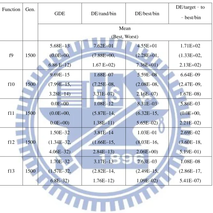
The learning curve of the GDE, DE/rand/bin, DE/best/bin and DE/target-to-best/bin algorithms on 13 test function for low dimensional (D=30) problems is shown in Figure 3.3. This Figure presented that the GDE algorithm possesses speedier convergence than the DE/rand/bin, DE/best/bin and DE/target-to-best/bin algorithms on 13 benchmark test functions. An interesting case is shown in Figure 3(h) and Figure 3(i). The DE/rand/bin, DE/best/bin and DE/target-to-best/bin algorithms are stopped at locally optimal solutions on the Function 9and the Function 10. The GDE algorithm maintains a continued convergence to find the optimal solutions. It is shown that the proposed GDE algorithm successfully overcomes the stagnation problem for low dimensional problems.

(32)

22

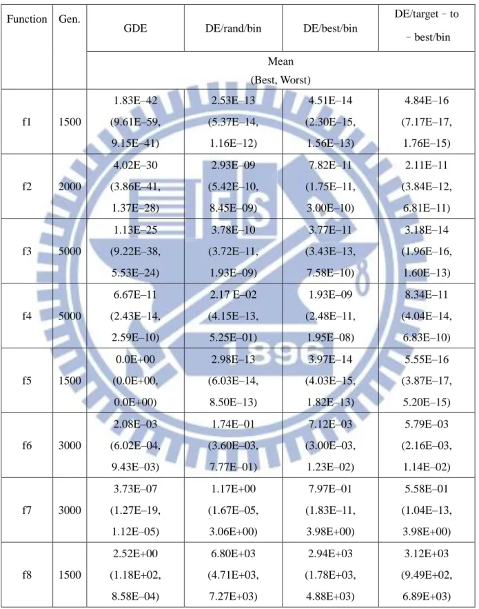
Table 3.1: Experimental results (Function 1－Function 8)of GDE, DE/rand/bin, DE/best/bin and DE/target-to-best/bin for low dimensional problems (D=30), averaged over 50 independent runs.

Function Gen.

GDE DE/rand/bin DE/best/bin

DE/target–to –best/bin Mean (Best, Worst) f1 1500 1.83E–42 (9.61E–59, 9.15E–41) 2.53E–13 (5.37E–14, 1.16E–12) 4.51E–14 (2.30E–15, 1.56E–13) 4.84E–16 (7.17E–17, 1.76E–15) f2 2000 4.02E–30 (3.86E–41, 1.37E–28) 2.93E–09 (5.42E–10, 8.45E–09) 7.82E–11 (1.75E–11, 3.00E–10) 2.11E–11 (3.84E–12, 6.81E–11) f3 5000 1.13E–25 (9.22E–38, 5.53E–24) 3.78E–10 (3.72E–11, 1.93E–09) 3.77E–11 (3.43E–13, 7.58E–10) 3.18E–14 (1.96E–16, 1.60E–13) f4 5000 6.67E–11 (2.43E–14, 2.59E–10) 2.17 E–02 (4.15E–13, 5.25E–01) 1.93E–09 (2.48E–11, 1.95E–08) 8.34E–11 (4.04E–14, 6.83E–10) f5 1500 0.0E+00 (0.0E+00, 0.0E+00) 2.98E–13 (6.03E–14, 8.50E–13) 3.97E–14 (4.03E–15, 1.82E–13) 5.55E–16 (3.87E–17, 5.20E–15) f6 3000 2.08E–03 (6.02E–04, 9.43E–03) 1.74E–01 (3.60E–03, 7.77E–01) 7.12E–03 (3.00E–03, 1.23E–02) 5.79E–03 (2.16E–03, 1.14E–02) f7 3000 3.73E–07 (1.27E–19, 1.12E–05) 1.17E+00 (1.67E–05, 3.06E+00) 7.97E–01 (1.83E–11, 3.98E+00) 5.58E–01 (1.04E–13, 3.98E+00) f8 1500 2.52E+00 (1.18E+02, 8.58E–04) 6.80E+03 (4.71E+03, 7.27E+03) 2.94E+03 (1.78E+03, 4.88E+03) 3.12E+03 (9.49E+02, 6.89E+03)

(33)

23

Table 3.2: Experimental results (Function 9 － Function 13)of GDE, DE/rand/bin, DE/best/bin and DE/target-to-best/bin for low dimensional problems (D=30), averaged over 50 independent runs.

Function Gen.

DE/target–to –best/bin Mean (Best, Worst) f9 1500 5.68E–13 (0.0E+00, 6.86 E–12) 7.62E+01 (7.88E+00, 1.67 E+02) 4.55E+01 (2.28E+01, 7.36E+01) 1.71E+02 (1.33E+02, 2.13E+02) f10 1500 9.69E–15 (7.99E–15, 3.28E–14) 1.68E–07 (7.25E–08, 3.31E–07) 5.59E–08 (2.08E–08, 2.16E–07) 6.64E–09 (2.47E–09, 1.67E–08) f11 1500 0.0E+00 (0.0E+00, 0.0E+00) 1.08E–12 (5.87E–14, 1.38E–11) 8.31E–03 (6.32E–15, 5.65E–02) 5.86E–03 (0.0E+00, 2.21E–02) f12 1500 1.50E–32 (1.34E–32, 4.06E–32) 3.81E–14 (1.66E–15, 2.84E–13) 1.03E–01 (8.03E–16, 2.06E+00) 2.69E–02 (3.60E–18, 5.19E–01) f13 1500 1.70E–32 (1.57E–32, 6.8E–32) 3.17E–13 (2.82E–14, 1.76E–12) 2.63E–03 (2.49E–15, 1.09E–02) 1.08E–08 (2.86E–17, 5.41E–07)

(34)

24 (a) (b) (c) 0 500 1000 1500 10-60 10-40 10-20 100 1020 Generation Lo g of F itn es s V au le DE/rand/bin DE/best/bin DE/target-to-best/bin GDE 0 500 1000 1500 2000 10-60 10-40 10-20 100 1020 Generation Lo g of F itn es s V au le DE/rand/bin DE/best/bin DE/target-to-best/bin GDE 0 1000 2000 3000 4000 5000 10-40 10-30 10-20 10-10 100 1010 Generation Lo g of F itn es s V au le DE/rand/bin DE/best/bin DE/target-to-best/bin GDE

(35)

25 (d) (e) (f) 0 1000 2000 3000 4000 5000 10-15 10-10 10-5 100 105 Generation Lo g of F itn es s V au le DE/rand/bin DE/best/bin DE/target-to-best/bin GDE 0 500 1000 1500 10-40 10-30 10-20 10-10 100 1010 Generation Lo g of F itn es s V au le DE/rand/bin DE/best/bin DE/target-to-best/bin GDE 0 500 1000 1500 2000 2500 3000 10-4 10-2 100 102 104 Generation Lo g of F itn es s V au le DE/rand/bin DE/best/bin DE/target-to-best/bin GDE

(36)

26 (g) (h) (i) 0 500 1000 1500 2000 2500 3000 10-20 10-10 100 1010 Generation Lo g of F itn es s V au le DE/rand/bin DE/best/bin DE/target-to-best/bin GDE 0 500 1000 1500 10-4 10-2 100 102 104 106 Generation Lo g of F itn es s V au le DE/rand/bin DE/best/bin DE/target-to-best/bin GDE 0 500 1000 1500 10-15 10-10 10-5 100 105 Generation Lo g of F itn es s V au le DE/rand/bin DE/best/bin DE/target-to-best/bin GDE

(37)

27 (j) (k) (l) 0 500 1000 1500 10-15 10-10 10-5 100 105 Generation Lo g of F itn es s V au le DE/rand/bin DE/best/bin DE/target-to-best/bin GDE 0 500 1000 1500 10-20 10-15 10-10 10-5 100 105 Generation Lo g of F itn es s V au le DE/rand/bin DE/best/bin DE/target-to-best/bin GDE 0 500 1000 1500 10-40 10-30 10-20 10-10 100 1010 Generation Lo g of F itn es s V au le DE/rand/bin DE/best/bin DE/target-to-best/bin GDE

(38)

28 (m)

Figure 3.3. The best learning curve of GDE, DE/rand/bin, DE/best/bin and DE/target-to-best/bin on 13 test function for low dimensional (D=30) problems. (a) Function 1: f1; (b) Function 2: f2; (c) Function 3: f3; (d) Function 4: f4; (e) Function 5: f5; (f) Function

6: f6; (g) Function 7: f7; (h) Function 8: f8; (i) Function 9: f9; (j) Function 10: f10; (k)

Function 11: f11; (l) Function 12: f12; (m) Function 13: f13.

0 500 1000 1500 10-40 10-30 10-20 10-10 100 1010 Generation Lo g of F itn es s V au le DE/rand/bin DE/best/bin DE/target-to-best/bin GDE

(39)

29

3.3.3 High-Dimensional Problems

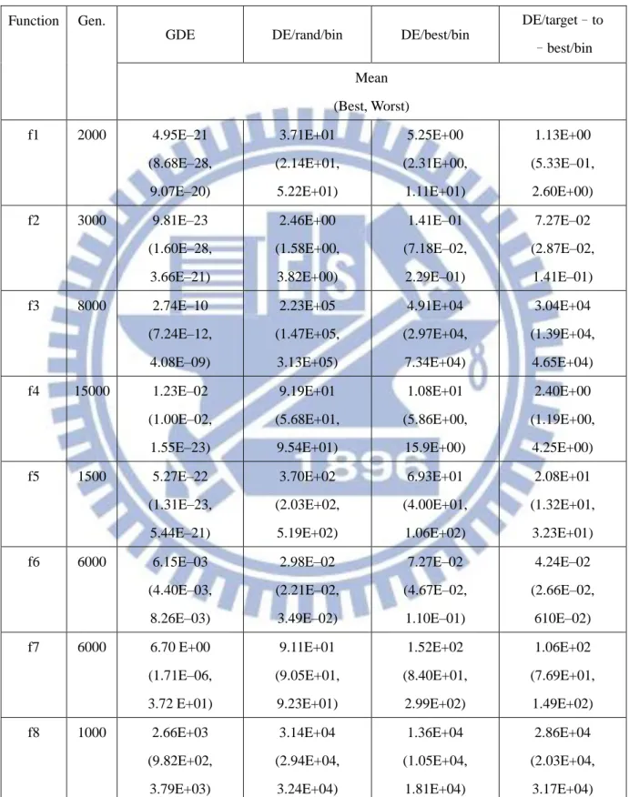
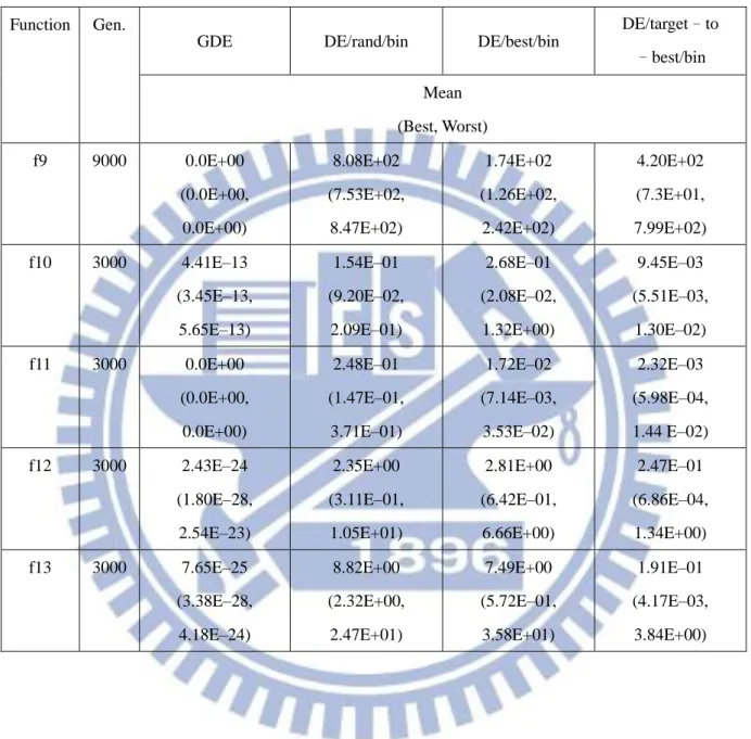
In order to verify the capability of algorithm on high dimensional problems, the GDE, DE/rand/bin, DE/best/bin and DE/target-to-best/bin algorithms are applied to 13 benchmark test functions. Table 3.3 and Table 3.4 show the detailed performance of the GDE, DE/rand/bin, DE/best/bin and DE/target-to-best/bin algorithms, including the mean, best and worst performance over 50 independent runs. Obviously, all algorithms are difficult to find optimal solutions caused by high dimensional problem. In Tables, the GDE algorithm obtains better performance than the DE/rand/bin, DE/best/bin and DE/target-to-best/bin algorithms on 13 benchmark test functions. Notice that the GDE algorithm efficiently searches a global optimal solution at zero on the Function 9 and the Function 11. Among three classical DE algorithms, the DE/target-to-best/bin algorithm obtains obvious difference on the Function 9 and the Function 11.

The learning curve of the GDE, DE/rand/bin, DE/best/bin and DE/target-to-best/bin algorithms on 13 test function for high dimensional (D=100) problems is shown in Figure 3.4. In this Figure, the GDE algorithm also presents speedier convergent curves than other algorithms on high dimensional functions. The stagnation situation is also happened when the DE/rand/bin, DE/best/bin and DE/target-to-best/bin algorithms are performed in Figure 3(b), Figure 3(c), Figure 3(e), Figure 3(g) and Figure 3(i). The GDE algorithm continuously maintains a convergent curve on the Function 2, Function 3, Function 5, Function 7 and Function 9. In this paper, the simulation result show that the proposed GDE algorithm obviously achieves better performance and successfully overcomes the stagnation situation for low dimensional problems and low dimensional problems.

(40)

30

Table 3.3: Experimental results ( Function 1 － Function 8) of GDE, DE/rand/bin, DE/best/bin and DE/target-to-best/bin for high dimensional problems (D=100), averaged over 50 independent runs.

Function Gen.

DE/target–to –best/bin Mean (Best, Worst) f1 2000 4.95E–21 (8.68E–28, 9.07E–20) 3.71E+01 (2.14E+01, 5.22E+01) 5.25E+00 (2.31E+00, 1.11E+01) 1.13E+00 (5.33E–01, 2.60E+00) f2 3000 9.81E–23 (1.60E–28, 3.66E–21) 2.46E+00 (1.58E+00, 3.82E+00) 1.41E–01 (7.18E–02, 2.29E–01) 7.27E–02 (2.87E–02, 1.41E–01) f3 8000 2.74E–10 (7.24E–12, 4.08E–09) 2.23E+05 (1.47E+05, 3.13E+05) 4.91E+04 (2.97E+04, 7.34E+04) 3.04E+04 (1.39E+04, 4.65E+04) f4 15000 1.23E–02 (1.00E–02, 1.55E–23) 9.19E+01 (5.68E+01, 9.54E+01) 1.08E+01 (5.86E+00, 15.9E+00) 2.40E+00 (1.19E+00, 4.25E+00) f5 1500 5.27E–22 (1.31E–23, 5.44E–21) 3.70E+02 (2.03E+02, 5.19E+02) 6.93E+01 (4.00E+01, 1.06E+02) 2.08E+01 (1.32E+01, 3.23E+01) f6 6000 6.15E–03 (4.40E–03, 8.26E–03) 2.98E–02 (2.21E–02, 3.49E–02) 7.27E–02 (4.67E–02, 1.10E–01) 4.24E–02 (2.66E–02, 610E–02) f7 6000 6.70 E+00 (1.71E–06, 3.72 E+01) 9.11E+01 (9.05E+01, 9.23E+01) 1.52E+02 (8.40E+01, 2.99E+02) 1.06E+02 (7.69E+01, 1.49E+02) f8 1000 2.66E+03 (9.82E+02, 3.79E+03) 3.14E+04 (2.94E+04, 3.24E+04) 1.36E+04 (1.05E+04, 1.81E+04) 2.86E+04 (2.03E+04, 3.17E+04)

(41)

31

Table 3.4: Experimental results ( Function 9 － Function 13) of GDE, DE/rand/bin, DE/best/bin and DE/target-to-best/bin for high dimensional problems (D=100), averaged over 50 independent runs.

Function Gen.

DE/target–to –best/bin Mean (Best, Worst) f9 9000 0.0E+00 (0.0E+00, 0.0E+00) 8.08E+02 (7.53E+02, 8.47E+02) 1.74E+02 (1.26E+02, 2.42E+02) 4.20E+02 (7.3E+01, 7.99E+02) f10 3000 4.41E–13 (3.45E–13, 5.65E–13) 1.54E–01 (9.20E–02, 2.09E–01) 2.68E–01 (2.08E–02, 1.32E+00) 9.45E–03 (5.51E–03, 1.30E–02) f11 3000 0.0E+00 (0.0E+00, 0.0E+00) 2.48E–01 (1.47E–01, 3.71E–01) 1.72E–02 (7.14E–03, 3.53E–02) 2.32E–03 (5.98E–04, 1.44 E–02) f12 3000 2.43E–24 (1.80E–28, 2.54E–23) 2.35E+00 (3.11E–01, 1.05E+01) 2.81E+00 (6.42E–01, 6.66E+00) 2.47E–01 (6.86E–04, 1.34E+00) f13 3000 7.65E–25 (3.38E–28, 4.18E–24) 8.82E+00 (2.32E+00, 2.47E+01) 7.49E+00 (5.72E–01, 3.58E+01) 1.91E–01 (4.17E–03, 3.84E+00)

(42)

32 (a) (b) (c) 0 500 1000 1500 2000 10-30 10-20 10-10 100 1010 Generation Lo g of F itn es s V au le DE/rand/bin DE/best/bin DE/target-to-best/bin GDE 0 500 1000 1500 2000 2500 3000 10-40 10-20 100 1020 1040 1060 Generation Lo g of F itn es s V au le DE/rand/bin DE/best/bin DE/target-to-best/bin GDE 0 2000 4000 6000 8000 10-15 10-10 10-5 100 105 1010 Generation Lo g of F itn es s V au le DE/rand/bin DE/best/bin DE/target-to-best/bin GDE

(43)

33 (d) (e) (f) 0 5000 10000 15000 10-2 10-1 100 101 102 Generation Lo g of F itn es s V au le DE/rand/bin DE/best/bin DE/target-to-best/bin GDE 0 500 1000 1500 10-30 10-20 10-10 100 1010 Generation Lo g of F itn es s V au le DE/rand/bin DE/best/bin DE/target-to-best/bin GDE 0 1000 2000 3000 4000 5000 6000 10-4 10-2 100 102 104 Generation Lo g of F itn es s V au le DE/rand/bin DE/best/bin DE/target-to-best/bin GDE

(44)

34 (g) (h) (i) 0 1000 2000 3000 4000 5000 6000 10-10 10-5 100 105 1010 Generation Lo g of F itn es s V au le DE/rand/bin DE/best/bin DE/target-to-best/bin GDE 0 200 400 600 800 1000 102 103 104 105 Generation Lo g of F itn es s V au le DE/rand/bin DE/best/bin DE/target-to-best/bin GDE 0 2000 4000 6000 8000 10-15 10-10 10-5 100 105 Generation Lo g of F itn es s V au le DE/rand/bin DE/best/bin DE/target-to-best/bin GDE

(45)

35 (j) (k) (l) 0 500 1000 1500 2000 2500 3000 10-15 10-10 10-5 100 105 Generation Lo g of F itn es s V au le DE/rand/bin DE/best/bin DE/target-to-best/bin GDE 0 500 1000 1500 2000 2500 3000 10-20 10-15 10-10 10-5 100 105 Generation Lo g of F itn es s V au le DE/rand/bin DE/best/bin DE/target-to-best/bin GDE 0 500 1000 1500 2000 2500 3000 10-30 10-20 10-10 100 1010 Generation Lo g of F itn es s V au le DE/rand/bin DE/best/bin DE/target-to-best/bin GDE

(46)

36 (m)

Figure 3.4 : The best learning curve of GDE, DE/rand/bin, DE/best/bin and DE/target-to-best/bin on 13 test function for high dimensional (D=100) problems. (a) Function 1: f1; (b) Function 2: f2; (c) Function 3: f3; (d) Function 4: f4; (e) Function 5: f5; (f)

Function 6: f6; (g) Function 7: f7; (h) Function 8: f8; (i) Function 9: f9; (j) Function 10: f10; (k)

Function 11: f11; (l) Function 12: f12; (m) Function 13: f13;

0 500 1000 1500 2000 2500 3000 10-30 10-20 10-10 100 1010 Generation Lo g of F itn es s V au le DE/rand/bin DE/best/bin DE/target-to-best/bin GDE

(47)

37

3.3.4 Statistical Comparison Using Friedman test

In order to understand the significant difference between the GDE and other algorithms over multiple test functions, this paper performed a statistical procedure based on the Friedman test [41, 42] with the corresponding post-hoc tests. We set the GDE algorithm as the control algorithm to compare with other algorithms. The performance of algorithm is significant difference if the corresponding average ranks differ by at least the critical difference (CD) 0.05 ( 1) 6 j j CD q T   , (16) where j is the number of algorithms, T is the number of test functions, and critical values

0.05

q =2.569 can be found in [42].

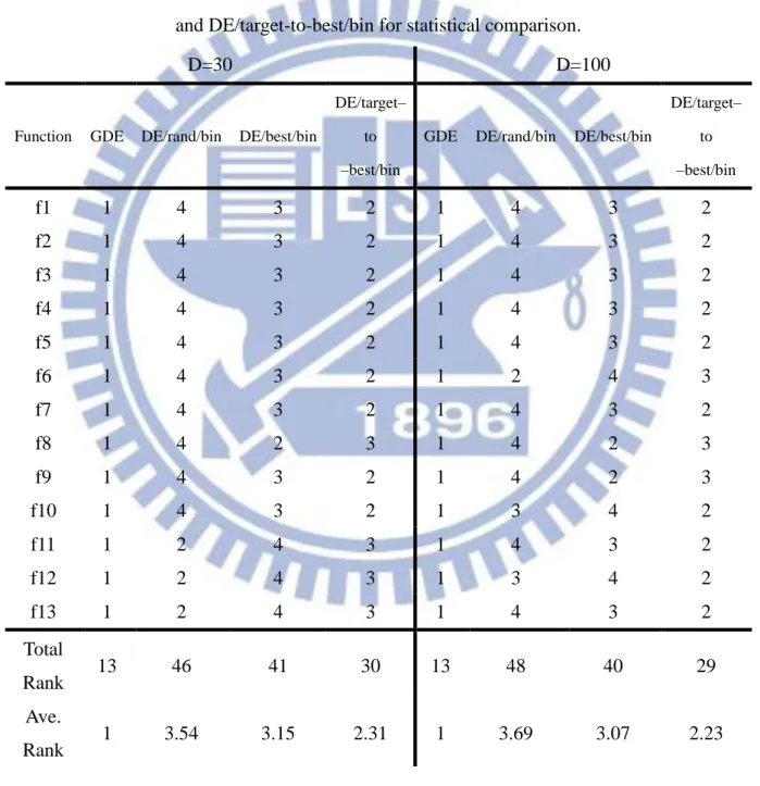
A rank relationship of the GDE, DE/rand/bin, DE/best/bin and DE/target-to-best/bin algorithms is shown in Table 3.5. In this simulation, j=4, T=13 and CD = 0.13. Table 3.6 presents a complete result of Friedman test. Under the 30 dimensional problems, all differences were greater than the critical difference, which means the GDE algorithm is signiﬁcantly better than the DE/rand/bin, DE/best/bin and DE/target-to-best/bin algorithms in this case. Under the 100 dimensional problems, the difference between the GDE algorithm and the DE/target-to-best/bin algorithm was smaller than the critical difference, which seems to suggest that the GDE algorithm is likely to be different from the DE/target-to-best/bin algorithm. However, in statistics theory, the Friedman test could not prove the significant difference between the GDE algorithm and the DE/target-to-best/bin algorithm. Otherwise, the proposed GDE algorithm was significantly better than the DE/rand/bin algorithm and the DE/best/bin algorithm in 100 dimensional problems. In this paper, an additional statistical test, called Wilcoxon signed-rank test [41], was performed for comparison with the GDE algorithm and the DE/target-to-best/bin algorithm in 100 dimensional problems. Finally, we obtain a P-value = 8.53×10-19. This result indicated that the GDE algorithm achieves

(48)

38

signiﬁcantly better performance than DE/target-to-best/bin algorithms in 100 dimensional problems. The overall result of Friedman test indicates the signiﬁcant difference between the proposed GDE algorithm and other methods for 100 dimensional problems and 30 dimensional problems.

Table 3.5: The rank table based on experimental results of GDE, DE/rand/bin, DE/best/bin and DE/target-to-best/bin for statistical comparison.

D=30 D=100

Function GDE DE/rand/bin DE/best/bin

DE/target– to –best/bin

DE/target– to –best/bin f1 1 4 3 2 1 4 3 2 f2 1 4 3 2 1 4 3 2 f3 1 4 3 2 1 4 3 2 f4 1 4 3 2 1 4 3 2 f5 1 4 3 2 1 4 3 2 f6 1 4 3 2 1 2 4 3 f7 1 4 3 2 1 4 3 2 f8 1 4 2 3 1 4 2 3 f9 1 4 3 2 1 4 2 3 f10 1 4 3 2 1 3 4 2 f11 1 2 4 3 1 4 3 2 f12 1 2 4 3 1 3 4 2 f13 1 2 4 3 1 4 3 2 Total Rank 13 46 41 30 13 48 40 29 Ave. Rank 1 3.54 3.15 2.31 1 3.69 3.07 2.23

(49)

39

Table 3.6: The result of Friedman test for statistical comparison. D = 30

Algorithm Difference in Rank Critical Difference(CD) DE/rand/bin (3.54－1) ＝ 2.54 1.30 DE/best/bin (3.15－1) ＝ 2.15 DE/target–to–best/bin (2.31－1) ＝ 1.31 D = 100 DE/rand/bin (3.69－1) ＝ 2.69 1.30 DE/best/bin (3.07－1) ＝ 2.07 DE/target–to–best/bin (2.23－1) ＝ 1.23 D = 30 & D = 100 DE/rand/bin (3.61－1) ＝ 2.61 0.91 DE/best/bin (3.11－1) ＝ 3.11 DE/target–to–best/bin (2.26－1) ＝ 1.26

3.3.5 Comparisons with Other Methods

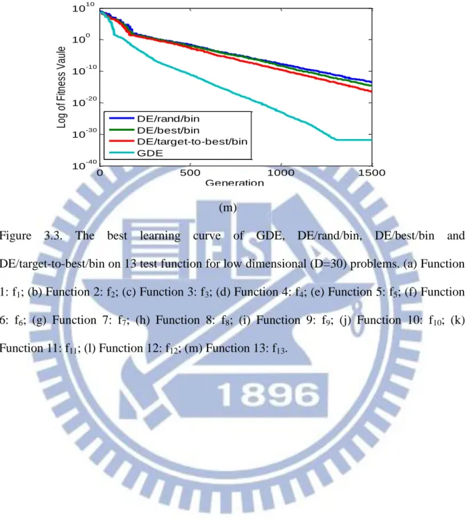
A further result of the GDE algorithm which compares with other evolutionary algorithms is presented in this section. Table 3.7 shows the comparison of the GDE algorithm and other evolutionary algorithms with 30 dimensional problems. These algorithms include RMEA[45],CEP[30], ALEP[43], BestLevy[43], NSDE[40] and RTEP[44]. The GDE algorithm obtained the best results on six out of eight functions. Table 3.8 shows the comparison of the GDE algorithm and advanced DE algorithms, including jDE[33,47], SaDE[26], ODE[27], SaCDE[16], DEGL[18] and JADE[22,46]. On unimodal

(50)

40

function problems (Function 1 –Function 6); the GDE algorithm obtained the best results on four out of six functions. On multimodal function problems (Function 7 –Function 13), the GDE algorithm obtained the best results on four out of seven functions and has a result near the best solution on f10. The overall results showed that GDE algorithm is a more effective

algorithm than other competitive algorithms.

Table 3.7: Comparison with the proposed GDE algorithm and other methods (D=30), including RMEA[45],CEP[30], ALEP[43], BestLevy[43], NSDE[40] and RTEP[44].

Function

GDE RMEA[45] CEP[3,44] ALEP[43] BestLevy[43] NSDE[40] RTEP[44] Performance

f1 1.83E–42 1.10E–17 9.10E–04 6.32E–04 6.59E–04 7.10E–17 7.50E–18

f3 1.13E–25 2.21E–15 2.10E+02 4.18E–02 3.06E+01 7.90E–16 2.40E–15

f7 3.73E–07 3.10E–04 8.60E+01 4.34E+01 5.77E+01 5.90E–28 1.10E+00 f9 5.68E–13 1.74E–08 4.34E+01 5.85E+00 1.30E+01 – 2.50E–14

f10 9.69E–15 5.08E–06 1.50E+00 1.90E–02 3.10E–02 1.69E–09 2.00E–10

f11 0.0E+00 6.41E–20 8.70E-00 2.4E–02 1.80E–02 5.80E–16 2.70E–25

f12 1.50E–32 1.72E–08 4.80E–01 6.00E–06 3.00E–05 5.40E–16 3.20E–13

分組式差分進化演算法及其應用於模糊系統最佳化設計

國

立

交

通

大

學

電控工程研究所

博

士

論

文