加入共變數於三元體資料分析以估計疾病基因位置

國 立 交 通 大 學

統計學研究所

碩 士 論 文

加入共變數於三元體資料分析

以估計疾病基因位置

Incorporating Covariates into Linkage-Disequilibrium

Mapping Using the Case-Parent Trio Design

研 究 生：李昱緯

指導教授：邱燕楓 博士

加入共變數於三元體資料分析

以估計疾病基因位置

Incorporating Covariates into Linkage-Disequilibrium

Mapping Using the Case-Parent Trio Design

研 究 生：李昱緯 Student: Yu-Wei Lee

指導教授：邱燕楓 Advisor: Dr. Yen-Feng Chiu

國 立 交 通 大 學

統計學研究所

碩 士 論 文

A Thesis

Submitted to institute of Statistics College of Science

National Chiao Tung University in Partial Fulfillment of the Requirements

for the Degree of Master

in Statistics June 2008

Hsinchu, Taiwan, Republic of China

中華民國九十七年六月

加入共變數於三元體資料分析

以估計疾病基因位置

研究生：李昱緯 指導教授：邱燕楓 博士

國立交通大學統計學研究所

摘要

Case-parent trio design 常被用在遺傳流行病學研究中，相較於其他的傳 統方法，例如：affected-sib-pair (ASP) sign，case-parent trio design 更 適合應用在罕見疾病。Liang 等人在 2001 年時根據 case-parent trio design 提出一種疾病基因相關定位的方法，他們利用偏好傳遞統計量(expected preferential-transmission statistic)估計疾病基因的位置。相較於傳統的 TDT 方法，他們指出，這個方法不但較有效力，且可以應用於更廣泛的資料。此 外，除了利用假設檢定去尋找疾病基因的位置，這個方法還能對疾病基因位點， 提供準確的估計值及其相對應的標準差，以對這疾病位置作推論。因為許多複雜 的疾病是由基因和環境因素的交互作用所造成，因此，加入這些基因或環境因素 於三元體的資料分析，應能對疾病基因位點，做更精準的定位。在本研究中，我 們用 case-parent trios 的資料，分別利用有母數和無母數的方法，將相關的 共變數併入模型中，以幫助我們估計疾病基因的位置。模擬結果和兔唇資料分析 均顯示，估計疾病基因位置時，加入共變數，會使得估計值更有效率。 關鍵詞：多點檢定; 連鎖不平衡; 三元體資料; 連續型變數; 有母數方法; 無母 數方法。

Incorporating Covariates into Linkage-Disequilibrium

Mapping Using the Case-Parent Trio Design

Student: Yu-Wei Lee Advisor: Dr. Yen-Feng Chiu

Institute of Statistics

National Chiao Tung University

ABSTRACT

Case-parant trio design is commonly used in genetic epidemiological family studies. It is more suitable for rare disorders than other conventional designs for family studies, such as affected-sib-pair (ASP) designs. Liang et al. (2001b) proposed a multipoint linkage disequilibrium (LD) mapping approach to localize disease genes based on a preferential-transmission statistic in the case-parent trio design. They found that their approach was more powerful and could accommodate a wider variety of data than the conventional TDT approach. In addition, instead of conducting hypothesis testing to search for a disease locus, it provided a precise estimate for a postulated disease locus along with its standard error, so that one can make inference for the disease locus. Most complex diseases involve both genetic and environmental components, incorporating genetic or environmental factors into the LD mapping may be helpful in localizing the disease locus. We therefore incorporated trait-related covariates into the LD mapping to estimate the disease locus through parametric and nonparametric models in the case-parent trio design in the present study. Simulation studies and the example of oral cleft study both suggested that incorporating covariates into the LD mapping approach helps a great deal to improve efficiency in localizing the disease locus.

Key words: Multipoint; Linkage disequilibrium; Case-parent trio design; Covariates; Parametric approaches; Nonparametric approaches.

誌謝

從口試委員的口中聽到了「恭喜」這兩個字時，內心的激動是不可言喻的。 回想起開始做論文時，對自己的能力總是存在著一些不確定感，所幸這一年來， 謝謝我的指導教授邱燕楓老師不僅一步步地引導我進入基因統計這門陌生的領 域，在每週一次的報告中也不厭其煩地解決我的疑惑、指正錯誤的觀念。雖然我 不能算是一個很認真的學生，但是您從不吝嗇在別人面前稱讚我，而您給我的鼓 勵也總是多過於責難，因為您認真嚴謹的要求才能讓這篇論文順利地誕生。 感謝所上的教授對我們的指導與照顧，讓我們在交大統研的這兩年內學到了 許多有用的知識；感謝最美麗的所辦小姐郭姐，常常在忙碌的工作之餘，還得傾 聽我們的苦水，認真的工作態度讓我們省去許多時間去處理學校生活上的瑣碎 事。當然也要感謝陪伴我這兩年生涯的好夥伴們，謝謝小爸不時給予我適時的安 慰與鼓勵，謝謝小胖廷常常傾聽我的抱怨給予我適當的建議，謝謝嗡嗡在我忙碌 之餘提醒我該吃飯了，謝謝小老婆提供許多在研究室的娛樂活動，謝謝重耕和彥 銘在我需要幫忙的時候毫不猶豫地伸出援手，謝謝小螞蟻經常幫我解決程式方面 的問題，謝謝小樹林帶給研究室許多歡樂，謝謝班代這兩年的辛苦，同時也謝謝 郃嵐、香菱、佩芳、姿蒨和鈺婷妳們的陪伴和照顧，特別感謝每天陪伴我超過十 二小時的許小雞總是不辭辛勞、不計代價地擔任我的司機和顧問。另外我想感謝 的是國衛院的徽宜學姊、君儀學姊和素梅學姊，妳們不只是幫助我解決論文和程 式方面的問題，對我的關心也讓我感到溫馨，能認識妳們是我進國衛院除了論文 以外最大的收穫。謝謝各階段和各方面的親朋好友，你們對我的鼓勵和祝福是我 完成論文最大的動力。此外，謝謝黃冠華老師、陳君厚老師和楊欣洲老師，感謝 您們不僅抽空擔任我的口試委員，並且在口試過程中給予我寶貴的意見和鼓勵， 讓我能更深入地去了解這領域的內涵和發展。 最後謹以此篇論文獻給我最愛的家人們，雖然奶奶沒辦法親眼看到我穿上碩 士服的那一刻，但我相信在天國的您還是會像以前一樣以我這孫子為榮。親愛的 爸媽、大姐佩芳、二姐衣樺和輝賓大哥，謝謝你們幫我解決許多生活上的雜事， 讓我可以毫無顧慮地專注在我的課業上，而且在我煩悶之餘帶我去郊外吹風散 心。也謝謝小舅和小舅媽對我的照顧與關心，因為你們的鼓勵我才能更有信心地 往自己的未來邁進。 李昱緯 于交通大學統計所 民國九十七年七月二日

Content

Abstract (in Chinese) ...i

Abstract (in English)...ii

Acknowledge (in Chinese)... iii

Content...iv

The List of Tables ...vi

The List of Figures... viii

1.

Introduction ...1

2.

Literature Review ...6

2.1 Transmission/Disequilibrium Test (TDT)...6

2.2 Extension of TDT from one marker to multiple markers ...7

2.3 Extension of TDT from bi-alleles marker to multiallele marker ...10

2.4 Extension of TDT from trio data to affected sib pair data ...12

2.5 Extension of TDT without parents’ data ...13

2.6 Extension of TDT from qualitative traits to quantitative traits...15

2.7 Localization of disease locus in case-parent trio designs ...17

2.8 Multipoint approach with covariate data ...18

2.9 Multipoint approach with covariate data and non-parametric approaches ....18

2.10 Interpreting analyses of continuous covariates in ASP...20

3.

The Proposed Method...22

3.1 Notation and Preferential-Transmission Statistic...22

3.2 The Parametric Approach with Covariates ...24

3.3 The Nonparametric Approach with Covariates...26

4.

Simulation Studies...29

4.1 Disease models...29

4.1.1 Logistic regression models ...29

4.1.3 Fixed penetrance models...31 4.2 Genotype Data ...32 4.3 Simulation Results ...33

5.

A Data Example...39

6.

Discussions ...42

References...44

The List of Tables

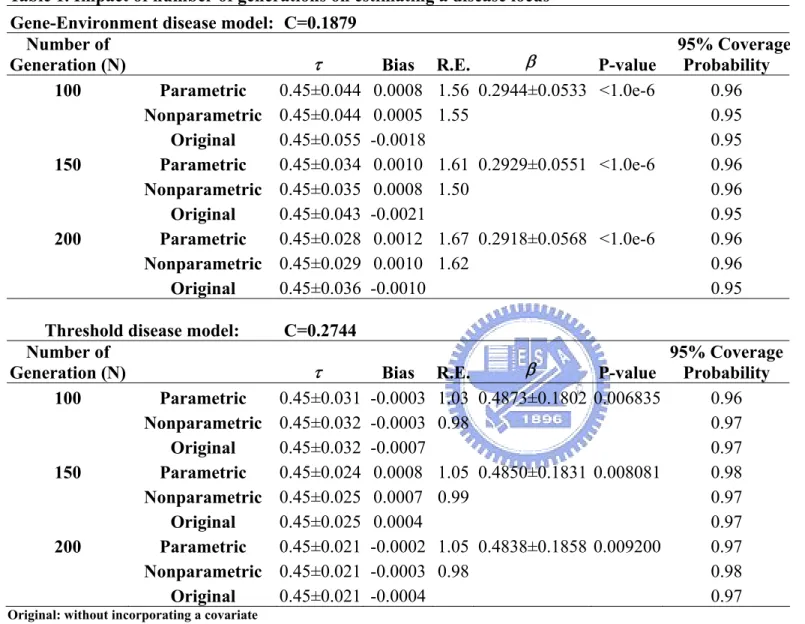
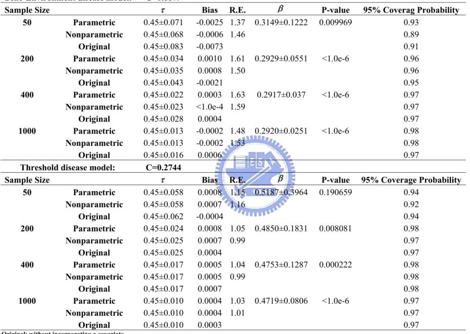
Table 1. Impact of number of generations on estimating a disease locus

...48

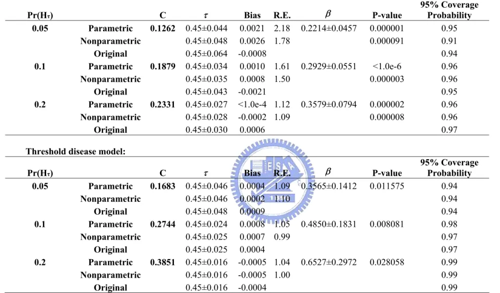
Table 2. Impact of disease allele frequency on estimating a disease locus

...49

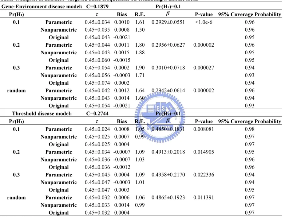
Table 3. Impact of sample sizes on estimating the disease locus...50 Table 4. Impact of markers’ targeted allele frequencies on estimating a

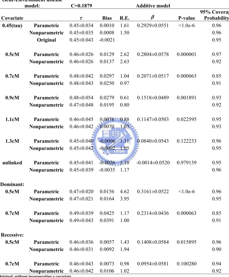
disease locus ...51 Table 5. Impact of markers’ density on estimating a disease locus

(τ=0.45 with 10 markers, τ=0.475 with 20 markers)...52 Table 6. Impact of ε on estimating a disease locus...53

Table 7. Impact of β₀(the risk of referent population) on estimating a

disease locus ...54

Table 8. Impact of β₁ and β₂ (genetic effect) on estimating a disease

locus ...54

Table 9. Impact of β₃ (environment effect) on estimating a disease

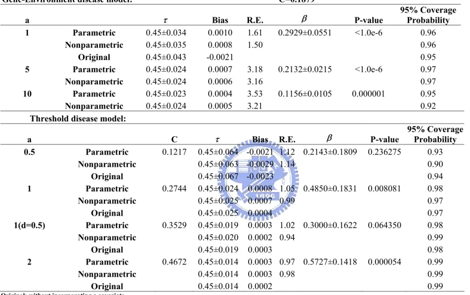
locus ...55 Table 10. Impact of the additive genetic effect “a” on estimating a

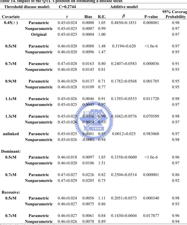
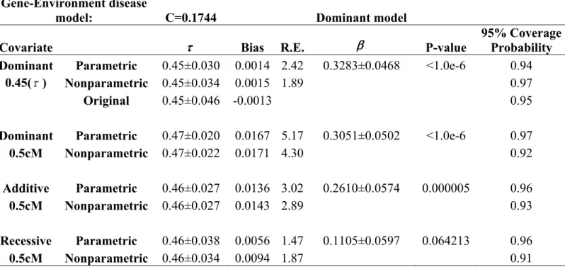
disease locus ...56 Table 11. Impact of prevalence rates on estimating a disease locus ...57 Table 12. Fixed penetrance disease model ...57 Table 13. Impact of the QTL’s position on estimating a disease locus..58 Table 14. Impact of the QTL’s position on estimating a disease locus..59 Table 15. Impact of the QTL’s position and genetic models of the

quantitative trait on estimating a disease locus...60 Table 16. Impact of the QTL’s position and genetic models of the

quantitative trait on estimating a disease locus (with an underlying recessive model)...60 Table 17. Impact of the QTL’s position and genetic models of the

quantitative trait on estimating a disease locus (with an underlying dominant model)...61 Table 18. Impact of the QTL’s position and genetic models of the

quantitative trait on estimating a disease locus (with an underlying recessive threshold model)...61 Table 19. Impact of the genotype τ on estimating β ...62

Table 20. The proportions of each covariates’ category for probands recruited from four populations from the oral cleft study ...63 Table 21. Incorporating different covariates for four combined

populations (Korea, Maryland, Singapore, and Taiwan) from the non-syndromic oral cleft study...64 Table 22. Incorporating different covariates for Korean population

from the non-syndromic oral cleft study...65 Table 23. Incorporating different covariates for population in

Maryland from the non-syndromic oral cleft study...65 Table 24. Incorporating different covariates for Singaporean

population from the non-syndromic oral cleft study ...66 Table 25. Incorporating different covariates for Taiwanese population

from the non-syndromic oral cleft study...66 Table 26. Incorporating different covariates for Korean and Taiwanese

The List of Figures

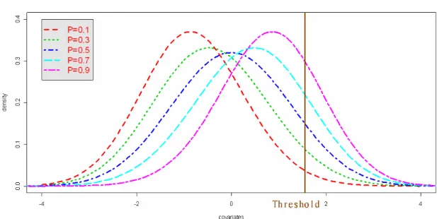
Figure 1. Graphical illustration of logistic regression disease models ..30 Figure 2. Graphical illustration of threshold disease models...31 Figure 3. Disease allele frequencies and the probability density function

for a covariate in the threshold models (P=disease allele frequency, a=1, d=0) ...31 Figure 4. Graphical illustration of fixed penetrance disease models ....32

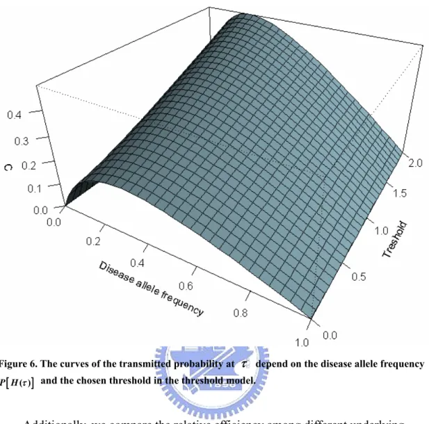
Figure 5. The curves of the transmitted probability C at τ depend on

the disease allele frequency P H_[ ( )τ _] with penetrance rates f0=0.491, 1 0.153

f = , and f₂=0.022 in the logistic regression disease model. ...34

Figure 6. The curves of the transmitted probability at τ depend on the

disease allele frequency [P H( )τ ] and the chosen threshold in the

threshold model. ...35 Figure 7. True, observed and fitted curves by the original approach, the

proposed parametric approach and the proposed nonparametric

approach...68 Figure 8. The transmitted statistic from 2.7 cM to 175 cM on

chromosome 4p16 from oral clefts data (Sull et al. 2008)...68 Figure 9. The transmitted statistic from 3 cM to 7 cM on chromosome

4p16 from oral clefts data (Sull et al. 2008) ...69 Figure 10. The transmitted statistic from 4 cM to 6 cM on chromosome

4p16 from oral clefts data (Sull et al. 2008) ...69 Figure 11. The transmitted statistic from 4.5 cM to 5 cM on

chromosome 4p16 from oral clefts data (Sull et al. 2008)...70 Figure 12. The transmitted statistic from 4.65 cM to 4.75 cM on

chromosome 4p16 from oral clefts data (Sull et al. 2008)...70 Figure 13. Comparisons of three approaches by incorporating gender

into the LD mapping ...71 Figure 14. Comparisons of three approaches by incorporating affected

father into the LD mapping...71 Figure 15. Comparisons of three approaches by incorporating affected

mother into the LD mapping...72 Figure 16. Comparisons of three approaches by incorporating smoking

into the LD mapping ...72 Figure 17. Comparisons of differences in incorporating population

types or drinking in the parametric approach ...73 Figure 18. Comparisons of three approaches by incorporating gender

into the LD mapping ...73 Figure 19. Comparisons of three approaches by incorporating drinking

into the LD mapping ...74 Figure 20. Comparisons of three approaches by incorporating gender

into the LD mapping ...74 Figure 21. Comparisons of three approaches by incorporating smoking

into the LD mapping ...75 Figure 22. Comparisons of three approaches by incorporating drinking

into the LD mapping ...75 Figure 23. Comparisons of three approaches by incorporating vitamin

into the LD mapping ...76 Figure 24. Comparisons of three approaches by incorporating gender

into the LD mapping ...76 Figure 25. Comparisons of three approaches by incorporating gender

into the LD mapping ...77 Figure 26. Comparisons of three approaches by incorporating drinking

into the LD mapping ...77 Figure 27. Comparisons of three approaches by incorporating gender

into the LD mapping ...78 Figure 28. Comparisons of three approaches by incorporating smoking

into the LD mapping ...78 Figure 29. Comparisons of three approaches by incorporating drinking

1. Introduction

Case-parent trio design is commonly used in present genetic epidemiology. It is more suitable for rare disorders than other conventional designs, such as

affected-sib-pair (ASP) designs. In addition, the trio design does not require multiplex siblings needed in ASP designs. For trio data, the method named

Transmission/disequilibrium test (TDT) (Spielman et al. 1993) was proposed to detect linkage when a disease-susceptibility locus is found to be associated with a marker in family triads, including two parents and one affected child. Risch and Merikangas (1996) proved that TDT is more powerful statistically to test genes of modest effect than ASP designs, even in the presence of population stratifications.

Many extended methods of TDT were proposed in recent year to deal with more complex situations. For example, (i) TDT without parents marker data—Sib-ship disequilibrium test (SDT) (Horvath and Laird, 1998) and Sib

transmission/disequilibrium (S-TDT) (Spielman et al. 1998). These two methods exploited one or more unaffected siblings’ marker data instead of parents’ marker data that may be absent. The defect is that these methods are not as powerful as TDT, so they are only adaptable when lacking parents data; (ii) TDT with pedigree data— pedigree disequilibrium test (PDT) (Martin et al. 2000) can catch extra information from general pedigrees out of original trio data regardless of their size and obtains a valid TDT even when there is misclassification of unaffected individuals, especially with a high-prevalence model; (iii) TDT with multi-allele markers. (Bickeböller and Clerget-Darpoux 1995, Sham and Curtis 1995; Terwilliger 1995; Schaid 1996; Spielman and Ewens 1996; Cleves et al. 1997; Kaplan et al. 1997; Lazzeroni and Landge 1998), Sham and Curtis (1995) proposed an extension of

transmission/disequilibrium test for dealing with multi-allele problem, but the approach has good power only when linkage disequilibrium is strong and the disease

is recessive. On the other hand, Spielman and Ewens (1996) also revised their biallelic TDT to muiltiallelic TDT; and (iv) TDT with multiple markers (Terwilliger 1995; Lazzeroni and Landge 1998; Clayton and Jones 1999; Clayton 1999; Dudbridge et al. 2000). Zhao et al. (2000) also proposed a new approach about multiple markers and corrected the disadvantage of prior approaches. (E.g. Lazzeroni and Landge’s approach ignores the dependence of marker, Clayton’s approach is not robust to population stratification, and for Dudbridge’s approach, ambiguous haplotypes have to be discarded.) In solving the problem of unknown haplotype frequency, it is important and bounden to know the information of parents’ genotype. Besides, although haplotype with multimarker is more informative than single marker, it also results in a larger number of degrees of freedom and reduces the power of these tests simultaneously. The new approach-- Haplotype-sharing TDT (HS-TDT) (Zhang et al. 2003), not only remains informative as traditional haplotype-based tests, but decreases the degrees of freedom. HS-TDT is applicable to both qualitative and quantitative traits, arbitrary size of nuclear family with or without ambiguous phase information, and whatever number of alleles at each marker. However, Knapp et al. (2004)

declared that if the genotyping error exists, even the probability of genotyping errors is low, HS-TDT cannot have a precise type I error.

Although the original TDT was powerful and robust, it could not include the informative trait or covariate. In earlier research, Haseman and Elston (1972) used sib pairs’ data, not trios’ data we required in TDT, to estimate linkage between a known marker with malleles and a susceptibility disease locus which governs a quantitative trait with biallelic genotype. Many other researchers developed a lot of extended methods for dealing with quantitative-covariate with IBD (e.g. Sham et al. 2002). Recently, some researches devoted on connecting TDT and a quantitative or

et al. 2000, 2002; Liang et al. 2001; Wheeler and Cordell, 2007), such as QTDT (Rabinowitz 1997; Lunetta et al. 2000). QTDT makes use of quantitative phenotype as a dependent variable, which improved and redefined quantified genotype as an independent variable to generate linear regression. In addition, Hierarchical QTDT (HQTDT) (Fulker et al., 1999) separates genotype (independent variable) by different mating-type-- QTDT_M(Gauderman, 2003) utilized the information of mating-type instead of the intercept of original regression model, and in Retrospective QTDT (RQTDT), the genotype is modeled as a function according to their phenotype and the parental genotypes (Liu et al. 2002). Gauderman (2003) employed above tests to detect three effect, genetic main effect, gene-environment interaction effect, and gene-gene interaction effect. After that, he found QTDTMis more efficient (i.e.

required less sample size) than other tests under the necessary condition that the all genotypes of markers of trios data should be known, but it is not realistic.

In multipoint linkage analysis using affected sib pairs, Liang et al. (2001a) capitalized upon IBD information of multiple markers around a susceptibility gene and then obtained a simple formula between the expected numbers of allele-sharing of these markers and the susceptibility gene by careful assumption and complicated calculation. According to the formula, they applied generalized estimating equation (GEE) method (Liang and Zeger 1986) to estimate all parameters (including the disease location τ ) in the model and variances of the estimates at the same time. The parameter C represents estimated expected number of allele-sharing of τ , and the range of value is from -1 to 1. The magnitude (absolute value) of parameter C in their method indicates the ability of estimating the true location of susceptibility gene. The advantage of this approach is that it did not require specification of penetrance or a mode of inheritance.

allele-transmitted information of trio data instead of allele-sharing information of sibling data, and rewrote the formula between information of markers and the parameter C for case-parent trios data. In the traditional TDT method, only

heterozygous parent data are informative and could be included, but in Liang et al.’s model, homozygous parent data could be recruited simultaneously. Furthermore, they could test if there is linkage or linkage disequilibrium between a disease gene and multiple genetic markers over the region at the same time, which is not like the conventional TDT where each marker－ is tested separately resulting in a multiple testing problem. Specially, the method is not restricted to trio designs only, it can also be extended for other types of data. On the other hand, the approach of Liang et al. is usually more powerful than the traditional TDT approach (Liang et al. 2001b).

Glidden et al. (2003) quoted Liang’s formula for ASP designs (2001a) and added age-at-onset information as a covariate to support the estimation of parameter C. The information of covariates can yield substantial efficiency gains on finding the location of susceptibility gene. Chiou et al. (2005) also adopted Liang’s formula in ASP

designs (2001a), they utilized nonparametric approach to model and estimate C as a function of covariates at first, and then applied the GEE method to estimate the

location of τ . By an iterative process, the estimation of C and τ could be obtained until convergence was reached. According to Chiou et al. (2005), the nonparametric method is better than the quadratic and linear models, because the nonparametric method avoids the flaw of using misspecified parametric regression models. Under case-parent trio designs, we propose a new multipoint approach for estimating the location of a susceptibility gene, τ. The proposed approach is based on transmission information of markers near an unobserved disease gene and a quantitative or a qualitative covariate associated with the disease gene. We model C as a function of covariates through parametric and nonparametric approaches, so as to

incorporating covariates into the association mapping in estimating the location of susceptibility locus τ.

2. Literature Review

2.1 Transmission/Disequilibrium Test (TDT)

The transmission/disequilibrium test (TDT) can be utilized if a heterozygous parent transmits his or her target allele and alternative allele to affected child with equal frequency. It only requires affected children of trio data rather than multiple affected or unaffected family members. Besides, it detects the linkage between susceptibility gene and marker locus when association is present.

Consider two bi-allelic (a target allele D and a normal allele ₁ D ) markers ₂

1

M and M , and suppose there have ₂ n trio families which have two parents and

an affected child. After collecting this type of data, researchers arrange 2n parents of trio data into a 2 2× table shown in the Table 2 in Spielman et al. 1993.

1 2

1

Nontransmitted Allele Transmitted Allele M M Total M 2 M Total a b a b c d c d a c + + + b+d 2 n

The above table shows every parent’s genotype and the alleles which he or she transmits and does not transmit to affected child. Then, they assume a coefficient δ represents linkage disequilibrium (- freq(M D )_{1 1} − mp , m and p are the population frequency of allele M and ₁ D ), and ₁ θ represents the recombination

fraction between marker M and locus D. With these coefficients, the Table can be rewritten as the Table 3 in Spielman et al. 1993:

Nontransmitted Allele Transmitted 1 2 Allele M M Total

[

]

[

]

2 1 2 M ( / ) (1 ) (1 ) / (1 ) / M m + mδ p m −m + − −θ mδ p m+ −θ δ p

[

]

2

[

]

[

]

(1 ) ( ) / (1 ) (1 ) / 1 (1 ) / Total ( / ) 1 ( / ) 1 m m m p m m p m p m p m p θ δ δ θ δ θδ θδ − + − − + − − − − + − −

The null hypothesis is that there is no linkage (θ =1 / 2), it also represents

( ) ( )

E b = E c whatever the value of m and p , but the necessary condition is that the value, δ , should not be zero. On the other word, a heterozygous parent transmits

target allele and normal allele with equal frequency. Under the null hypothesis, we suppose b is distributed in binomial distribution with b+c sample sizes, which are the total numbers of heterozygous parents, and the probability is 1/2.

1

2 2 4

~ ( , ) ( ) b c, ( ) b c .

b Binomial b c+ ⇒E b = + Var b = +

Under this hypothesis, the _χ2 _{statistic has the form (McNemar’s test, Sokal and} Rohlf, 1969)

(

)

2 2 2 2 4 (b b c) b c b c . b c χ =⎛⎜_⎜ − + + ⎞⎟_⎟ = − + ⎝ ⎠

The TDT is often more powerful than other conventional linkage tests and it is not affected by population structure which can lead association in the absence of linkage, since it exploits within-family comparisons only. Although TDT is much more sensitive than traditional haplotype sharing test (Risch and Merikangas 1996), and only requires a single affected child, it should be utilized under the existence of population association, even the linkage is strong.

2.2 Extension of TDT from one marker to multiple markers

Since the Human Genome Project is progressing rapidly, the genetic marker can be identified and genotyped easily and that can help us to acquire more information. After the information of multiple markers is obtained easily, many researchers proposed relative tests. We will introduce some existing and known methods below.

Lazzeroni and Lange (1998) analyzed each marker separately and obtained the adjusted P -value which is the minimum of P -values under the null hypothesis that there is no linkage between the region over each markers, but it ignored the

dependence which may result in linkage between markers.

Some researchers use the haplotype instead of the information of multiple markers, and assume the haplotype of parents and affected child are known. Clayton

(1999) estimated the frequency of haplotype and calculated the likelihood after considering all possible solutions, but it is not robust when population stratification is present. Dudbridge et al. (2000) proposed an unbiased TDT for individual haplotype, they calculated the correct variance of the transmission count within family, and used extra information from multiple siblings if they are available. Similar to Clayton’s work, they utilized missing data techniques to estimate the uncertain haplotype, so this method is also not robust when population stratification is present. To avoid this kind of problem, some family data with equivocal haplotype should be discarded, but it discards a part of information simultaneously.

Under knowing all haplotype information of each parent, Zhao et al. (2000) displayed a h h× transmission/nontransmission table T as

11 12 1 21 22 2 1 2 1 2 1 2 h h h h hh h t t t t t t h t t t ,

where t is the number of parents with haplotypes _ij H H and they transmit H_{i j γ} to

the affected child but not transmit H_δ, where h is the total number of possible haplotype. After completing this table, they can calculate a statistic:

(

)

2 . . 1 . . 1 . 2 h t t h T h t t t γ γ γ= γ γ γγ − − = + −

∑

The statistic is a marginal homogeneity test, since it may not approximate a _χ2 distribution with h−1 degree of freedom, we can use simulation methods to assess the P -value. With ambiguous parents’ haplotype, they detected T (estimating _ml

haplotype frequency by assuming that parents are random samples of individuals from population under Hardy-Weinberg equilibrium), which has the highest power than T _u

(estimating haplotype frequencies by making use of both unambiguous families and ambiguous families, and assigning each compatible haplotype group equal probability for each ambiguous family). Furthermore, testing each marker separately and

discarding the ambiguous families have lower power.

Although the approach using multiple markers is more informative than using a single marker, there exists some difficulties. For example, if we consider each haplotype as an allele in TDT, the degree of freedom will increase rapidly according to the number of markers and then result in lower power. On the other hand, the haplotype of parents are not always unequivocal. Zhang et al. (2003) proposed a haplotype-sharing TDT (HS-TDT) which utilized the similarity of haplotype as the information. Let _, ( )

i j

H H

S l be the distance between the leftmost and the rightmost

markers with identical alleles l (See figure 1 of Zhang et al.). For any haplotype H , the score of lth marker is defined as

4 , 1 1 1 ( ) ( ), 4 ij n H H H i j X l S l n = = =

∑∑

where H is four kinds of parental haplotypes in the ij i

th _{family. Then let} 4

1 ( )

ik _j ijk ij

x =

∑

₌ ξ X l be the difference of the haplotype-sharing score between the

transmitted parental haplotypes and non-transmitted parental haplotypes, ξijk= 1 means the haplotype Xij( )l transmitted to k

th _{child and} ijk

ξ = -1 means the

haplotype Xij( )l is not transmitted to k

th _{child. They estimated the covariance} between the value of trait y (for the qualitative case, _ik y = 1 means the child is _ik

affected, and y = 0 means the child is not affected, for the quantitative case, _ik y _ik

can represent the quantitative value directly.) and the transmitted score x , _ik

( ) i ( ) ( ),

t

i ik ik

where c can be arbitrary constant, Zhang et al. (2003) set it as the average of trait value over all children. Under the null hypothesis of no linkage and association,

[

i( )

]

E U l is equal to zero for any value of c. We can find that if the disease

mutation causes high trait value, the value of U l should be positive. Similarly, if _i( )

the disease mutation causes low trait value, the value of U l should be negative. _i( )

Let ( ) n₁ ( ) i i i

U l =

∑

₌ w U l , where w_i > is a weight function over each family and 0

the statistic of HS-TDT is defined by 1 max ( ) , l L U U l ≤ ≤ =

where L is the total number of markers. It is noticeable that the choice of c and w _i

will influence the power of test. Finally, they utilized the permutation procedure to evaluate the P -value of test.

HS-TDT is applicable to both qualitative and quantitative traits, it decreases the degree of freedom with traditional haplotypes method, it has correct false-positive error rate, and it is more powerful than single-marker TDTs and haplotype-based TDTs.

2.3 Extension of TDT from bi-alleles marker to multiallele marker

A biallelic marker is assumed under traditional TDT method, but sometimes many markers over chromosome of human have more than two alleles, such as blood type which has A, B, and O, three alleles basically. So when TDT is introduced and popular over the world, some researchers devoted to extending TDT to multiallele marker. The original approach, generalized TDT (Bickeböller and Clerget-Darpoux, 1995), is to combine HHRR (haplotype-based haplotype relative risk) statistic (Terwilliger and Ott, 1992) and TDT:

(

)

2 ij ji c i j ij ji t t T t t < − = +

∑

,

where t is the number of parents who transmitted allele _ij i and not transmitted allele j . The statistic has asymptotically a _χ2 _{distribution with ( 1) 2}

m m− D.F. under the absence of linkage. But under the null hypothesis (θ =1 2) and the

presence of linkage disequilibrium, the statistic is invalid and has lower power, since the transmitted and non-transmitted allele are not independent. In addition to the test

c

T described above, they also proposed another statistic,

(

)

(

)

2 1 , t i i m i i i t t T t t ⋅ ⋅ = ⋅ ⋅ − = +

∑

where t_i⋅ and t_⋅i are the row and column marginal totals. The statistic is an

extension of the discussion of Ewens and Spielman (1995) for biallelic markers. Sham and Curtis (1995) proposed an extended method of TDT. First, they

calculated the probability (P ) of each type of transmitted and non-transmitted alleles _ij

conditional on parental genotype. Under θ = 0, ln(P_ij P_ji)= −b_i b_j, so there are

1

m− independent parameter b which related to the marker alleles _i M . For _i

convenience, b is set to zero, and then they define a likelihood ratio statistic by _m

2 0 1 2 ln*( ) ~ ( 1), l L T m L χ = − −

where L is the likelihood under null hypothesis that ₀ b = 0 for all _i i, and L is ₁

the maximized likelihood with respect to b . Then, they utilize the statistic to test if _i

there is linkage in the presence of linkage disequilibrium. They pointed out this approach has good power when linkage disequilibrium is strong if the disease is recessive.

marker:

(

)

2 2 1 1 ~ ( 1). 2 m i i mhet i i i ii t t m T m m t t t χ ⋅ ⋅ = ⋅ ⋅ − − = − + −

∑

Kaplan et al. (1997) compared these tests mentioned above and applied Monte Carlo test to guarantee valid tests and then concluded that T has the lowest power _c

than other three tests (T ,m Tmhet, and T ), and the three tests almost have similar l power over all situations (the variation of recombination fraction θ , and the different disease model) and population they classified.

2.4 Extension of TDT from trio data to affected sib pair data

When considering the case of families with two affected children, Spielman et al. (1993) provided three categories to define the information from heterozygous parents by 1 2 2 2 ,

i number of parents who transmit M to both children

j number of parents who transmit M to both children

h i j number of parents who transmit M to one child and M to the other

= = − − =

where h is the number of heterozygous parents, and then they rewrote the parameters b and c of TDT as 2 ( ) . 2 ( ) b i h i j c j h i j = + − − ⎧ ⎨ = + − − ⎩

By this definition, the TDT statistic could be written as 2 2( ) . i j TDT h − =

They also proposed other statistics for families with more than two affected offspring. Martin et al. (1997) devised a statistic with ASP data, and called the statistic T . _sp

Among children of heterozygous parents, let n be the number of ASPs who all ₁₁

allele M , and let ₂ n be the number of ASPs who one accepted ₁₂ M and the other ₁

accepted M . Then, the statistic would be ₂

(

)

2 11 22 11 22 . sp n n T n n − = +

Wicks (2000) simulated two tests (TDT and T ) and pointed out that sp T is valid sp when testing for both linkage and linkage disequilibrium, while TDT is only valid when testing for linkage, but not linkage disequilibrium. However, TDT is more powerful than T since TDT utilizes excess sharing—that is the tendency for sp

11 22

n +n exceeding n as linkage is present. Wicks also defined a general TDT-like ₁₂

statistics for ASPs as

(

)

(

)

2 11 22 11 22 12 ( ) ,0 1. (1 ) n n T n n n α α α α − = ≤ ≤ − + +

We can observe that T and TDT are the special case for _sp α = 0 and α= 1 2,

respectively. He found T(1) is most powerful test for detecting linkage and it has the

correct asymptotic false-positive error rate under the null hypothesis, since the statistic (1)T exploits excess sharing to the fullest extent possible.

2.5 Extension of TDT without parents’ data

Traditional TDT method required marker information of trio data, included an affected child and his or her parent, but in some late onset, such as cardiovascular, non-insulin-dependent diabetes, and other age related diseases, it’s difficult to know that. To handle this form of problem, some researchers tried to reform TDT method, for example, sib transmission/disequilibrium (S-TDT) (Spielman et al. 1998) and sibship disequilibrium test (SDT) (Horvath and Laird, 1998). They all utilized the marker data of unaffected sibs instead of parents.

The S-TDT determines if the marker allele frequency is different between affected offspring and their unaffected sibs significantly. It has two procedures, one is the permutation procedure, it can calculate the P -value that tests if the number of interested allele M is randomly arrange in affected and unaffected groups, but it ₁

needs sufficiently large number of replicates to keep a precise P -value . The other one is a Z-score procedure; it utilizes the hypergeometric distribution to estimate the expected mean U and variance V of interested allele M , and calculates the Z ₁

score, (Y U) Z V − = ,

where Y is the observed number of M , or the Z score with a continuity correction ₁

as 1 (Y U ₂) z V − − ′ = ,

and then the P -value can be calculated by normal distribution approximation. They also combine the TDT and the S-TDT by assuming the expected mean and variance of TDT, 2n and 4n , respectively, and adding them with expected mean and variance

of S-TDT. Lastly, we can calculate the combined Z score and corresponding

P -value.

The formula of S-TDT is similar with the Mantel-Haenszel test (Laird et al. 1998). It is noticeable that if we have the information of parent, we should choose TDT rather than S-TDT, because under such circumstance, TDT is more powerful than S-TDT. Although S-TDT is useful when the parent data are missed, it has some restriction: (1) the sibship must have at least one affected and one unaffected member; and (2) in the sibship, all members should not have the same genotype. Another method, SDT, is a nonparametric sign test. First, it denoted the mean number of target

allele among affected ( 1

A

m ) and unaffected (m ) siblings as _U1

A U

(total number of target alleles among the affecteds)/n (total number of target alleles among the unaffecteds)/n

T A T U m m = = ,

where n and A n are the total number of affected and unaffected members in the U sibship. They denoted the difference of T

A

m and m by _UT d , let T b be the number

of T

d > 0, and let c be the number of d < 0, so the statistic of SDT can be defined T

by the form of TDT. The two tests have similar power in most situations, but SDT is better than S-TDT, because it avoids accounting for correlation between the siblings, and it’s relatively simple. Similar to S-TDT, SDT can also combine with TDT by

SDT TDT

b = +b b , and c_SDT = +c c_TDT.

2.6 Extension of TDT from qualitative traits to quantitative traits

Due to the increasing availability of genetic data, many quantitative traits are noticed and related with susceptibility gene. At the start of research, one might related the phenotype and genotype with linear regression model:

,

i α βGi ei

ϒ = + +

where ϒ is the quantitative phenotype and _i G is marker’s genotypes, and then we _i

can test if the value of β equals to zero.

QTDT is proposed by Rabinowitz (1997), the linear regression model was revised as

i α βZi ei

ϒ = + +

where Z_i =H_im(T_im−1 2)+H_if(T_if −1 2), H_im(H_if) is an indicator of

heterozygosity in the mother (father), and T_im(T_if) is an indicator of that if the

mother (father) transmits a target allele to affected child. Furthermore, Lunetta et al. (2000) rewrote the QTDT,

(

| ,

)

.

i α β Gi E Gi gim gif ei

ϒ = + − ⎡_⎣ ⎤_⎦ +

Fulker et al. expanded the linear model to partition the covariate into between- and within- mating type information, two variables. They called the approach hierarchical QTDT (HQTDT) which has the form

( ) ,

i α βBGM βW Gi GM eM ei

ϒ = + + − + +

where e is a mating-type specific residual and it is assumed to be _M N( , )0τ2 , G _M

is some average genotype for mating type M . The test of association is based on an LRT of β_W.

On the other hand, the value of ϒ in the original QTDT model is restricted to

α , regardless of the mating type, so Gauderman (2003) proposed a reformatory method, QTDT , _M

.

i αM βGi ei

ϒ = + +

The difference from other models is that the extra term α_M considers the different effect of 6 mating type.

The models described above are all prospective, but there are some other models that are retrospective, such as retrospective QTDT (RQTDT) (Liu et al. 2002), which lets the genotype of affected children be modeled as a function conditional on their phenotype and their parental genotypes. Then, by Bayes rule, the likelihood becomes

(

)

(

₍

)

₎

1 * * *| , | , , , Pr( | , ) , , | , , , Pr( | , ) im if N i i i im if i _{i im if} g g g f G g g g L f G g g g α β σ α β σ α β σ = ϒ = ϒ

∏ ∑

,

where _σ2 _{is the residual variance. The summation in the denominator includes four} genotype ( *

g ) and it could be transmitted to a child conditional on parental

genotypes.

Gauderman (2003) compared these models under genetic main effects, gene-environment interaction, and gene-gene interaction, and then pointed out

M

QTDT needs less sample size than other models for testing these effects, i.e.

M

QTDT is the most efficient approach.

2.7 Localization of disease locus in case-parent trio designs

Liang et al. (2001b) applied the conception of TDT and developed a new statistic

( )

Y t , called the preferential- transmission statistic (It would be described in more

detailed in Chapter 3). Through complicated calculation, they showed the relationship between ( )Y t and ( )Y τ , the preferential-transmission statistic with arbitrary marker

and susceptibility gene’s locus, respectively is:

[

( ) |

]

(1 2 _, )

[

( ) |

]

(1 _, )N

{

Pr ( ) | ( )

[

]

}

t t

E Y t Φ = − θ _τ E Y τ Φ −θ _τ h t hτ ,

where Φ represents the event that the offspring of trio is affected, θt_,τ is the recombination fraction between marker locus t and the postulated disease gene location τ , and N is the number of generations since the introduction, into the population, of a disease-causing mutation at location τ .

Finally, they applied the generalized-estimating-equation (GEE) (Liang and Zeger, 1986) to estimate the parameter δ = ( , , )τ C N .

The approach can test the null hypothesis that there is no linkage or linkage disequilibrium (LD) to the region R by testing if C ≡0. In contrast to TDT, Liang et al.’s approach simultaneously uses all the markers’ information, so it is more powerful than TDT. The approach uses the data of every marker over the specific region regardless of whether the parent’s genotype is heterozygous or homozygous, and also provides valid standard-error estimates of parameter through GEE. Most of all, there is no need to assume the genetic model of the disease in this approach.

2.8 Multipoint approach with covariate data

Liang et al. (2001a) also proposed a multipoint approach with affected sib pair (ASP) data by the model as follows.

{

}

_{1 1 2} 2

{

}

₁

,

( ) | ( _t ) , ( ) | ,

E S t Φ = + − θ _τ C C = E S τ Φ −

where ( )S t and ( )S τ represent the number of alleles shared identical-by-descent

(IBD) at a marker locus t and a susceptibility locus τ , respectively. Glidden et al. (2003) incorporated age as a covariate X into the model of Liang et al. and assume

C is a function of covariate X . Their model has the form

{

}

(

)

2 1 1 2 1 0 04 , ( | ) ( ) | , ( ) ( ) exp . ( ). t t x E S t X x C x t C x τ μ θ τ = = Φ = + − = + − −

Furthermore, since the value of C is -1 to 1, it could be transformed and postulated as a logistic formula:

{

1 2

}

logit ( ) / T C x α β x ⎡ + ⎤= + ⎣ ⎦

Then, we could utilize GEE method to estimate the parameters, δ =( , , ,...,τ α β₁ β_p). Conclusively, they find incorporating covariate data could provide more

information, increase precision in localizing susceptibility gene and other parameters, and minimize the effect of the unknown heterogeneity process, even when it is mismodelled.

2.9 Multipoint approach with covariate data and non-parametric approaches

Although multipoint linkage analysis using sibpair designs is a popular approach to test the location of interested trait, some issues, such as genetic heterogeneity, gene-gene, and gene-environment interaction, should be addressed properly. Chiou et al. (2005) proposed an approach which assumes trait locus’ genetic effect is a function of covariate, and the function represents the probability of a sibpair sharing the same

allele at the trait locus. Then, they estimated the susceptibility gene locus with GEE method and the genetic effect with a nonparametric approach iteratively.

For the jth marker and ith sibpair, they applied Liang et al.’s (2001a) model and rewrote it as

{

}

2 1 2 1 1 2 _, ( ) | ( ) ( , ) j i j t i i E S t Φ = + − θ _τ C x x

Let g=( ( ,g x x_{1 1 2}), ( ,g x x_{2 1 2})) be some transformed predictor of covariate pair

1 2

( ,x x ) which is in relation to C, and estimate C and τ iteratively between equation (1) and (2).

(

*

)

2

(

1

(

)

)

0 1 1 1 2 2 2 2 1 ( ) 1 ( ) ( ) (1) n i i i i i S τ β β g g β g g K H− g G = ⎡ _{− − − − − −} ⎤ ₋ ⎣ ⎦

∑

where *_{( )} i

S τ is the imputed IBD sharing at τ , G_i =(g_i1,g_i2) with

(

1, 2

)

ik k i i

g = g x x , K is a bivariate kernel function, and ₂ H is a nonsingular

square bandwidth matrix; and * 1 ( ) ( ) ( ) M i j i j j S τ w τ S t = =

∑

,

where w_j( )τ is the weight function centering at τ . It may depend on the distance of

j

t and τ or the average of the two nearest IBD sharing at two markers.

When we obtain the estimates τ , we can calculate *_{( )}

i

S τ and the covariate

data G , and then get the estimate _i C gˆ( )=βˆ₀ for the function C, then plug the estimate ˆ ( )C g into the estimating equation to estimate the parameter of interest

( )

δ = τ again. This procedure is repeated until convergence is met.

1 1 ( ) ( )( ( )) 0 (2) n i i i i i Cov S S μ τ _{μ τ} τ − = ′ ∂ ⎛ ⎞ _{− =} ⎜ _∂ ⎟ ⎝ ⎠

∑

This approach not only keeps the preciseness when using Liang et al.’s model (2001), it does not need to assume the relation between C and covariates and avoids mis-specifying the function C by an invalid model.

2.10 Interpreting analyses of continuous covariates in ASP

Schmidt et al. (2007) discussed three plausible models for the relationship between continuous covariate and disease risk or linkage heterogeneity. First, the covariate distribution is determined by a quantitative trait locus (QTL). Second, the covariate affects the disease risk through statistical interaction with a disease

susceptibility locus. Third, the covariate distribution is different in families linked or unlinked to a particular disease susceptibility locus. Then, they utilize three

approaches, a regression-based QTL analysis, a nonparametric analysis of the binary affection status, and the ordered subset analysis (OSA), to analysis above three relations.

They used a prospective logistic regression model as the penetrance function to generate binary disease outcomes in their simulation studies as follows.

(

)

(

1 2

)

0 1 1 2 2 3 1 2 1 2 1 2 3 1 | , ln 1 1 | , ln( ( )), ln( ( )), ln( ( )), P D x x x x x x P D x x OR G OR E OR G E β β β β β β β ⎛ = ⎞ = + + + ⎜ ⎟ ⎜ _{− =} ⎟ ⎝ ⎠ = = = ×

where D =1 for affected, D =0 for unaffected individuals, x =1 for the ₁

susceptibility genotype(s), x =0 for the referent genotype(s), and ₁ x is the value of ₂

a normally distributed continuous covariate represents environmental factor.

Among the three approaches, QTL analysis is useful to detect G×E interaction between the covariate and a disease susceptibility locus when the data included

unaffected sib pair that can provide information only in the QTL analysis, but not other two approaches. But the data analyzed by the QTL analysis should be dealt with

by a standardized process. OSA has a significant result when a gene influences variability in the population distribution of a continuous disease risk factor, rather than a disease susceptibility locus influencing the disease risk directly. Finally, the NPL is more powerful then other two analyses when the OR G E( × ) is high,

3. The Proposed Method

3.1 Notation and Preferential-Transmission Statistic

Apply the approach of Liang et al. (2001b), consider n case-parent trios are sampled for an association study, and let R be a chromosomal region of length T cM (centimorgan) which contains no more than one susceptibility gene at unknown location τ over region R . Denote M markers framed region R with locations of 0≤ < < <t₁ t₂ ... t_M ≤ . For simplicity, we suppose there are two alleles per T

marker and define ( )Y t as the paternal preferential-transmission statistic

1 2

( ) ( ) ( ),

Y t =Y t −Y t

where t is one of M markers and

1

2

1, if the transmitted paternal allele at t is target allele ( )

( )

0, if the transmitted paternal allele at t is nontarget allele ( ) , 1, if the nontrans ( ) H t Y t h t Y t ⎧ ⎪ ⎪ = ⎨ ⎪ ⎪⎩ = mitted paternal allele at t is target allele ( ) 0, if the nontransmitted paternal

allele at t is nontarget allele ( ) . H t h t ⎧ ⎪ ⎪ ⎨ ⎪ ⎪⎩

Similarly, maternal preferential-transmission statistic also can be defined as

1 2

( ) ( ) ( )

X t = X t −X t , accordingly. From now on, we only discuss the property and

extension of ( )Y t , since it applies to X t completely as well. ( )

The expected number of preferential-transmission statistic of Liang et al.’s model has the form

, , ( ) ( ) | ( ) | (1 2 ) (1 ) , j i j i j N t t j t E Y t E X t C τ τ μ θ θ π ⎡ ⎤ ⎡ ⎤ = _⎣ Φ =_{⎦ ⎣} Φ_⎦ = − −

where C =E Y

[

( ) |τ Φ =

]

E X

[

( ) |τ Φ

]

, θ_t,τ is the recombination fraction between

t and τ , N is the number of generations when a disease-causing mutation at τ

Pr ( ) | ( ) , j h tj h

π = ⎡_⎣ τ ⎤_⎦ j=1,...M.

Since some diseases are associated with covariates like hypertension, BMI, fat in the blood, age, or the level of disease, and some notable recent researches showed that incorporating covariates information can amplify the signals of linkage (Glidden et al. 2003; Chiou et al. 2005), we rewrote the formula and added a covariate Z

associated with an affected child into C (assuming the recombination does not depend on Z ) as

[

]

, , ( ) ( ) | , (1 2 ) ( )(1 )N , (3) t t j t E Y t Z z _τ C z _τ μ = = Φ = − θ −θ π

where C z is ( ) E Y

[

( ) |τ Z = Φz,

]

. We expect the covariate Z will be helpful to estimate the location of the susceptibility gene more accurately. Equation (3)

represents the transmitted number at t as a function of recombination θ_t,τ, the number of generations N , and the expected transmitted number at susceptibility locus τ and covariates Z . Assuming the Haldane (1919) map function,

, (1 exp( 0.02 )) / 2. (4)

tτ t

θ = − − −τ

On the other hand, π_j represents the probability of the non-target allele is carried at marker t upon the normal allele at susceptibility locus _j τ , as it is difficult

to be observed among collected data, we replace it with ˆπ_j by

2 2 1 1 ( ) 1 ( ) ˆ . (5) 2 n i j i j i j Y t X t n π = ⎡ − + − ⎤ ⎣ ⎦ =

∑

The parameter C z plays an important role in our approaches, it measures the ( )

degree of overall linkage to R, and decides how precise the estimation of the disease locus τ is. If the absolute value of ( )C z is close to 1, the magnitude of linkage is

smaller. We will illustrate it in the next Chapter. By the same token, if the absolute value of C z is close to 0, there is little linkage over the region and has minimal ( )

information about the estimation of τ . Some complex diseases may involve

interactions of gene and environment factors, or different patients may have different genetic effects from the same disease-locus, or the phenocopies may result from environment factors…etc. The complexities of the underlying genetic mechanism of a disease may weaken the signal of linkage, if a covariate Z is associated with the underlying mechanism of a disease, by incorporating the covariate into the linkage mapping, one may obtain more precise estimation of τ (Glidden et al. 2003).

Now, we introduce two approaches to estimate τ by incorporating a covariate

Z through parametric and nonparametric methods.

3.2 The Parametric Approach with Covariates

There are multiple parametric methods that could be utilized to model C as a function of the covariates, we employed the logistic type models to establish the relation of a covariate Z and ( )C z as a dependent variable Glidden et al. (2003).

First, since the range of C z is ( )

[

−1,1

]

, we must transform its range into

[ ]

0,1 ,

hence, the model takes the form

{

( ) |

}

{

( ) 1 / 2

}

1 ( ) 1 ( ) TZ . logit E S Z z logit C z C z log C z τ α β ⎡ = ⎤= ⎡ + ⎤ ⎣ ⎦ ⎣ ⎦ ⎡ + ⎤ = _{⎢ ⎥} − ⎣ ⎦ = +

(

C z( ) 1 / 2+

)

characterizes the probability that an affected child received a target

allele at τ from his or her heterozygous parent. Thus,

(

)

(

)

exp 1 ( ) . (6) exp 1 T T z C z z α β α β + − = + +