半導體量子結構雷射元件之相對雜訊強度研究

(1)

國立交通大學

電子工程系電子研究所碩士班

碩士論文

半導體量子結構雷射元件之相對雜訊強度研究

Study on Relative Intensity Noise of

Semiconductor Quantum Structure Lasers

研究生：湯皓玲

指導教授：林國瑞教授

(2)

半導體量子結構雷射元件之相對雜訊強度研究

Study on Relative Intensity Noise of

Semiconductor Quantum Structure Lasers

研究生：湯皓玲

Student ：Hao- Ling Tang

指導教授：林國瑞 Advisor ：Gray Lin

國立交通大學

電子工程系電子研究所

碩士論文

A Thesis

Submitted to Department of Electronics Engineering and Institute of Electronics

College of Electrical and Computer Engineering National Chiao Tung University

In partial Fulfillment of the Requirements For Degree of

Master in

Electronics Engineering October 2009

(3)

半導體量子結構雷射元件之相對雜訊強度研究

學生：湯皓玲指導教授：林國瑞國立交通大學電子工程學系電子研究所碩士班

摘要

本篇論文目的在藉由量測半導體雷射之相對雜訊強度的方法，分析多層量子井分佈回饋型雷射 (DFB) 與自行設計之啁啾式堆疊多層量子點雷射的高頻操作特性。過去研究量子井雷射的文獻已趨完整，本論文延伸此觀念對多層堆疊量子"點"雷射做進一步探討。首先討論DFB 雷射的微分增益值與 K 係數變溫量測之下的結果。當 溫度從10 ℃升高至 40 ℃，增益頻譜受熱延展，微分增益值隨溫度升高而下降了1.5 倍 ( 1.66×10-15 cm2 降至 1.1×10-15 cm2)。然而，我們的實驗中最大調變頻寬在同樣溫度範圍內幾乎保持定值27 GH，符合文獻記載 多層量子井雷射的特性。接下來針對自行設計的多層堆疊啁啾式量子點雷射進行量測分析。一般建議待測量子點雷射的腔長小於2mm，在我們的量測之中腔長 750 μm 的元件經過校正 RIN 頻譜顯示了最低強度值為 -160 dB/Hz，並且必須是激發態發光，增益值才足夠克服總耗損而達到閾值條件；另外希望直接藉由探針點測自然劈裂的雷射元件，但是此量測方式控溫不易，導致電流密度上升的過程接面溫度快速上升，微分增益值由8.210-16 cm2 下降至 3.010-16_cm2_{。儘管如此，因為載子傳輸受堆疊多層量子結構限} 制反而保護 K 係數不受溫度影響，最大調變頻寬為 14 GHz，相當於 Stevens 等人於 2009 年八月直接調變激發態量子點雷射的最大頻寬值。

(4)

據了解，我們首次取代直接調變以量測相對雜訊強度的方式預測最大頻寬。

另外當共振腔長更短時，意外觀察到 RIN 頻譜出現雙共振頻率的現

象。但是造成多重共振頻率的機制仍具爭議，亟需更進一步的研究與分析。

(5)

Relative Intensity Noise of

Semiconductor Quantum Structure Lasers

Student: Hao-Ling Tang Advisors: Dr. Gray Lin Department of Electronics Engineering & Institute of Electronics Engineering

National Chiao Tung University

Abstract

Relative Intensity Noise (RIN) of multiple quantum well (MQW) DFB laser and chirped multilayer quantum dot (CMQD) lasers have been measured and analyzed. The carrier dynamics in multilayer quantum structure are therefore determined.

The temperature-dependent RIN measurement of MQW DFB laser was undertaken to evaluate the K-factor and differential gain. Carrier transport is limited by multiple layer structure in the DFB laser as the values of K-factor remain almost constant in the temperature range of 10 - 40 ℃. Therefore, the intrinsic fmax is evaluated to be 27 GHz. However, differential gain reflects the nature of gain spectrum broadening which decreases by a factor of approximately 1.5 (from 1.66×10-15 cm2 down to 1.1×10-15 cm2) over the measured temperature range.

In general, cavity length for RIN measurement is suggested to be within 2 mm. The characteristics of chirped multilayer quantum dot (CMQD) lasers has been presented with different cavity lengths of 750 μm, 1000 μm, and 1500 μm at ambient temperature of 20 ℃. For cavity length of 750 μm, the highly damped RIN spectra have calibrated level of -160dB/Hz. In addition, excited state lasing is essential in our device in order to overcome the total loss and therefore reaches the lasing condition. The differential gain is estimated

(6)

to be in the range of 3.0-8.210-16_cm2_{, which is subject to junction heating}

in as-cleaved devices. However, the K-factor limited bandwidth , which is temperature insensitive, is as large as 14 GHz, shows excellent agreement with Stevens et al., who firstly demonstrated direct modulation of excited state QD lasers in August 2009. To the best of our knowledge, we have successfully demonstrated RIN spectrum of excited state quantum dot lasers for the first time.

Another unexpected observation is the double-resonance RIN spectra in even shorter cavity length. However, the mechanism is still a controversial issue. Therefore, this thesis has thrown up some questions for further investigation.

(7)

致謝

2006 年的夏天，感謝阿姨、姨丈、大學專題實驗室的陳貴賢老師和林麗瓊老師帶領我進入三五族半導體的殿堂、徐博士啟蒙我對發光材料的認識，進而在 2007 年的夏天，開始了為期兩年的研究生生涯，這段時間，承蒙林國瑞老師不厭其煩的指導，從一開始的實驗，一直最後的論文逐字修改。林聖迪老師清晰的邏輯和源源不絕的構想，讓我感受到做研究事件很有活力的事。在實驗室的學長各個都很優秀，我心中的模範大學長羅明城學長，帶領實驗室運作井然有序；潘建宏學長觀念很扎實，快速而深入淺出的解答我心中許多疑問；和大學一樣是物理背景的林岳民學長很有共鳴。在量測實驗室的日子一邊跟 JackSu 學英文、一邊和政邦學習電性量測; 在研究室埋頭分析數據的日子發現小傅原來很有趣、旭傑學長在實驗方面給予我最實質的幫助。同屆的小豪、林博、Queena、賴大師，還有一起奮鬥到最後的俊仁、王小微、Peace、宜靜妹妹、歪哥，真的很謝謝你們，讓我在交大多了幾個好姊妹，還有一同克服接踵而至的挑戰，我會很珍惜這份革命情感。阿嘉辛苦了，真的很謝謝你付出的一切，還有學弟周柏存也時常讓我感到很貼心。很開心有機會參與電工系96 級畢業公演－「實驗室有牛」幕後工作，謝謝韋智、品維、圈片把我帶進這個大家庭，讓我讚嘆的是「紅野狼」導演克拉克的願景與能力，真的很欣賞這群有夢的人！另外，和我同甘共苦的室友小魚是讓我在碩士班的精神支柱之一。還有一個重要的人， Hill；還有許許多多關心我的朋友，謝謝你們。最感謝我的家人，從小爸媽再辛苦也要讓孩子過好日子，而在教育方面，爸媽對我沒有要求，但是他們給我的是健全的觀念、盡心盡力的栽培與支持；學業上遇到困難時，還好回家有弟弟帶來不少歡樂。最後，要感謝不管在研究上或是待人處事方面都最讓我尊敬的李建平老師，你就像爸爸一樣的關心我、鼓勵我，讓我在這兩年裡，走得更有信心、更有目標。這本論文，我以最感恩的心，獻給一路上陪伴的你們。

(8)

Table Captions

Table 4.2-1 Center λ and threshold current densities of three cavity lengths 33

Table 4.5-1 Declining of the instantaneous differential gains ... 43

Table 4.5-2 Parameters at a fix value of (I-Ith)1/2 ... 44 Table 4.6-1 fitting parameters of peaks on the left ... 46

(11)

Figure Captions

Fig. 2.1-1 Density of States of Various Quantum Structure ... 3

Fig. 2.1-2 Schematic dependence of the optical gain on the current density for the ideal and real (self-organized) QDs. ... 4

Fig. 2.2-1 The schematic diagram for the measurement of RIN spectrum ... 10

Fig. 2.2-2 Thermal noise floor regards to the background of electrical spectrum analyzer. ... 12

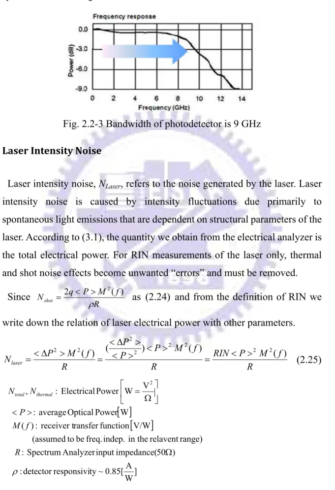
Fig. 2.2-3 Bandwidth of photodetector is 9 GHz ... 14

Fig. 2.2-4 The spectrum analyzer applies a narrowband filter to the signal with a passband F (



). ... 16

Fig. 2.2-5 the measurement of the system noise would be very similar to the thermal noise ... 18

Fig. 2.2-6 the noise of the laser far exceeds the shot or thermal noise terms 18 Fig. 3.2-2 Light-current relation ... 20

Fig. 3.2-2 Laser spectra from 10-30 ℃ ... 20

Fig. 3.3-1 RIN Level of -155 dB/Hz ... 21

Fig. 3.4-1 RIN spectra of DFB at 20℃ ... 22

Fig. 3.4-2 RIN spectra of DFB laser at 20℃ with the corresponding fit. The dark solid lines were fitting lines. ... 23

Fig. 3.4-3 D coefficient deriving from the plot of fr versus square root of the optical power ... 24

Fig. 3.4-4 The D coefficient was found from the slope of the fr versus P1/2. . 25

Fig. 3.4-5 fr were replotted as a function of the (I-Ith)1/2 ... 25

Fig. 3.5-1 (a)-(d) RIN spectra at three temperatures: 10 ,℃ 20 ℃, 30 ℃, and 40 ℃ ... 26

Fig. 3.5-2 Fixing the bias current at 12 mA, the fR at 10 ℃ is about 3 GHz higher than that at 40 ℃ while the RIN spectrum is more flattened at

(12)

10 ℃. ... 27

Fig. 3.5-3 fR versus (I-Ith)1/2 at four ambient temperatures. ... 28

Fig. 3.5-4 Differential gains against temperature showed strong temperature dependence. ... 29

Fig. 3.5-5 The K-factor is plotted as a function of temperature, which is insensitive to temperature. ... 29

Fig. 4.1-1 The schematic diagram of chirped multilayer QD structure. ... 31

Fig. 4.2-1 CW L-I curve measured at 20 ℃ ... 32

Fig. 4.2-3 Model gain-current relation in [13] ... 33

Fig. 4.2-2 Laser spectra for three cavity lengths at 20℃. ... 33

Fig. 4.3-1 Schematic diagram of QD laser structure and RIN spectrum ... 35

Fig. 4.3-2 RIN spectra for different laser power levels in 2007 ... 35

Fig. 4.3-3 (a)-(d) Evolution of measured noise spectral density with increasing bias current ... 36

Fig. 4.4-1 RIN spectra and corresponding solid fitted lines of 750 m ... 39

Fig. 4.4-2 K-factor of CMQD Laser with L =750 m ... 39

Fig. 4.5-1 (a)-(c) RIN spectra with different cavity lengths ... 41

Fig. 4.5-2 For three lasers with different L of 750 m, 1000 m, and 1500 m, the fR verse (I-Ith)1/2 were shown together ... 43

Fig. 4.6-1 double resonance frequencies RIN spectra were observed in even shorter cavity ... 46

(13)

Chapter 1 Introduction

Intensity Noise refers to power fluctuations in the lightwave signal. When the power fluctuations normalized to its average value, we call it relative intensity noise (RIN). According to the laser dynamics, the laser RIN spectra carry out two pieces of important information: maximum noise amplitude and maximum modulation bandwidth of the light sources.

Laser intensity noise is one of the limiting factors in the transmission of analog or digital signals, since intensity noise reduces signal-to-noise ratios (S/N) so that increases bit error rates. The noise level is necessary to be defined so that the noise amplitude can be quantified. In addition, it needs to modulate information onto light sources. To meet the quest for faster information transfer rates, RIN provides a method to estimate maximum modulation bandwidth of the lasers. In brief, RIN serves as a quality indicator of laser devices.

Compared with direct modulation response of lasers, RIN measurement reveals the intrinsic information of damping rate, and modulation bandwidth without any electrical parasitics. Moreover, RIN measurement can be done by direct probe test without additional package cost and time.

RIN of quantum well lasers are well studied in the literature. However, little work has been performed so far on quantum dot lasers owing to some limitation. In this thesis, we demonstrate the dynamic behavior of multiple Quantum well DFB laser and characterize that of Chirped Multilayer Quantum Dot Lasers.

(14)

Chapter 2 Theoretical Fundamentals and

Experimental Techniques

2.1 Theoretical Fundamentals

2.1.1 Characteristics of Quantum Dot Lasers

Density of state

Electron confinement within sufficiently narrow region of semiconductor material can significant change the energy spectrum. Size-quantization also has noticeable effects on the density of state (DOS) of the active region. Thus, the family of possible dimensionalities of the laser-active region involves bulky semiconductor epilayer (three-dimensional), thin epitaxial layer of quantum well (two-dimensional), elongated tube of quantum wire (one-dimensional) and self-assemble quantum dot (zero-dimensionl). All these four cases are shown schematically in Fig. 2.2-1

In the ultimate case of QD, the only allowed energy states correspond to discrete quantum levels of the QD. Density of states represents a set of delta-function peaks centered at the atomic-like energy levels. There are two main advantages of delta-function like DOS in QD lasers: low transparency carrier density result in low threshold current density and temperature stable operation; Low linewidth enhancement factor leads high-speed modulation. However, the dot size of self-assembled QDs growth by Stranski-Krastanov (S-K) growth mode is not ideally uniform. Size fluctuation of QDs gives rise inhomogeneous broadening about 30-50 meV. Moreover, single energy level also broaden homogeneously about 5-10 meV due to uncertainty principles.

(15)

Therefore, the DOS of QDs laser is Gaussian-like distribution rather than delta-like in ideal case.

Fig. 2.1-1 Density of States of Various Quantum Structure

Gaincurrent relation [1]

In addition to the ground state (GS) level, one or more excited-state (ES) levels can be thermally populated. In addition, these excited levels have higher degeneracy and, consequently, the higher saturated gain. Thus, the transition of the lasing line from the GS to the ES can be observed with increasing loss. m i th g gmod   







(2.1)

This situation is schematically presented in Fig. 2.1-2, where the gain-current dependence is schematically shown for the ground level of the ideal QD array as well as two subbands (ground and first excited) of a self-organized array. Due to non-ideality of the self-organized array discussed above, their gain-current characteristic demonstrates higher transparency current density, lower saturation gain, and less abrupt increase of the gain on

(16)

increasing the current density. g-J curve, which corresponds to the excited subband, is characterized by the higher saturated gain and higher transparency current density as compared to those of the ground subbands owing to a large concentration of available states on the excited level.

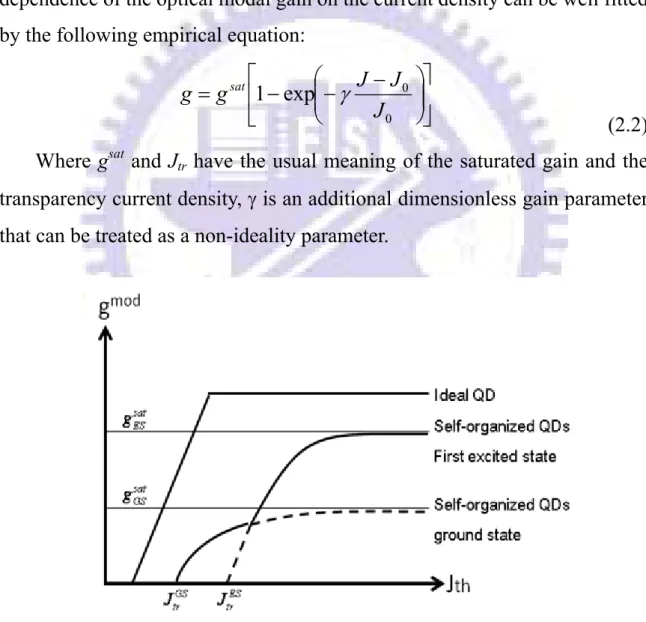
Taking into account the existence of higher-energy states, inhomogeneous broadening and possible non-equilibrium carrier distribution, complete theoretical description of the gain characteristics of QD lasers is a complicated problem. Zhukov et al. [2] has proposed in 1999 that the experimental dependence of the optical modal gain on the current density can be well fitted by the following empirical equation:

           _    0 0 exp 1 J J J g g sat

_

(2.2)

Where gsat and Jtr have the usual meaning of the saturated gain and the transparency current density,  is an additional dimensionless gain parameter that can be treated as a non-ideality parameter.

Fig. 2.1-2 Schematic dependence of the optical gain on the current density for the ideal and real (self-organized) QDs.

(17)

2.1.2 Theory of RIN Spectra

Definition of RIN

Relative Intensity Noise was measured under continuous-wave (CW) condition. RIN can be thought of as a type of inverse carrier-to-noise-ratio measurement. RIN is defined to be the ratio of the mean-square optical intensity noise to the square of the average optical power:

Hz dB/ 2 2 P P RIN    (2.3) where  2

P is the mean-square optical intensity fluctuation (in a 1-Hz

bandwidth) at specified frequency, and P is the average optical power. Singlemode RIN [3]

An expression for the RIN may be derived from the single-mode (strictly for single-longitudinal mode) rate equations for the photon and carrier density which may be written as:

 

F

 

t V R s s n g dt dS s sp ph g                 , 1 (2.4) l

 

n s s F

 

t g n qV I dt dn n g e      ,  (2.5)

where S, n are the photon and carrier densities in the active region, Fs(t) and Fn(t) are the Langevin noise terms, g(n, s) is the electronic gain, Rsp is the

spontaneous emission rate into the lasing mode, I is the injection current, V is the volume of the active region,  is the confinement factor, τe and τph are the electron and photon decay times, and υg is the group velocity. By using the standard small signal analysis with the use of the diffusion relations for the noise terms[4] , the RIN is found to be:

(18)

2 2 2 2 2 2 2 ) ( ) 1 ( 2 1 1 2                               _                r sp g n e sp sp g n sp dn dR V s a s R n dn dR V s a sV R RIN (2.6)

Where the resonant frequency



R and the damping



are given by ) )( 1 ( 2 _g _g _s dn dR V s a sp _g _g _s g n s r           (2.7) n s









(2.8)

And the parameter Γs and Γn are defined by: s g sV R s g sp s     (2.9)          e s g n n dn d s g   (2.10) a = dg(n, s)/dn is the differential gain and gs = dg(n,s)/ds is the nonlinear gain. To a good approximation, a single term dominates (2.7), hence the resonant frequency and damping may be written

2 / 1 2 / 1 ₍ _/ ₎ ) ( _g _g _g _ph r



a s



a



a s





     (2.11)             e ph r s g sp n dn d s g sV R      2 (2.12) The first term of (2.12) is small except at very low output powers. It is convenient to introduce the parameters D and K such that

f r D P f   (2.13) ' / 1 2 _   Kf_R  (2.14)

Where fR = (



o / 2n), Pf is the output power per facet and the term 1/ τ‘ corresponds to the last term of (2.12). D and K act as figures of merit

characterizing the frequency response of the laser, such that high-speed performance is expected from devices with a high value of D and low value of K. From (2.11) and (2.12):

(19)

2 / 1 int ₁ 2 _                m g h a V D     (2.15)

 



g a



K  2 2_ph 1 _s/ (2.16)

Where αint and αm are the internal and mirror losses, respectively. To take into account the nonlinear gain, the electronic gain is commonly approximated by:

 

n s g

 

n s



g ,  ₀ 1

(2.17)

Where  is the nonlinear gain coefficient. Then, using the condition for threshold, the damping coefficient may be written as:

 



a



K  2 2_ph/_g

(2.18)

According to (2.6), the measured RIN spectra were fitted to the following form, using four parameters:



2 2



2 2 2













r

B

A

RIN

(2.19) It was found that all the RIN spectra could be well fitted to this form, with the second term of the numerator dominant for frequencies above 2 GHz, and that the parameters



R and



could be accurately determined. In addition, in almost all the devices measured, it was found that the resonant frequency and damping were extremely well described by (2.13) and (2.14) up to powers of ~10 mW.

According to rate-equation analysis, resonance frequency and damping factor are the same in intrinsic frequency response and in intensity noise. Since the noise is internally generated and is not filtered through the parasitic elements, noise measurements give the true intrinsic peak frequency and the true damping factor.

The knowledge of fR and



allows the estimation of several figures of merit giving indications about the laser’s intrinsic dynamic behavior, the most

(20)

important being the well-known K factor [5]. The K factor, given in nanoseconds, is the slope of the  versus fR2 and is related to the maximum achievable intrinsic 3 dB small signal modulation frequency through (2.20)

K f_max  2 2

(2.20) The relaxation oscillation frequency can be described as follows:

2 p p g r aN     (2.21) Where τp is photon density, a is differential gain, group velocity, photon lifetime. Therefore, the differential gain can be calculated via (2.13) and (2.14).

The actual laser performance account for the parasitic and it only reach power levels way above the usual operating domain. Therefore, another figure of merit must be considered together with the K factor before to draw any conclusion about the device’s modulation capability.

Ideally, a device should combine a low K factor and a high D factor, meaning that a high modulation bandwidth can be reached at moderate optical power levels.

Multimode RIN

The equivalent equations for multimode operation may be obtained by taking the sums of the above equations for each mode, with photon density si,

ai (n, si,…,sm) and noise term Fs,i(t). However, except at low frequencies (below the frequencies of interest in this thesis) the single-mode equations provide a sufficiently good description [6]for multimode lasers provided all modes are included in the received power. On the other hand, if only one mode is filtered out from a multimode spectrum, it is typically found to contain a much larger noise level, especially at the low frequency. This is because of

(21)

mode partitioning. The energy tends to switch back and forth randomly between the various modes observed in the time-averaged spectrum causing larger power fluctuations in any one mode. If all modes are included, the net power tends to average out these fluctuations.

(22)

2.2 Experimental Techniques

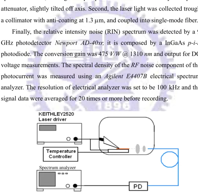
2.2.1 Measurement Setup

The schematic diagram for the measurement of RIN spectra is shown in Fig. 2.2-1. As-cleaved lasers were placed on a temperature controlled copper stage. KEITHLEY 2520 is the laser driver to injecte current. To lower the optical feedback, the light output power was first reduced by an optical attenuator, slightly tilted off axis. Second, the laser light was collected trough a collimator with anti-coating at 1.3 m, and coupled into single-mode fiber.

Finally, the relative intensity noise (RIN) spectrum was detected by a 9 GHz photodetector Newport AD-40xr, it is composed by a InGaAs p-i-n photodiode. The conversion gain was 475 V/W @ 1310 nm and output for DC voltage measurements. The spectral density of the RF noise component of the photocurrent was measured using an Agilent E4407B electrical spectrum analyzer. The resolution of electrical analyzer was set to be 100 kHz and the signal data were averaged for 20 times or more before recording.

(23)

2.2.2 Corrected Laser Intensity noise

The noise at the receiver output results from three fundamental contributions: laser intensity noise, thermal noise and shot noise. The total system noise, NT(f), is the summation of these three noise sources.

NT (f) = NLaser(f) + Nshot + Nthermal(f) [W/Hz] (2.22) where: NLaser(f) is the laser intensity noise power per Hz;

Nshot is the photonic shot noise power per Hz;

Nthermal(f) is the contribution of thermal noise power per Hz; While it is desirable to determine the laser noise, it is also valuable to determine separately the individual contributions of shot and thermal noise.

Thermal Noise

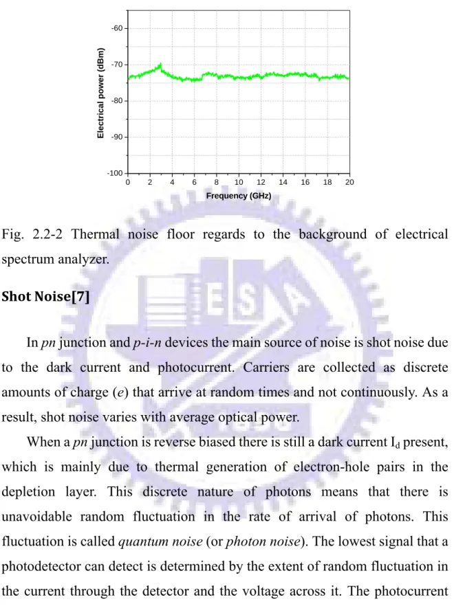
The amplifier and electronics that follow the photodiode produce thermal noise. Thermal noise is input power independent, which is the electronic noise, generated by the thermal agitation of the charge carriers inside a conductor at equilibrium and regardless of any applied voltage. Therefore, we refer the background value of the Electrum Analyzer to the thermal noise. The thermal background of our Electrum Analyzer is shown in Fig. 2.2-2.

We express thermal noise in dB relative to the room temperature and the lower limit of –174 dBm/Hz. Electrical spectrum analyzers usually have noise figures of 30 dB or higher. For a system at a given temperature, thermal noise is usually constant for every frequency component.

(24)

0 2 4 6 8 10 12 14 16 18 20 -100 -90 -80 -70 -60 E lec tr ical pow er ( d Bm ) Frequency (GHz)

Fig. 2.2-2 Thermal noise floor regards to the background of electrical spectrum analyzer.

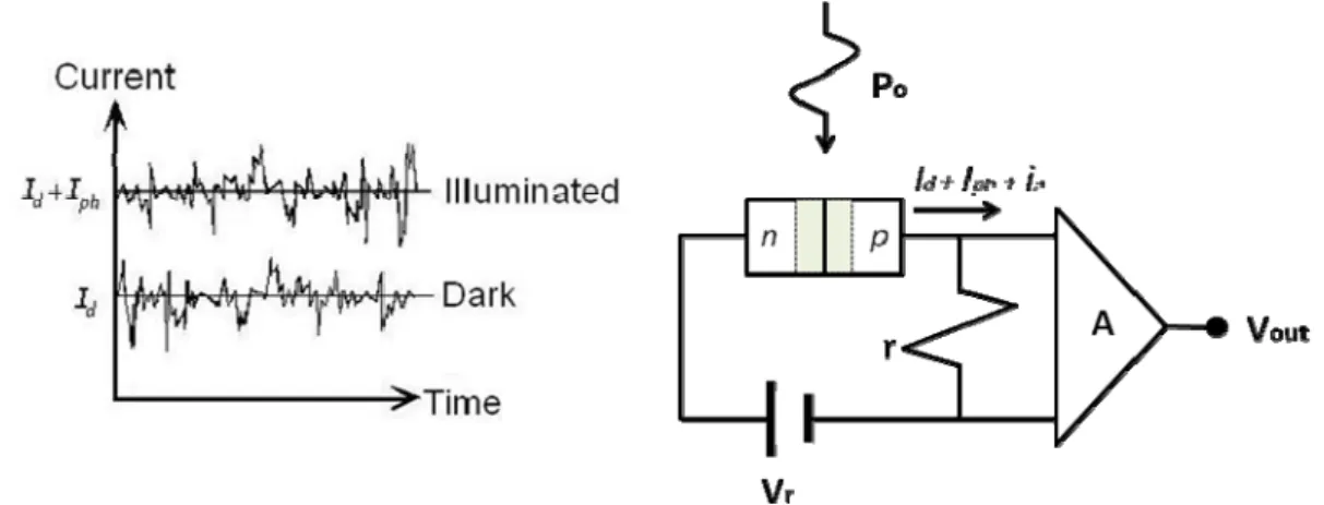
Shot Noise[7]

In pn junction and p-i-n devices the main source of noise is shot noise due to the dark current and photocurrent. Carriers are collected as discrete amounts of charge (e) that arrive at random times and not continuously. As a result, shot noise varies with average optical power.

When a pn junction is reverse biased there is still a dark current Id present,

which is mainly due to thermal generation of electron-hole pairs in the depletion layer. This discrete nature of photons means that there is unavoidable random fluctuation in the rate of arrival of photons. This fluctuation is called quantum noise (or photon noise). The lowest signal that a photodetector can detect is determined by the extent of random fluctuation in the current through the detector and the voltage across it. The photocurrent signal must be greater than the shot noise in the dark current.

(25)

Fig. 2.2-2 In pn junction and pin devices the main source of noise is shot noise due to the dark current and photocurrent.

We have photon current Iph out of the photodiode due to the average optical power input, the noise produced is related directly to the amount of light incident on the photodetector. The shot noise, generated in the photo detector, has a white Gaussian statistical distribution and an root-mean-square (RMS) spectral density:

<i2>shot =2qIph=2q



<P> (2.23) Where q is the elementary electron charge (1.60  10–19_{coulomb), }

_

_{is the}

detector responsivity which takes on the value of 0.85 ± 0.05 A/W and is assumed to be frequency independent in the relevant range of 0 to 9 Hz (Fig. 2.2-3) and < P > is the average optical power at the receiver input.

For the amplified photodetector, the transfer function, M (f ), is 475 V/W at 1310 nm. From the familiar equation P=V2/R where the input impedance (R) of the Spectrum analyzer is 50 , the optical power converted to electrical output power. Therefore, the shot-noise power, Nshot becomes:

) ( 2 2 R f M P q N_shot     (2.24) In addition, great care must be taken when using this subtraction method to determine the laser RIN. In subtracting small numbers from small numbers, errors in values that are close to the excess-noise value of the laser can have

(26)

large effects. It is important to know the frequency response for the total system before making noise subtractions.

Fig. 2.2-3 Bandwidth of photodetector is 9 GHz

Laser Intensity Noise

Laser intensity noise, NLaser, refers to the noise generated by the laser. Laser intensity noise is caused by intensity fluctuations due primarily to spontaneous light emissions that are dependent on structural parameters of the laser. According to (3.1), the quantity we obtain from the electrical analyzer is the total electrical power. For RIN measurements of the laser only, thermal and shot noise effects become unwanted “errors” and must be removed.

Since 2 ( ) 2 R f M P q N_shot   

 as (2.24) and from the definition of RIN we write down the relation of laser electrical power with other parameters.

R f M P RIN R f M P P P R f M P N_laser ( ) ) ( ) ( ) ( ₂ 2 2 2 2 2 2 2 _ _              (2.25)

 





A ) 50 impedance( input Analyzer Spectrum : range) relavent in the indep. freq. be to (assumed V/W function ransfer receiver t : ) ( W Power Optical average : V W Power Electrical : , 2             R f M P N N_total _thermal

(27)

 

dB , ) ( ) ( 2 ) ( log 10 ₂ ₂ 2                       P f M P f qM N N R RIN thermal total

_

(2.26) Resolution Bandwidth [8]

We use a spectrum analyzer to measure the electrical power (the square of the optical power) associated with the noise. We assume that the spectrum analyzer applies a narrowband filter to the signal with a passband described by F (



), then the measured mean-square time-averaged signal would be given by:

 

         ( ) ( ')* ( ) ( ')* ' ) 2 ( 1 ) ( ( )' 2 2 _ _ _ _ _ _ _ _  _P _t _P _P _F _F _ej  t_d _d (2.27) For completely random noise, the magnitude of the noise at any given frequency is completely uncorrelated with the magnitude of the noise at any other frequency. As a result, when the product of the two frequency component is averaged over time is a delta function. The strength of the delta function correlation is defined as the spectral density,SP(), of P()at  :

) ' ( 2 ) ( )* ' ( ) (













 _    P P S _P (2.28)

We say that the measurement filter is centered at 0, and is narrowband

relative to variations in the spectral density, then withF()1 we obtain

f

S

df

F

S

t

P



_P



_P









  

(

)

(

)

2 )

(

)

(

2 ₀ 0 2

_



_ _ (2.29)

Note that 2f is regarded as both positive and negative frequency. If the spectral density is defined as single-sided, then the factor 2 should be removed.

The measurement bandwidth can vary from application to application, it is common to specify the quantity in dB/Hz or Relative Intensity Noise per

(28)

unit bandwidth. The full intensity noise is found by integrating the RIN per unit bandwidth over the detection bandwidth of the system of practical interest. Therefore, the required RIN per unit bandwidth of the laser is found from:

]) [ ( log 10 ) ( ) / (dB Hz RIN dB ₁₀ f Hz RIN    (2.30)

Consequently, if the system bandwidth is increased, the laser RIN per unit bandwidth must be decreased in order to maintain the same total RIN.

Fig. 2.2-4 The spectrum analyzer applies a narrowband filter to the signal with a passband F (



).

Finally, consider the entire factor influence absolute laser RIN, this chapter has given an efficacious calibration formula as follows:

                            Hz dB , ) ( ) ( 2 ) ( log 10 ₂ ₂ 2 f P f M P f qM N N R f

RIN total thermal



(2.31)

 

Hz bandwidth Resolution : where f

(29)

2.2.3 Limitation

The noise at the receiver output results from three fundamental contributions: laser intensity noise primarily due to spontaneous light emissions; thermal noise from the electronics; and photonic shot noise.

To evaluate laser-intensity noise contributions in this chapter, the relative-intensity-noise specification, RIN, was developed. This measurement is the ratio of the laser intensity noise to the average power of the laser, in equivalent electrical units. Work on improving laser intensity noise continues. In some cases, the intensity noise levels of the laser can approach the noise limitations of measurement system. There are some limits to measuring the noise contribution of the laser we should be notified for measuring the laser Intensity noise.

In Fig. 2.2-5 [9]the measurement of the system noise would be very similar to the thermal noise, thus an accurate measurement of the laser noise is difficult to achieve. A large amount of averaging could be employed; however, only the RIN peak would be observed, rather than the full RIN spectrum. When the noise of the laser far exceeds the shot or thermal noise terms, the total system noise is essentially equal to the laser intensity noise as shown in Fig. 2.2-6. In such cases, RIN Laser equals RIN System. However, as laser quality improves and the intensity-noise level decreases, the effects of shot and thermal-noise sources become more significant in RIN measurements.

(30)

Fig. 2.2-5 the measurement of the system noise would be very similar to the thermal noise

(31)

Chapter 3 Multiple Quantum Well DFB Laser

3.1 Device Specification

We demonstrated RIN characteristics of a commercial MQW DFB laser. The attached specification is shown in Table. 3.1-1. The DFB laser package in a 14 pin ‘butterfly’ type module. The module couples the laser output through a optical isolator in-line into a single mode fiber. The module also includes a monitor photodiode, a thermoelectric cooler (TEC) and a thermistor.

(32)

3.2 Static characteristics

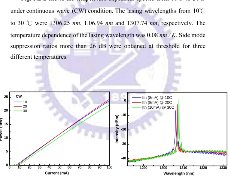
Temperature dependence of the light output versus the current characteristics is shown in Fig. 3.2-1. The measurement was done under a CW operation from 10 ℃ to 30 ℃ The threshold current at 20 ℃ was 7.5 mA. Good linearity maintained up to a bias current of 10 times the threshold with the slope efficiency of 25.5 %.

Fig. 3.2-2 shows the temperature dependent spectra from 10℃ to 30℃ under continuous wave (CW) condition. The lasing wavelengths from 10℃ to 30 ℃ were 1306.25 nm, 1.06.94 nm and 1307.74 nm, respectively. The temperature dependence of the lasing wavelength was 0.08 nm / K. Side mode suppression ratios more than 26 dB were obtained at threshold for three different temperatures. 0 10 20 30 40 50 60 70 80 90 100 0 5 10 15 20 25 10 20 30 Current (mA) Po we r (m W ) CW 1290 1300 1310 1320 1330 -40 -30 -20 -10 0 Inten s it y ( d B m ) Ith (8mA) @ 10C Ith (8mA) @ 20C Ith (10mA) @ 30C Wavelength (nm)

(33)

3.3 RIN level

The measured RIN spectrums for DFB laser operated under 60 mA and taken at 20 are℃ plotted in Fig. 3.3-1. To obtain a correct RIN level, each measured electrical noise spectral density function has to be corrected for the thermal and shot noise contributions. By the calibration formula derived in chapter 2, we obtained RIN level of –155 dB/Hz.

Calibrated RIN level is consistent with the laser specification; the accuracy of the measurement is therefore confirmed. This level is also comparable to that of conventional well-designed DFB lasers.

2 4 6 8 10 12 14 16 18 20 22 24 -175 -170 -165 -160 -155 -150 -145 -140 -135 -130 -125

Operate w/ 60mA @ 20OC 60mA

RI

N (d

B/

Hz)

Frequency (GHz)

(34)

3.4 Modulation bandwidth and Differential gain

Using our experimental setup, we followed noise variations up to 12 GHz. The measured RIN spectra for DFB laser with different injection currents taken at 20 ℃ are plotted in Fig. 3.4-1. Under CW bias conditions, as the current increases, the peak frequency (resonance frequency) shifted to a higher frequency. At low frequencies, the RIN level increased due to the detection system. The periodic response at high frequencies was stemmed from an electronic oscillatory response of the amplifier [10].

1 2 3 4 5 6 7 8 9 10 11 12 -170 -160 -150 -140 -130 -120 -110 -100 _8mA 9mA 10mA 12mA 14mA 16mA RIN (d B /Hz) Frequency (GHz)

Fig. 3.4-1 RIN spectra of DFB at 20℃

Fig. 3-4-2 depicts measured data with the corresponding fit. The curves were well fitted to Eq. (2.19). The fitted fR and



are listed in Tafble 3-4-1. Both parameters increased with increasing operating current.A typical plot of

(35)

a slope of 0.326 ns (K-factor), which indicates a 3 dB modulation bandwidth in excess of 27 GHz by Eq. (2.20).

Fig. 3.4-2 RIN spectra of DFB laser at 20℃ with the corresponding fit. The dark solid lines were fitting lines.

Table 3.4-1 Fitted fR and



of DFB laser at 20 ℃. Operating Current fR (GHz)

ԃ

(s-1) 1.1 Ith 1.27 3.49109 1.2 Ith 2.50 4.81109 1.3 Ith 3.27 6.54109 1.6 Ith 4.46 9.14109 1.9 Ith 5.41 1.281010 2.1 Ith 6.45 1.631010 2μ 109 _{4μ 10}9 _{6μ 10}9 ₈_{μ 10}9 FrequencyHz RIN 1 Hz 

(36)

-10 0 10 20 30 40 50 0 5 10 15 20 D a mp ing ( 10 9 s ) (Resonance Frequency)2(GHz)2 K=0.326ns

Fig. 3.4-3. K-factor derived from the slope of damping factor (



) verse square of resonance frequency (fr2).

The D coefficient was found to be 4.11 GHz/mW1/2 from the slope of the fr versus square root of the optical power curve, as illustrated in Fig. 3.4-4 .The good linearity of the curve also assesses the validity of both the model and the measurement.

For the mode spacing of 0.75 nm at 20 ℃ as in Fig. 3.2-2, the cavity length and refractive index are estimated to be 300 m and 3.8. We further assume the optical mode volume to be 300 m1.5 m 0.4 m ( L



w



d ). Both Internal quantum efficiency and couple efficiency for the single-mode fiber pigtail package are taken to be 80 %. The quantum efficiency is measured to be 25.5 % as mentioned in the previous section. Therefore, the differential gain is estimated to be. In Fig. 3.4-5, the data in Fig. 3.4-4 were replotted as a function of the ₆_₁₀16_cm2_{square root of current (I-I}

th), where I is the bias current, Ith is the threshold current. Since P0  (I  Ith), the

(37)

multiplied by the square root of



(0.268 mW/mA at 20℃). 0.0 0.2 0.4 0.6 0.8 1.0 1.2 1.4 1.6 0 1 2 3 4 5 6 7 8 D=4.11 GHz/mW1/2 R e sonance Fr equ e ncy ( G H z ) Power1/2(mW1/2)

Fig. 3.4-4 The D coefficient was found from the slope of the fr versus P1/2.

0.0 0.5 1.0 1.5 2.0 2.5 3.0 3.5 0 1 2 3 4 5 6 7 8 R esonance Frequency (G H z ) (_I-Ith)1/2(mA) 2.13GHz/mA1/2

(38)

3.5 Temperature Characteristics of MQW lasers

Fig. 3.5-1(a)–(d) show the RIN spectra at three temperatures: 10 ℃, 20 ℃, 30 ℃, and 40 ℃. The relaxation peaks move toward high frequency as the DC bias increased.Nevertheless, if we fix the bias current at a value of 12 mA as Fig 4.5-2 demonstrated, the resonance frequency at 10 ℃ is about 3 GHz higher than that at 40 ℃ while the RIN spectrum is more flattened at 10℃. The above observations are interpreted as follows.

1 2 3 4 5 6 7 8 9 10 11 12 -170 -160 -150 -140 -130 -120 -110 -100 (a) 10 oC 8mA 9mA 10mA 12mA 14mA 16mA RIN (dB/Hz) Frequency (GHz) 1 2 3 4 5 6 7 8 9 10 11 12 -170 -160 -150 -140 -130 -120 -110 -100 (b) 20OC 8mA 9mA 10mA 12mA 14mA 16mA RIN ( d B/Hz) Frequency (GHz) 1 2 3 4 5 6 7 8 9 10 11 12 -170 -160 -150 -140 -130 -120 -110 -100 (c) 30OC 10mA 12mA 14mA 16mA RIN (d B/H z ) Frequency (GHz) 1 2 3 4 5 6 7 8 -170 -160 -150 -140 -130 -120 -110 -100 (d) 40 oC 12mA 13mA 15mA 17mA RIN (d B/Hz) Frequency (GHz)

(39)

1 2 3 4 5 6 7 8 -170 -160 -150 -140 -130 -120 -110 -100 40OC 30OC 20OC 10OC R IN (dB/ H z ) Frequency (GHz) 12mA

Fig. 3.5-2 Fixing the bias current at 12 mA, the fR at 10 ℃ is about 3 GHz higher than that at 40 ℃ while the RIN spectrum is more flattened at 10 ℃.

The fitting procedure described above is applied to of the measured RIN spectrum. Fig. 3.5-3 shows the relaxation oscillation frequency versus square root of current at four ambient temperatures. The proportional factor D is found to vary from 1.8 GH/mA1/2 at 40 ℃ to 2.3 GH/mA1/2 at 10 ℃. Therefore, the differential gain shows strong temperature dependence and is plotted in Fig. 3.5-4 over the temperature range plotted, the differential gain decreases by a factor of approximately 1.5, which shows a linear function of the temperature [11]. Increasing temperature can result in altered gain characteristics. Besides the broadening of the Fermi occupation, probability function spreads the carriers over a larger energy range for a given overall carrier density. It is to say that a lower spectral concentration of inverted carriers leads to a broadening and flattening of the gain spectrum. Furthermore, thermionic emission of electrons from the QW to the barrier region enhanced at high temperatures. These effects contribute to strong recombination outside the QW and carrier leakage. Since the increased carrier population in the barrier region does not contribute to the optical gain, the differential gain

(40)

decreases rapidly at high temperatures. Consequently, the smaller differential gain at 40 ℃ leads to lower resonance frequency as Eq. (2.21) stated.

In addition, RIN spectrum is flatten at higher resonance frequency because of larger damping factor. We can understand it from the linear relationship between damping term and square of resonance frequency. The carrier transport effect increases with increasing band discontinuities and barrier width, which determines the modulation bandwidth for QW lasers. The nature of K-factor reported in the literature was that the more number of wells the less sensitive to temperature [12]. For single-QW lasers, the K-factor can vary by two times for 200 to 350 k. Since the K- factor in Fig. 3.4-5 is independent on temperature, we conclude that this commercial DFB contains more than eight layers of QW in the active region.

0.0 0.5 1.0 1.5 2.0 2.5 3.0 3.5 0 1 2 3 4 5 6 7 8 Reso nance Freq uency ( G Hz) (_I-Ith)1/2(mA) Temp. ---10OC 2.24 GHz/vmA 20OC 2.13 GHz/vmA 30OC 2.00 GHz/vmA 40OC 1.79 GHz/vmA

(41)

10 15 20 25 30 35 40 1.1 1.2 1.3 1.4 1.5 1.6 1.7 Temperature (oC) D if fe re nt ia l ga in ( 10 -15 cm 2 )

Fig. 3.5-4 Differential gains against temperature showed strong temperature dependence. 0 5 10 15 20 25 30 35 40 45 50 0.0 0.1 0.2 0.3 0.4 0.5 0.6 Temperature (oC) K -fac to r ( ns )

Fig. 3.5-5 The K-factor is plotted as a function of temperature, which is insensitive to temperature.

(42)

3.6 Summary

The measured RIN level of the commercial DFB laser strongly confirmed the accuracy of the measurement and calibration.From the derived D coefficient and K-factor from the fitting procedure of room temperature RIN spectra, the calculated differential gain and modulation bandwidth are comparable to that of well-designed DFB lasers.

The temperature dependent measurement of RIN was demonstrated. From the tendency of D and K-factor, we observed the expected characteristics of multiple Quantum Well laser as the literature. The important characteristics are differential gain decrease linearly with temperature and K-factor is not sensitive to the temperature.

(43)

Chapter 4 Chirped Multilayer Quantum Dot

Laser

4.1 Device Structure

The chirped 10-layer QD laser was grown by molecular beam epitaxy (MBE). As the schematic diagram shown in Fig. 4.1-1, chirped multilayer QD (CMQD) lasers with 2-, 3- and 5-layer of long-, medium- and short-wavelength QD stacks (designated as 2*QDL, 3*QDM and 5*QDs) were

engineered in the laser structure, which correspond to InAs QDs of 2.6 ML capped by InGaAs of 4 nm, 3 nm and 1 nm, respectively. The staking sequence was arranged so that QDL was near the n-side. Fabrication details

can be found in our previous work in [13].

Various cavity lengths of 750 m, 1000 m, and 1500 m were then analyzed by RIN characteristics. CMQD lasers contain many layers in the active region so that slower carrier dynamics discussed in MQW DFB laser may play an important role.

(44)

4.2 Static Characteristics

Fig. 4.2-1 shows a CW L-I curves measured at 20 . The slope ℃ efficiency of 0.59 %, 0.49 %, and 0.50 % for cavity length (L) of 750 m, 1000 m, and 1500 m, respectively, up to a bias of ~100 mA. Fig. 4.2-2 is a plot of the laser emission spectra with cavity lengths with 750 m, 1000 m, and 1500 m. None of them emitting in single wavelength, several modes exist simultaneously. In addition, threshold current densities and the center wavelengths are shown in Table 4.2-1. The threshold current densities range from 453.3 A/cm2 to 888.8 A/cm2 corresponding to QDL excited state lasing

which confirmed by modal gain analysis in Fig. 4.2-3as our previous work presented [13]. The QDL excited state (ES) and QDM ground state (GS) were

suppose to be 1183 nm and 1230 nm, however center wavelengths of three QDL ES lasing devices were red shift to the range of 1195 nm to 1212 nm.

This is because the small energy difference between QDM GS and QDL ES

such that carriers from QDM GS contribute to the tail of QDL ES gain profile.

0 20 40 60 80 100 120 0 5 10 15 20 25 30 35 40 m _d=0.59% m_d=0.49% m _d=0.50% T o w facet P o wer (mW) W: 5um 20oC Current (mA)

(45)

Fig. 4.2-3 Model gain-current relation in [13]

Table 4.2-1 Center λ and threshold current densities of three cavity lengths

L (mm) 0.75 1.0 1.5 λ (nm) @ Ith 1198 1204 1212 Jth (A/cm 2 ) 888.8 660.0 453.3 1195 1200 1205 1210 -40 -30 -20 -10 0 Wavelength (nm) 1.3 Ith (40mA) -30 -20 -10 0 (L,W)=(1.0mm,5um) 2.2 Ith (70mA) 1195 1200 1205 -40 -30 -20 -10 0 Intens it y (dBm) 1.2Ith (40mA) -40 -30 -20 -10 0 10 (L,W)=(0.75mm,5um) 1.8 Ith (60mA) 1205 1210 1215 1220 -40 -30 -20 -10 0 1.2 Ith (40mA) -40 -30 -20 -10 0 (L,W)=(1.5mm,5um) 2.0 Ith (70mA)

(46)

4.3 RIN Level of Quantum Dot laser

In contrast to the QW lasers, the small signal modulation response in QD lasers is known to be highly damped [14,15] and the maximum modulation bandwidth is limited to below 10 – 12 GHz for lasers operating in the long wavelength of 1300-1500 nm [16-18].

The differential gain was shown to reduce due to the state filling effect as well as carrier capture process [19,20], which further limiting the high frequency modulation capabilities. The modulation characteristics and the noise spectra are governed by the same dynamic processes. The highly damped limited bandwidth modulation response of QD lasers therefore leads unique low noise characteristics. The very low RIN levels make QD lasers suitable light sources for use in analog transmission applications. However, it was more difficult to measure the weak noise signal of QD laser. Consequently, empirical noise spectra of QD laser can rarely be found in the publication.

In 2006, the measured relative intensity noise levels of multi-stack quantum dash laser operating at 1320 nm was first demonstrated as low as -160 dB/Hz as shown in Fig. 4.3-1 [21]. In 2007, the RIN spectrum with different DC bias levels of 15-layer QD laser was presented (Fig. 4.3-2). The RIN level was extract to be -158 ~ -160 dB/Hz at high optical powers. Nevertheless, the actual RIN is somewhat masked by the electrical resonances at high frequencies [22].

(47)

Fig. 4.3-1 Schematic diagram of QD laser structure and RIN spectrum [20]

Fig. 4.3-2 RIN spectra for different laser power levels in 2007 [21] In our recent work, the RIN measurements of QD lasers were carried out. The noise power of QD lasers was in the order of Pico-watt, the slight difference of every spectral density recorded directly from the electrical spectrum analyzer has to be separated with attention. The vertical far-field angle is usually large for edged emitting laser structure. Moreover, the laser bar was titled a small angle off the optical axis to lower the optical feedback. Thus, it was more difficult to efficiently couple the optical power into a single-mode fiber (The couple efficiency of this sample was 12 %). Cares

(48)

must be taken while adjusting collimator for coupling, since the position with maximum focused optical power was extremely critical.

As-measured RIN spectra were shown, Fig 4.3-3 (a) – (d) depicts evolution of noise spectral density with increasing bias current, in which the electrical power of noise enlarged before 50 mA and then went down gradually. In addition, the sharp drop at 3 GHz was due to system error of spectrum analyzer.

In order to obtain correct RIN spectra, measured noise spectral density functions have to calibrate for the thermal and shot noise contribution as well. RIN spectra of our work shown in Fig. 4.3-3 (e) is clear presented in the order of rising bias current. The problem of electrical resonances was overcome with higher coupled power. It revealed that flat RIN spectra reached very low levels of -160 dB/ Hz, which is consistent with earlier observations.

1.5 2.0 2.5 3.0 3.5 4.0 0.2 0.4 0.6 0.8 1.0 1.2 (a) DO901 20O C L: 0.75mm W: 5um 40mA Frequency (GHz) El ec tri c al Po w e r ( pW ) 1.5 2.0 2.5 3.0 3.5 4.0 0.2 0.4 0.6 0.8 1.0 1.2 (b) DO901 20O C L: 0.75mm W: 5um 40mA 45mA 50mA Frequency (GHz) El ectri ca l Po w e r ( pW ) 1.5 2.0 2.5 3.0 3.5 4.0 0.2 0.4 0.6 0.8 1.0 1.2 (c) DO901 20O C L: 0.75mm W: 5um 55mA 60mA 70mA Frequency (GHz) El ectri cal Po w e r ( pW ) 1.5 2.0 2.5 3.0 3.5 4.0 0.2 0.4 0.6 0.8 1.0 1.2 (d) DO901 20OC L: 0.75mm W: 5um 40mA 45mA 50mA 55mA 60mA 70mA Frequency (GHz) El ectri ca l Po w e r ( pW )

(49)

0.5 1.0 1.5 2.0 2.5 3.0 3.5 4.0 4.5 -170 -160 -150 -140 -130 -120 (e) DO901 20OC L: 0.75mm W: 5um 40mA 45mA 50mA 55mA 60mA 70mA 80mA RI N ( d B /H z ) Frequency (GHz)

Fig. 4.3-3 (e) Calibrated RIN spectra reveals very low level as low as -160 dB/Hz

(50)

4.4 Excited State RIN spectra

As mentioned above, the modulation bandwidth of QD lasers is damping-limited due to the comparatively low saturated gain and slow carrier dynamics [23]. Fortunately, the situation could be somehow released if we can modulate excited state QD lasers. Modulation bandwidth of excited state is expected to be about two times of ground state. This is attributed to an increase in the saturated gain and reduced carrier scattering time of the excited state compared to the ground state. The direct modulation of excited state quantum dot lasers was first demonstrated experimentally by Stevens el al. in August 2009 [24]. In their study, the K-factor limited modulation bandwidth of ground state and excited state are 6.7 GHz and 13.0 GHz, respectively.

For our excited state lasing QD laser with cavity length of 750 m, the RIN spectrum was carried out as shown in the previous section and well-fitted with the Eq. (2.19) as in Fig. 4.4-1. The extracted K-factor was 0.628 ns in Fig. 4.4-2, and the predicted maximum modulation bandwidth of 14 GHz was comparable with Stevens’s work on excited state. On the other hand, we learned that the K-factor was insensitive to the temperature for the carrier dynamic limited devices. Therefore, the strong evidence certified again this is the RIN spectrum of excited state QD laser.

To the best of our knowledge, we have successfully demonstrated RIN spectrum of excited state QD for the first time.

(51)

Fig. 4.4-1 RIN spectra and corresponding solid fitted lines of 750 m 5.0 5.5 6.0 6.5 7.0 7.5 5.0 5.5 6.0 6.5 7.0 L=750um K=0.628ns (Resonance Frequency)2(GHz)2 D a m p ing ( 10 9 Ra d /s )

(52)

4.5 Different Cavity length

The QD laser RIN measurements were limited for short cavity lasers to avoid more modes lasing in the long cavity mode. Because of mode partitioning, the energy tends to switch back and forth randomly between the various modes observed in the time-averaged spectrum causing larger power fluctuations in any one mode. If all modes are included, the net power tends to average out these fluctuations. Fig 4.5-1 (a)-(c) show the RIN spectra for L of 750 m, 1000 m, and 1500 m, we could see that the spectra flatten out for 1500m. Thus, the RIN characteristic was even difficult to be observed in long cavity lasers. In general, cavity length for QD RIN measurement was suggested to be within 2 mm.

Now we comment on the profile of those RIN spectra with different cavity lengths. Compared to Fig. 4.4-1, the RIN spectra of 750 m shown in Fig. 4.5-1(a) were further biased to higher powers. To response the thermal effect in the previous section, we can see apparently the resonance frequencies for these higher power levels reduced along bended arrow line shown. In contrary, it was hard to see the resonance frequencies reducing in 1500 m in Fig. 4.5-1(c) by eyes and we considered the arrow line still went straightforward. This was because the lower current density of 1500 m somehow reduce junction heating. These observations confirmed our previous understanding of thermal effect.

(53)

0 .5 1 .0 1 .5 2 .0 2 .5 3 .0 3 .5 4 .0 4 .5 -1 7 0 -1 6 5 -1 6 0 -1 5 5 -1 5 0 -1 4 5 -1 4 0 -1 3 5 -1 3 0 -1 2 5 -1 2 0 L : 1 .0 m m W : 5 u m RIN (d B/Hz) 0 .5 1 .0 1 .5 2 .0 2 .5 3 .0 3 .5 4 .0 4 .5 -1 7 0 -1 6 5 -1 6 0 -1 5 5 -1 5 0 -1 4 5 -1 4 0 -1 3 5 -1 3 0 -1 2 5 -1 2 0 L : 0 .7 5 m m W : 5 u m RI N (d B /Hz) 0 .5 1 .0 1 .5 2 .0 2 .5 3 .0 3 .5 4 .0 4 .5 -1 7 0 -1 6 5 -1 6 0 -1 5 5 -1 5 0 -1 4 5 -1 4 0 -1 3 5 -1 3 0 -1 2 5 -1 2 0 L : 1 .5 m m W : 5 u m RI N ( d B/ H z ) F r e q u e n c y (G H z)

(54)

For three lasers with different cavity lengths ( 750 m, 1000 m, and 1500 m ), the resonance frequencies verse (I-Ith)1/2 were shown in Fig. 4.5-2 . One unexpected finding was observed: slope has a marked fall of linear fit and fitted line did not go through the zero. As a result, differential gain could not be obtained from the slope of fitting. By connecting each data point to the zero, we are confident that the differential gains should fall within the slopes individual, or we can say the resonance frequencies would be underestimated. The red dash lines for 750 m depict how resonance frequencies drop from the access line. The instantaneous differential gains were listed in Table 4.5-1, they declined from 8.210-16 _cm2_{to 3.010}-16_cm2_{. We learned that the}

differential gain as well as resonance frequency decrease linearly with increasing temperature in chapter 3. It is encouraging to turn the idea into this chapter. For our measuring, cleaved QD laser was barely placed on a temperature controlling heatsink. Compare to other packaged laser with a thermoelectric cooler included, temperature controlling of our QD laser was much less efficient. As a result, junction temperature rose rapidly and differential gain reduced with increasing power. In brief, differential gain fell due to heating effect. It was important information for RIN measurement of as-cleaved lasers.

(55)

0.0 1.0 2.0 3.0 4.0 5.0 6.0 0.0 1.0 2.0 3.0 4.0 Resonance f r (G Hz) L=750m 1000m 1500m Sqrt

(

_I-Ith

)

(

mA0.5

)

DO901 QD Lasers

W = 5



m

heating

Fig. 4.5-2 For three lasers with different L of 750 m, 1000 m, and 1500 m, the fR verse (I-Ith)1/2 were shown together

Table 4.5-1 Declining of the instantaneous differential gains

L=750 m_Ith=33.33mA Operating Current(mA) Current Density(A/cm2) a (cm 2₎ 40 (1.2Ith) 1067 8.210-16 45 (1.4Ith) 1200 5.410-16 50 (1.5Ith) 1333 4.010-16 55 (1.7Ith) 1467 3.410-16 60 (1.8Ith) 1600 3.010-16

(56)

At a fix value of (I-Ith)1/2 as black dash line illustrated, the differential gains, optical mode volumes and resonance frequencies could be compared in Table 4.5-2. Differential gain slightly decreased in short cavity length. That is because our threshold current density for 750 m most approached gain saturation that differential gain decreased base on the g-J relation of quantum dot lasers. In addition, optical mode volumes (Vp) also expand with cavity length. These two factors however lead opposite influences on the resonance as the following equation interpreted.





2 / 1

















_i _th p g R

I

qV

a







We could find the dominant factor determine the resonance frequency. Obviously, mode volume grew faster than differential gain result in a decline of resonance frequency in the longer cavity laser. Overall, for high-speed device a shorter cavity length may be optimum, moving the RIN peaks out to higher frequencies

Table 4.5-2 Parameters at a fix value of (I-Ith)1/2

L a (cm2) Vp (cm2) fR (GHz)

750



m 5.010-16 1.310-9 2.4

1000



m 5.410-16 1.810-9 2.2

(57)

4.6 Double Resonance Peaks

Finally, the most interesting finding of our work was that double resonance frequencies RIN spectra were observed in even shorter cavity of 600 m. As shown in Fig 4.6-1, it was somewhat surprising that the RIN spectra were well fitted if we added another term to the Eq. (2.19):

2 2 2 2 2 2 2 2 2 2 2 2 1 2 2 1 2 2 1 1 ) ( ) (











        r r B A B A RIN (4.1) The fitting parameters of peaks on the left were listed in Table 4.6-1. From the extracted K-factor of 0.68 ns, the maximum modulation bandwidth was extended to 13 GHz, which was considered excited state lasing. However, the second resonance frequencies kept fixed and we failed to define the K-factor.

In recent years, there has been some literature on multi-peak RIN spectra for VCSEL. There are two main suggestions for the cause of multi-peak RIN spectra. One believe that two-mode noise spectra incorporate the dependence on the degree of spatial overlapping between the modes and peaks appear at frequencies that correspond to the relaxation oscillation frequencies of the multimode laser [25]. The other resists that there is only one relaxation oscillation frequency and that the other peaks in the RIN spectrum can be considered as mode partition frequencies that result from carrier interchanges between the modes [26]. It is a controversial issue that further study is required to understand the real cause.

(58)

Fig. 4.6-1 double resonance frequencies RIN spectra were observed in even shorter cavity

Table 4.6-1 fitting parameters of peaks on the left L = 600 m_Ith=31.25mA Operating Current fR(GHz)



(s-1) 50mA 1.6 Ith 2.64 5.47 x 109 60mA 1.9 Ith 2.83 6.06 x 109 80mA 2.6 Ith 2.98 6.78 x 109 7.0 7.5 8.0 8.5 9.0 5.5 6.0 6.5 7.0 L=600um K=0.68ns (Resonance Frequency)2 (GHz)2 Damping (10 9 /s )

半導體量子結構雷射元件之相對雜訊強度研究

國立交通大學

電子工程系 電子研究所碩士班

碩 士 論 文