Fast Bi-Directional Prediction Selection
in H.264/MPEG-4 AVC Temporal
Scalable Video Coding
Hung-Chih Lin, Hsueh-Ming Hang, Fellow, IEEE, and Wen-Hsiao Peng
Abstract—In this paper, we propose a fast algorithm that
effi-ciently selects the temporal prediction type for the dyadic hierar-chical-B prediction structure in the H.264/MPEG-4 temporal scal-able video coding (SVC). We make use of the strong correlations in prediction type inheritance to eliminate the superfluous compu-tations for the bi-directional (BI) prediction in the finer partitions, , by referring to the best temporal pre-diction type of 16 16. In addition, we carefully examine the re-lationship in motion bit-rate costs and distortions between the BI and the uni-directional temporal prediction types. As a result, we construct a set of adaptive thresholds to remove the unnecessary BI calculations. Moreover, for the block partitions smaller than 8 8, either the forward prediction (FW) or the backward pre-diction (BW) is skipped based upon the information of their 8 8 partitions. Hence, the proposed schemes can efficiently reduce the extensive computational burden in calculating the BI prediction. As compared to the JSVM 9.11 software, our method saves the en-coding time from 48% to 67% for a large variety of test videos over a wide range of coding bit-rates and has only a minor coding per-formance loss.
Index Terms—Bi-directional prediction, bi-directionally
pre-dictive frame, encoder optimization, hierarchical prediction structure, H.264/MPEG-4 AVC scalable video coding, temporal scalability.
I. INTRODUCTION
F
OR the need of delivering digital video over heteroge-neous network and interacting with devices of different capacities, the scalable bit-stream approach is developed to meet the demands of such applications [1]. A desirable video com-pression scheme should offer both scalability feature as well as high coding efficiency. The Joint Video Team (JVT) thus re-cently, based on the latest international video coding standard H.264/MPEG-4 AVC [2], [3], standardized the scalable video coding (SVC) extension [4], [5]. JVT also developed a JointManuscript received August 25, 2010; revised January 20, 2011 and April 28, 2011; accepted May 02, 2011. Date of publication May 19, 2011; date of current version November 18, 2011. This work was supported in part by the NSC, Taiwan under Grants 98-2622-8-009-011 and 98-2219-E-009-076. The associate editor coordinating the review of this manuscript and approving it for publication was Prof. Zhou Wang.
H.-C. Lin is with MediaTek, Inc., Hsinchu 300, Taiwan (e-mail: huchlin@gmail.com).
H.-M. Hang is with the Department of Electronics Engineering, National Chiao-Tung University, Hsinchu 300, Taiwan (e-mail: hmhang@mail.nctu.edu. tw).
W.-H. Peng is with the Department of Computer Science, National Chiao-Tung University, Hsinchu 300, Taiwan (e-mail: pawn@mail.si2lab.org).
Color versions of one or more of the figures in this paper are available online at http://ieeexplore.ieee.org.
Digital Object Identifier 10.1109/TIP.2011.2156802
Scalable Video Model [6] (referred hereafter as JSVM) as an ex-ample of the SVC encoder that can simultaneously support tem-poral, spatial, and quality combined scalability within a single bit-stream. The SVC encoder implements the temporal scala-bility by using the hierarchical prediction structure [7], [8]. Moreover, the hierarchical prediction structure not only pro-vides the temporal scalability, it also significantly outperforms the conventional IPPP/IBBP coding structures in the rate-dis-tortion (RD) performance.
However, this improved coding efficiency pays a penalty of huge amount of increased computations. They mainly come from the two nested exhaustive motion vector (MV) searches in the hi-erarchical-B frames at the temporal enhancement layers. There are three temporal prediction types in each inter prediction mode. They are the two uni-directional predictions, forward prediction (FW) and backward prediction (BW), and the time-consuming bi-directional prediction (BI). To show the good encoding effi-ciency, JSVM [6] first runs all the motion estimation procedures associated with three prediction types. The best prediction type of each inter mode is selected by competing their RD costs. After that, the best mode partition is obtained by fully searching for the one with the minimum RD cost. As a result, the massive compu-tations at the temporal enhancement layers are mostly due to the searching process for two sets of encoding tool parameters: one is the selection of mode partitions, and the other, which is our focus in this study, is the temporal prediction types.
The concept of the multiple reference frames included in H.264/MPEG-4 AVC [9] is potentially able to improve the prediction accuracy. Apparently, its complexity is linearly proportional to the number of used reference frames. Hence, a number of prior studies [10]–[17] have tried to reduce these extra computations. The diversity of the four MVs, obtained from the Inter8 8 partition mode, determines whether the reference frames prior to the nearest one should be included in the candidate set [10]. In [11], the MV decimal value (frac-tional-pel) is used to estimate which reference frame the moving object locates. For example, a half-pel MV implies the object locates more exactly two frames ahead. Therefore, for a given MV, we can select the closest reference frame as the candidate. Furthermore, the motion continuity is studied to conjecture the initial MV search location. The initial MV can be estimated by the weighted sum [12] or the median [13] of the MVs of the nearby reference blocks. Then, the search range is significantly narrowed down. To provide a more accurate initial guess, the approach proposed in [14] combines the block MVs from sev-eral previous references. On the other hand, in [15]–[17] the selection of multiple reference frame is early chosen by a set
of termination conditions, such as all-zero block detection, the power of prediction error, and the optimal block partition in the (first) previous frame. However, Huang et al. [16] empirically show that the coding gain provided by the multiple reference frames highly depends on the video contents, not on the number of searched references, which is also theoretically justified in [17]. Thus, the multiple reference frames tool does not usually have noticeable improvement (say, more than 1 dB) in the RD measure, but it requires a huge amount of computations.
On the other hand, a fairly large body of literature has been proposed on the complexity reduction of the H.264/MPEG-4 AVC coder, based on the estimated RD cost as thresholds and/or the known mode selection. In [18], the candidate modes and the RD cost thresholds are given by the temporally and spatially neighboring area. Furthermore, the transformed residuals and the corresponding coding bits have a highly linear correlation [19]. Based on the non-zero quantized transform coefficients, the proposed schemes [19], [20] construct an accurate RD estimator to avoid calculating the true RD values during the mode decision process. Furthermore, a modified Langrangian cost function [21], composed of the distortion, the motions, and the required header, eliminates entirely the entropy coding in the decision process. Another popular approach in fast mode selection is the so-called early termination [22]–[28]. For example, the sophisticated mode search can be eased by constructing hier-archically multiple termination criteria covering large to small block partitions [22]. In [23] and [24], they theoretically study the sufficient conditions in detecting all-zero blocks to reject small partition modes. In addition, several researches use the spatio-temporal motion characteristics to prioritize the candidate modes, such as moving trajectory [25], [26] and spatial motion homogeneity [27], [28]. All the above schemes are applicable to the low-delay (IPPP/IBP/IBBP) coding structures, but few focus on the superior hierarchical prediction in the SVC temporal scalability. Moreover, the AVC-based fast algorithms could not be well extended to SVC, because the correlations between the current frame and its references are often not sufficiently strong and reliable when they are calculated at the low temporal layers. In [29], the characteristics of low/high-motion areas at low temporal layers are employed to select the block mode at high temporal layers. Lee et al. [30] make use of the statistical hypothesis testing to conditionally skip the partitions smaller than 16 16. However, only the encoding parameter in the mode partition is considered in constructing their fast algorithms.
Up to now, very few researchers pay attention to the selec-tion of temporal predicselec-tion types (FW, BW, and BI). Although these three temporal prediction types can provide highly ef-ficient compression, they cost more than tripling the motion search calculation in the IPPP coding structure. Therefore, this paper aims to design a fast temporal prediction selection algo-rithm for the dyadic hierarchical-B prediction structure in SVC. To achieve this goal, we statistically analyze the correlations of temporal prediction types in large partitions and show that the BI type has limited coding benefits in small partitions [31]. The correlations of motion bit-rates among three temporal predic-tion types are examined and they are formulated by a simple linear model. Additionally, the relationships among the distor-tions are also investigated [32] and the prediction error in the uni-directional temporal predictions tends to be a jointly
Lapla-cian distribution, verified by the goodness-of-fit tests. Hence, based on these observations, we propose a novel scheme that avoids unnecessarily massive BI evaluations through the tem-poral prediction inheritance and the adaptive thresholds in the hierarchical-B prediction structure of SVC. On the average, our approaches can provide up to 67% overall encoder time saving over JSVM 9.11 [6], which is equivalent to three times faster in the encoding process. Some initial ideas of this paper were pre-sented separately [31], [32], but many new issues arise due to merging two separate techniques together. Thus, after solving these new issues, the revised and integrated scheme is first-time described in this report.
The rest of this paper is organized as follows. Section II con-tains a brief review of the hierarchical prediction structure and its decision process of temporal prediction type in the JSVM en-coder [6]. Its dramatically encoding complexity is also revealed, as compared to the IPPP coding structure. Section III summaries our observations on the correlations among three temporal pre-diction types. Based on these analyses, Section IV presents our fast bi-directional prediction selection algorithm. In Section V, our proposed scheme is compared with JSVM 9.11 [6] and the state-of-the-art algorithms [29], [30] in terms of complexity re-duction and RD performance. Lastly, Section VI ends with a summary of our work.
II. HIERARCHICALPREDICTIONSTRUCTURE INSVC
TEMPORALSCALABILITY
To have a better understanding of our coding algorithms, this section explains the basic concepts of hierarchical prediction structure and it briefly reviews the decision process on the tem-poral prediction type in the SVC temtem-poral enhancement layers. In addition, we also examine its complexity based on the empir-ical data. Some degree of familiarity with H.264/MPEG-4 AVC is assumed herein. The reader is referred to the overview papers [3], [5] for details of AVC and its scalable extension.
A. Basic Concepts
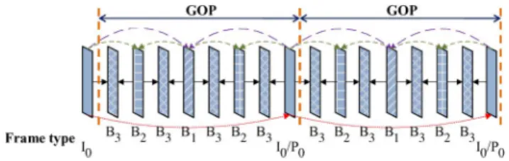
Currently, the temporal scalability in JSVM [6] is realized by using dyadic hierarchical prediction [7], [8]. A set of suc-cessive images is grouped into the so-called Group of Pictures (GOP), of which the size is typically power of two. A tem-poral scalable bit-stream is composed of one temtem-poral base layer and one or more temporal enhancement layers. For example, if the GOP size is , then its structure consists of the temporal base layer and temporal enhancement layers, denoted as . The last frame of each GOP is an anchor frame. The anchor frames form the temporal base layer ; they are coded as either I- or P-frame. The remaining frames, all lo-cated at the temporal enhancement layers, are coded as the hier-archical-B frames. Moreover, the BI operation is restricted to take the weighted sum of one preceding and one succeeding reference frames for prediction. Such a coding mechanism is referred to as the hierarchical-B prediction structure. Fig. 1 demonstrates an example of hierarchical-B prediction structure with , where the notation in frame type de-notes the frame is -type and located at tem-poral layer . Moreover, a B-frame takes a past frame and/or a future frame as its reference(s), both of which are equally dis-tant from this B-frame.
Fig. 1. Hierarchical-B prediction structure .
Temporal scalability made by the dyadic hierarchical-B prediction provides a high compression quality. In comparison to the commonly adopted IBBP and IPPP coding structures, the Y-PSNR can be averagely improved by at least 1.0 dB and 2.0 dB, respectively. Moreover, in this structure, experiments show that each reference list containing only one reference frame is sufficient. Empirically, the maximum coding efficiency occurs when the GOP size is between 8 and 32, as reported in [5].
B. Temporal Prediction Type Selection
To ensure the high compression performance, the SVC en-coder has to choose the most suitable block partition (mode) that leads to the optimal tradeoff between distortion and bit-rate by the Lagrange multiplier method [33]–[35]. Typically, two major nested processes are fully checked to obtain the optimal coding parameters: one is the block mode and the other is the temporal prediction type.
If a specific block mode with size (in pixel) is applied to an MB, there are sub-blocks inside this MB. Each sub-block needs to find its best temporal prediction type . This is done typically by performing the rate-constrained motion estimation that minimizes the RD cost :
(1) where
denotes the set of the uni-directional temporal predictions {FW, BW}, is the Lagrange multiplier for the rate-constrained motion estimation (a commonly used formulation is [33]–[35]),
is the pixel distortion, usually, the sum of absolute difference (SAD) using two MVs given by
(2)
is the sub-block (pixel set) specified by mode , is the predictive motion vector (pmv) generated by an MV predictor, (Typically, it is the median of the neighboring MVs.) denotes the number of bits representing the difference between and the motion
vector ( and/or
),
is the current frame pixel value, and are the pixel values of the
forwardly and the backwardly reconstructed frames, respectively.
The JSVM encoder [6] splits the selecting process of tem-poral prediction types into two stages, consisting of two uni-di-rectional predictions (FW and BW) and one bi-diuni-di-rectional pre-diction (BI).
• First stage (FW and BW): The motion-compensated pre-diction attempts to find the motions and by minimizing the costs and , separately. In com-puting (2), we first set and thus
for finding the FW MV; and then set and thus in the case of BW.
• Second stage (BI): As mentioned in [36], the motion vectors found by FW and BW are sub-optimal for BI. Therefore, the JSVM encoder [6] adopts an iterative approach to find the optimal MV pair for BI, denoted as and , by taking and as the initial search points. For example, the iterative process first locally refines with fixed. Then, is refined with fixed in the next iteration. The detailed analysis of this iterative approach is referred to [36]. During each iteration, the JSVM encoder performs the local refinement by an exhaustive search with a much smaller search range than that in . Furthermore, the iterative process is termi-nated if the in the current iteration is not better than that in the previous one. On the average, it results in about 2.3 BI iterations per MB (or sub-block). Note that the distortion in (2) computes the difference between the current MB and the average of two reference MBs by setting ,
, and .
Finally, three sets of distortions and motion bit-rate cost are collected and compared to produce the best RD costs and . For example, there are two sub-blocks in the block mode 16 8. Each of them has its best temporal prediction type and, say, one is FW and the other is BI. Then, each of them performs the reconstruction process to produce the RD performance of this 16 8 block mode. Next, we pick up the 8 8 mode and there are thus 4 sub-blocks. The MV search process is repeated for each sub-block and at the end we obtain the RD cost of this 8 8 mode. We try all possible modes and finally, we compare all these candidate modes and select the least RD cost block mode .
TABLE I
COMPLEXITYRATIOCOMPARED TOIPPP (FOR AGOP)
Average CPU time using , 35, 30, 25; JSVM 9.11 [6] with the encoding parameters in Table VII.
Platform: Athlon 3800+, 64-bit, dual-core processors, 2.0 GB RAM with Windows XP
C. Complexity Analysis
As discussed earlier, by allowing three temporal prediction types (FW, BW, and BI), the dyadic hierarchical-B prediction offers a high compression efficiency. However, its accompa-nying penalty is the very large amount of computation. Our statistics, collected from 9 sequences with four selected values, show very intensive computations in two prediction structures; one is the hierarchical-B prediction structure (FW, BW and BI), and the other is only. As listed in Table I, the complexity increases as the GOP size goes up. The increased computation is related to the percentage of frames (inside a GOP) that use multiple temporal prediction types. For example, there are of frames (in percentage) also use BW (and BI) for . Therefore, a hierarchical prediction structure using a large GOP size results in more computations.
On the average, as compared to the IPPP coding structure, the hierarchical-B prediction structure introduces additional 240% computations and the uni-prediction structure ( only) needs only about extra 55% encoding time. More specifically, the complexity ratio of and the BI is as follows:
Although the complexity of the uni-prediction structure ( only) is much lower than that of hierarchical-B prediction, the
only structure has a coding penalty of about 0.2 dB PSNR drop and 5% bit-rate increase. Thus, the BI type prediction is helpful in improving the RD performance but it consumes more than half of the encoding time. In this study we propose efficient methods to eliminate the unnecessarily computational load in calculating BI and to maintain a similar level of coded picture quality at the same time.
III. STATISTICALCHARACTERISTICS OFTEMPORAL
PREDICTION ATTEMPORALENHANCEMENTLAYERS
In this section, we investigate the statistical correlations of three temporal prediction types (FW, BW, and BI) at the SVC temporal enhancement layers. In order to study these correlations, our strategy is to collect the coding information by applying the exhaustive search on uni- and bi-directional predictions before the optimal partition size is determined. In Section III-A, we examine the prediction type distributions and their inheritances in the hierarchical blocks from large parti-tions to small ones. Then, Section III-B analyzes the relative coding efficiency contributed by the BI. In terms of the RD costs and the motion bit-rate costs, the last subsection explores their correlations between and BI. These statistical analyses are conducted based on encoding one temporal base layer with four temporal enhancement layers ; that is, the GOP size is 16. To evaluate the impact, two values, 30 and 40, are tested in experiments. The training set contains nine MPEG test videos
Due to limited space, we mainly show the statistical data of the CIF videos and the mean values (“MEAN”), which repre-sent the average behavior of these nine videos. In addition, the B-Skip mode calculates the predicted motion vectors to estimate its cost without actually performing the motion estimation op-eration. The estimated cost is used to compete with the other inter modes in making decision (on the optimal block size). Therefore, the B-Skip statistics are excluded from the following analysis.
A. Inheritance of Temporal Prediction Types
In this subsection, we collect the probability distributions of various temporal prediction types.
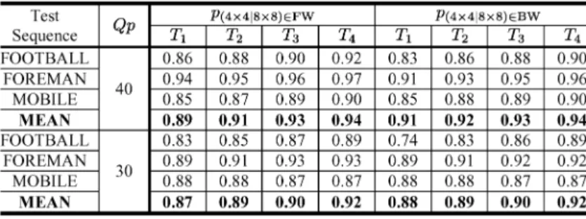
1) Prediction Type Distributions: We first gather the proba-bility distributions of temporal prediction types used in several distinct block partitions at various temporal enhancement layers and at different values. In any temporal layer of the hierar-chical-B prediction structure, the temporally forward and back-ward reference frames have equal distance away from the cur-rent frame. If the objects move at a constant speed, the curcur-rent MB can find its shifted version in either the forward reference or the backward reference. It implies that the selections of FW and BW are nearly equally likely, as shown in Fig. 2 for, partic-ularly, the MOBILE sequence.
The selection of BI is highly dependent on the video con-tent and the values, especially when the block partitions are larger than 8 8. Also, BI is selected more often at the high bit-rates (small ) because the encoder has sufficient bits to reduce the reconstruction distortion. In the MOBILE sequence, the BI probability of the 16 16 partition reaches about 80% at the low temporal enhancement layers, but its probability de-creases to 20% or less at the high temporal layers. In Fig. 2(c), BI is generally favored at large partitions (16 16 or 16 8) because BI offers more accurate motion compensation at a small MV bit-rate overhead. Clearly, distant reference frames
TABLE II
CONDITIONALPROBABILITIES OF ,AND
Fig. 2. Distribution of temporal prediction types (FW, BW, and BI). (a) FOOT-BALL; (b) MOBILE; (c) MEAN.
reduce the motion compensation effectiveness. Therefore, BI percentage goes down drastically at higher temporal layers. On the other hand, BI needs to transmit more MVs, twice as many as those of the FW/BW. If the reduced distortion provided by BI cannot compensate for the increased motion bit-rate cost, the BI type is not chosen. This is particularly true in the case of small blocks (4 4, 8 8). Therefore, at the same temporal enhancement layer, larger partitions prefer BI, especially in the complex-textured sequence MOBILE.
In summary, BI benefits the 16 16 and
partitions at the lower temporal enhancement layers, but for the small partitions from 8 8 down to 4 4, BI is seldom selected. This observation does not seem to be strongly affected by the video contents and the coding bit-rates.
2) Elimination of BI for Large Partitions: Our second obser-vation focuses on the use of BI in the parti-tions. As discussed in Section III-A-1, the BI probability in these partitions is much smaller than that in the 16 16 block size. That is, for instance, is less than
, which implies . In
order to find out whether or not these two groups
and overlap with each other, we consider three conditional probabilities defined below:
In Table II, these three conditional probabilities are higher than 80% in all cases and are about 95% on average. Moreover, their total probability is very close to one at higher temporal enhancement layers. This strong correlation indicates that the uni-direction prediction types are inheritable from the 16 16 partition to partitions. Thus, the information of the prior evaluation on 16 16 BI can provide a very reliable estimate to the use of BI for the partitions at both low and high bit-rates. We can quite confidently eliminate the use of BI in those partitions.
3) Consistency of FW and BW in Small Partitions: We now look into the block partitions smaller than 8 8. We find that we only need to evaluate the set ; also, the temporal prediction types of the 8 8 partition are strongly correlated to those of the 4 4 partition. As discussed in Section III-A-1, the probabilities of using BI for the 8 8 and the smaller partitions are often less than 20% and 10%, respectively. We collect the following two conditional probabilities of using FW and BW types. One is
defined by ,
which is equivalent to
.
Typically, the term is less than
2% in our collected data. The probability can
thus be approximated by .
Sim-ilarly defined is close to
. Experiments show that the approximated values of and are fairly close to data in Table III. Moreover, these two conditional probabilities slightly increase at higher temporal enhancement layers, except for the MOBILE sequence with , of which the correlations are rather similar for all temporal enhancement layers. Averagely, the consistency in selecting the same prediction direction can be up to 90%. Thus, the 8 8 prediction mode information serves as a good reference to its smaller partitions.
B. Rate-Distortion Contribution by BI
In this subsection, we address the relative RD improvement offered by BI in different block modes. As investigated before, the hierarchical-B prediction structure takes the advantage of
TABLE III
CONDITIONALPROBABILITIES OF AND
TABLE IV
AVERAGE FOR16 16, 8 8,AND4 4 BLOCKS INEACH TEMPORALENHANCEMENTLAYER(INPERCENTAGE)
using three temporal prediction types to improve the coding efficiency. According to the rate-distortion theory, a temporal prediction type with smaller RD cost provides better coding ef-ficiency. We adopt the RD cost function defined by JSVM [6] (which came from essentially the rate distortion theory) and col-lect all , , and for three squared-shape partitions, 16 16, 8 8, and 4 4. For each sub-block , we define the relative RD improvement , offered by the best temporal prediction type , as follows:
(3) The overall relative RD improvement is the sum of of
all sub-blocks; that is, , where
. Furthermore, in order to quantitatively determine the coding efficiency of using BI in the squared blocks, we define a BI performance index by
(4) In other words, the index , ranging from 0 to 1, indicates the percentage of the relative RD improvement contributed by BI for the totality of an size block. Moreover, a large value shows that the BI has a significantly relative im-provement in and that the BI should not be skipped.
Fig. 3 depicts the performance index value for each hierar-chical-B frame. As shown, the relative improvement offered by BI at high bit-rates is superior to that at low bit-rates because the encoder has more bits to reduce the distortion. This superi-ority at different bit-rates is particularly noticeable in the large 16 16 partition. On the other hand, the BI type usually fur-nishes less than 20% improvement on and , even at high coding rates.
Fig. 3. Measure index for individual hierarchical-B frame.
Table IV shows the average benefits offered by the BI type at various temporal enhancement layers. As illustrated, the per-formance index values decrease as the partition becomes finer. The has relatively average values of 24% and 57% for and , respectively; that is, BI plays an im-portant role in improving coding efficiency for large partitions. For the 8 8 partition, the effect of BI plunges to 11% on av-erage, which says that the set is sufficient to provide a good compression. Furthermore, when the partition is getting finer down to 4 4, the contribution of BI can be ignored because is less than 3% typically. However, some test videos such as MOBILE need BI can achieve better RD performance for both 16 16 and 8 8 partitions, because its and values reach 88.6% and 40.0%, respectively. In conclusion, the BI prediction type offers little coding gain for the block parti-tions smaller than 8 8.
C. Rate-Distortion Relationships Between Uni-Directional Predictions and biDirectional Prediction
In this subsection, we are interested in the relationships be-tween and BI in motion bit-rate cost and residual distortion. We collect the following information in our experiments: (a) the motion vector (MV) difference, (b) the motion bit-rate cost , and (c) the distortion for the three temporal prediction types.
Fig. 4. PDFs and CDFs of the vector difference . (a) FOOTBALL; (b) MO-BILE; (c) MEAN.
The statistical observations and theoretical analyses on the ex-perimental results are reported below.
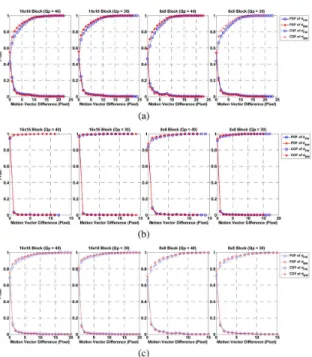
1) Motion Vector Difference: In order to find the correlations of two cost terms and between these temporal predic-tion types, we examine the MV differences after the MVs are refined by the BI search process. We look at two square block partitions, 16 16 and 8 8. On the JSVM 9.11 platform [6], we search for the best MVs of different prediction types for a specified block partition . Their notations are as follows:
As described earlier, the BI search process takes and as its initial search points for motion estimation. The Euclidean dis-tance is used to measure the MV difference and
(5) We statistically gather the 16 16 and 8 8 blocks that choose BI as their best temporal prediction type for generating the probability distributions (PDF) and cumulative probabili-ties (CDF) of and , as shown in Fig. 4. As shown, the PDFs of the MV difference are strongly clustered around the starting search points. Particularly, the one-pixel probability is close to 90% for the MOBILE. That is, most of the MVs after locally refined by BI are still very close to and . Typically, the MV differences are within three pixels; the CDFs of MV differences less than three pixels usually reach 80% or more. Our experiments show that
Fig. 5. Distributions of motion bit-rate cost. (a) 16 16 partition size with ; (b) 8 8 partition size with .
different block partitions have similar probability distributions. The similarity in the two motion pairs
and is the foundation of the following analysis.
2) Motion Bit-Rate Cost: Our second study tries to iden-tify the correlation of the motion bit-rate costs between and BI. As discussed in Section III-C-1, the MVs,
and , produced by BI are often close to and , respectively. In addition, the motion bit-rate cost is pro-portional to the MV length. Based on those two observations, we anticipate that there exists a strong correlation in motion bit-rate cost between and BI. More specifically, since the BI opera-tion needs two MVs to fetch two reference blocks for predicopera-tion, we collect the motion bit-rate costs of three temporal prediction
types, , , and to find
out the relationship between and the combined cost of ,
denoted as .
As depicted in Fig. 5, the distributions of and are noticeably concentrated along a straight line; this high
corre-lation is foreseen because and
, as discussed earlier. This implies that
and . Therefore, we make use of the first-order regression to represent the motion bit-rate cost by . Here, the motion bit-rate cost is mod-eled as an affine function of . This regression for based on is thus formulated as
(6) where and are the regression parameters. Furthermore, ac-cording to the collected data, the term in the regression model is usually nearly zero because when
and when . The first-order model is
thus simplified to a linear function,
(7) Applying the least squares technique, we can thus determine the optimal value by
TABLE V
OPTIMAL VALUES FOR THELINEARREGRESSIONMODEL
As tabulated in Table V, the optimal for 16 16 and 8 8 block partitions is around 0.93 and it slightly decreases at the higher temporal enhancement layers. Different block par-titions have similar slope values. This linear model,
, is a rather good approximation to the real because the percentage error is 11.3%. Here, in this linear regression model is 0.93, which is the av-erage value of MEAN.
3) Distortion Relationship: Our last study addresses on the correlations in the distortions of different prediction types. We obtain an upper bound of and will construct an approxi-mated distribution of (denoted as ).
For a given partition mode, the SAD metric used to evaluate its distortions of is defined by (2), unfolded as
(9) The distortion is calculated by two nested summations over and , is the current block, is the reference block in the direction, and
are the components of . Furthermore, each prediction error denotes its corresponding location in the block
differ-ence, . In the BI case with
equal weighted prediction, its distortion value is defined by
(10) Because the MVs finally adopted by BI are close to those produced by , the value of may be approximated by
, namely
(11)
As shown below, the average of can be derived as an upper bound of by using the well-known triangle inequality.
(12) In addition to derive an upper bound of , we verify that the probability distribution of is a Gamma distribution as described in the Appendix. The statistical tests indicate that the pair of tends to be bivariate-Laplacian distributed. This distribution model is used to construct a set of adaptive thresholds in Section IV.
IV. PROPOSEDFASTTEMPORAL PREDICTION
SELECTIONALGORITHM
In this section, we develop a fast temporal prediction type selection algorithm for the dyadic hierarchical-B prediction structure based on the observations in Section III. We derive a set of adaptive thresholds that efficiently eliminate unnecessary BI evaluations in Section IV-A. Then, combined with the adaptive thresholds, our proposed schemes are elaborated in Section IV-B.
A. Adaptive Thresholds
The highly correlated motion bit-rate costs and distortions be-tween and BI are used to develop a set of thresholds for block partitions from 16 16 to 8 8. According to the infor-mation obtained from the FW and BW processes, we can build a BI motion bit-rate cost estimator and a BI distortion estimator for a specified block.
As analyzed earlier, the motion bit-rate costs of
and are related by a linear regression model; that is, an es-timated motion bit-rate cost of BI, , is modeled as
. Moreover, among different block sizes, the op-timal slope does not change much, which ranges from 0.86 to 0.97. Hence, the mean value of of all block partitions (sizes) is adequate for all cases in estimating the motion bit-rate cost .
Next, we try to estimate from the probability model of and the percentage of the exception case of . Occasionally, is not an upper bound of if the chosen BI is inferior in terms of distortion. (Note that the MV chosen by BI is judged by its better combined RD value, not by the distortion value only.) From our collected data, the
ex-ception is 1% 5% on the average for
TABLE VI VALUES AND VALUES
As a consequence of the preceding discussions, the mean value of 1is sufficient to represent , namely, the es-timated distortion is
(13) As discussed earlier, (Normally,
indicates that the MV refinement in BI is effective.) and 5 for dif-ferent block sizes. The probability
can be calculated for a fixed . Therefore, we can de-termine the relationship between and without any knowledge of , as listed in Table VI. For example, the
probability is 3.6% from
our experimental data.
(14) From the above, we can derive
where denotes the inverse CDF of . Furthermore, it yields
(15) Finally, using the definition in Table VI, an estimate of (for the partition mode) is represented by
(16)
In addition, the percentage error is
around 12.5%.
B. Algorithm Overview
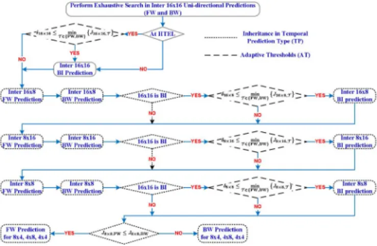
The flowchart in Fig. 6 depicts our proposed algorithm on eliminating the futile BI calculations. It mainly consists of two early termination criterions. First, a part of ineffective BI is skipped by the strong consistency in the temporal prediction types of large partitions. Then, the remaining unnecessary BI can be further detected by making use of the adaptive thresh-olds. The proposed approaches are split into three major stages, described below.
Stage 1: Conditionally Exhaustive Temporal Prediction Type Search for Inter16 16. The Inter16 16 partition
1The notation represents the Gamma distribution, where is the shape parameter and is the scale parameter.
Fig. 6. Selection algorithm for temporal prediction types.
mode conditionally checks all FW, BW, and BI types to identify its best temporal prediction type to be used in the Stage 2.
Step 1.1: Exhaustive Search on Uni-directional Pre-dictions. For the current MB, the set is evaluated in order to collect their distortions ( and ) and motion bit-rate costs ( and ) that will be used in Step 1.3. If the MB is located in the two highest temporal enhancement layers ( and ), denoted as HTEL, go to Step 1.3; otherwise, go to Step 1.2.
Step 1.2: BI Evaluation at Lower Temporal En-hancement Layers. At the temporal enEn-hancement
layers , the BI is always tested. Go to Stage 2.
Step 1.3: Conditional BI Execution at Higher Tem-poral Enhancement Layers. Using the information
obtained from Step 1.1, the threshold can be obtained by
(17)
If these two conditions and
are satisfied, the BI process is performed. Otherwise, BI is judged ineffective and thus skipped. Go to Stage 2.
Stage 2: Early Termination on BI for Large Partitions.
Before entering the Stage 2, the best temporal prediction type is determined in Stage 1. Two steps of this stage predict whether or not the BI type in
partitions have an inferior RD performance and thus can be excluded from testing. Section IV-B-1 details the early termination procedure.
Step 2.1: Exhaustive Uni-directional Prediction Type Search for Partitions . To gather the distortions ( and ) and mo-tion bit-rate costs ( and ) of partitions
Step 2.2: Pre-decided BI Elimination for Partitions
. If the pre-determined information is not BI, go to Stage 3. Otherwise, continue.
Step 2.3: Provisory BI Expulsion by Adaptive Thresholds. Similar to Step 1.3, the adaptive
thresh-olds are obtained by
(18)
where . The BI type
is calculated if the specifications
and are both true. Otherwise, the BI type is discarded.
Stage 3: Adaptive Prediction Type Selection for Small Partitions. Due to the strong correlation between the
pre-diction type of 8 8 and those of the smaller partitions, we can skip the less probable prediction types by checking the 8 8 prediction type. The Section IV-B-2 elaborates our implementation.
1) Early Termination on BI for Large Partitions: Based on our observations discussed earlier, the prediction type infor-mation of Inter16 16 partition mode is useful in skipping the BI type for large block partitions. More precisely, the
con-ditional probabilities, , , and
, can suggest whether the unnecessary compu-tations of BI of partitions can be avoided if the 16 16 partition is of the BI type. Thus, in Step 2.2, the saved computations in BI for large partitions depend on the BI selection rate for the 16 16 partition. Furthermore, for the case that is BI, the remaining superfluous BI can be detected by the thresholds in Step 2.3.
2) Adaptive Prediction Type Selection for Small Partitions: As suggested by our previous analysis for small partitions, we notice that (a) 10% blocks or less are coded with BI, (b) BI con-tributes less in improving compression efficiency as compared to , and (c) small partitions often have the same prediction types as that of their inherited 8 8 parent block. These three observations help us in developing an adaptive prediction selec-tion algorithm for small partiselec-tions.
The 8 8 or smaller blocks are seldom coded with BI. As discussed earlier, the prediction type of a smaller partition can be reliably estimated by its 8 8 parent partition. Thus, each smaller partition refined from an 8 8 partition only needs to check one prediction type. Furthermore, the candidate can be well predicted by comparing the and of its associ-ated 8 8 partition, even if its BI is not calculated in Stage 2. Therefore, in Stage 3, reduction in computation for small parti-tions can be achieved by skipping either FW or BW.
V. EXPERIMENTALRESULTS ANDDISCUSSIONS
A. Test Conditions
For performance assessment, we have implemented the pro-posed algorithms in JSVM 9.11 [6] and have tested 19 typical video sequences in four resolutions (QCIF/CIF/4CIF/HD for-mats), covering a broad range of visual characteristics. Our pro-posed schemes focus on the complexity reduction at the
tem-TABLE VII TESTINGCONDITIONS
poral enhancement layers in the dyadic hierarchical-B predic-tion structure. The detailed encoder parameters are given in Table VII and the other parameters are the default values set by the reference software JSVM 9.11 [6].
B. Performance Measures
To show the change in RD performance, we adopt the Bjontegaard metric [37], [38], which needs four RD points to measure the averaged Y-PSNR [BDP (dB)] and bit-rate differences [BDR (%)] between the two RD curves pro-duced by JSVM 9.11 [6] and by our schemes, respectively. Hence, we separate eight values into two sets, denoted by and , to measure the average RD perfor-mance for a wide range of bit-rates. These two sets
are and
To measure the average speedup performance at these eight RD test points, we define time saving (TS) for the whole encoding process and the complexity reduction on the hierar-chical-B frame process only.
1) The overall time saving is defined as
(19)
where and denotes the
en-coding time of JSVM 9.11 [6] and that of our schemes with quantization parameter , respectively. The nota-tion is the number of elements in the set . 2) In this measure, the denominator
is the additional computing time due to the use of hierarchical-B frames, compared to the
TABLE VIII
TIMESAVINGCONTRIBUTED BYTPANDAT (AVERAGEDFROM TO )
low-delay IPPP coding structure. Similarly, the numerator is the additional computing time of using our fast algo-rithms, shown in (20) at the bottom of the page, where represents the encoding time of JSVM 9.11 [6] with the IPPP coding structure and quantization parameter . Thus, represents how much additional encoding time our approach needs (compared to the IPPP coding structure).
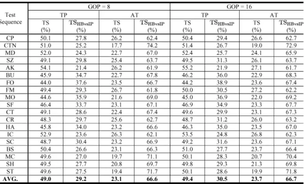
C. Performance Comparison With JSVM
Table VIII and Table IX present the time savings of the proposed schemes in comparison with JSVM 9.11. Listed in Table VIII are the improvements contributed by the inheritance of temporal prediction type (TP) and the adaptive thresholds to eliminate the superfluous BI computation (AT), respectively. The results are obtained by comparing the running time of the encoder with the following configurations:
Setting #1: JSVM 9.11 versus JSVM 9.11+TP: The TP set-ting makes use of the information produced by the 16 16 partition size to skip the BI type in the
partitions. For the block sizes smaller than 8 8, they only evaluate one of the uni-directional predictions, depending on the encoding information of 8 8.
Setting #2: JSVM 9.11 versus JSVM 9.11+AT: The AT setting uses the adaptive thresholds to conditionally select the BI type within the candidate set in the block partitions from 16 6 to 8 8 after performing FW and BW.
It can be seen that enabling the TP alone can averagely re-duce the overall running time by 50%, equivalent to a speedup of about 2 , whereas the AT offers only a moderate time saving of 17% 27%. Because the TP setting considers the temporal prediction selection in all block modes, it provides more com-plexity reduction, as compared to the AT setting. Interestingly, the results are similar regardless of the GOP size.
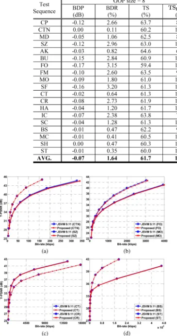
To see their combined effects, Table IX provides the time sav-ings relative to the exhaustive search, with both TP and AT en-abled. The results given in these two tables correspond to two GOP sizes: 8 and 16. As can be seen, when the TP is cou-pled with the AT, an average saving of 62% for the overall en-coding time is achieved. In other words, we can observe an ap-proximated 3 speedup. The improvement is achieved with a minor change in both bit-rate and Y-PSNR, as confirmed by the BDP/BDR values in the tables and the RD curves in Fig. 7. As discussed before, the BI examination in the encoding time is
about . That is, the improvement in
is generally limited to 55% when the BI computations are all skipped. However, our method can go beyond this limit, because in our algorithm the small partitions keep only one temporal prediction from for evaluation. Furthermore, the
values demonstrate that the additional computation required by the hierarchical-B prediction structure can be averagely reduced by 89%. (The average is around 11%.)
The overall time savings in Table IX are not the sum of the results from Table VIII. In our approach, we set two
TABLE IX
PERFORMANCECOMPARISONSWITHJSVM 9.11 [6]
Fig. 7. Comparisons in RD curve . (a) QCIF; (b) CIF; (c) 4CIF; (d) HD (720p).
sive criterions to conditionally eliminate the BI computation, as illustrated in Fig. 6; one is TP, and the other is AT. However, their contributions are overlapped for some MBs; that is, if these MBs satisfy the first TP criterion, the AT criterion is not active in our design flowchart. Hence, with the average time saving of 50% by the TP, the AT criterion can additionally provide about 12% improvement. The additional improvement comes from the cases when the 16 16 partition is not BI, and the AT condi-tion is satisfied. For example, in Fig. 2(a), about 70% of MBs do not select BI at (with ) when 16 16 partition is examined. In this case, our algorithm skips these 70% of BI calculations. In total, there are 85% of 16 8 partitions do not prefer BI in our collected data. Therefore, only the remaining
15% of 16 8 partition blocks are further checked by the AT criterion for further complexity reduction.
Moreover, in Table X, the overall time saving decreases as the value becomes small. The complexity reduction goes down from 67% to 48% as decreases. This is due to the combined
RD cost that affects the
selec-tion of temporal predicselec-tion type. Such an optimizaselec-tion principle tends to cut down the motion bit-rate term when is large. On the other hand, because of the abundant bit budget, this opti-mization process spends more bits to reduce the distortion term
at a small . Thus, BI is used more often for small values because BI is effective in reducing the distortion. Hence, fewer BI blocks can be skipped by our approach.
D. Performance Comparison With Other Fast Algorithms In addition to the exhaustive search, we also compare our ap-proaches with two well recognized fast algorithms, Li’s method [29] and Lee’s method [30]; both save the computing time based on mode reduction. Therefore, our approach is very different from theirs. Nevertheless, for comparison purpose, the same en-coding configuration and test videos (Table VII) are used in the experiment (on JSVM 9.11).
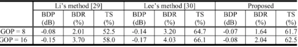
As shown in Table XI, the Li’s method [29] can averagely achieve about 55% time reduction and has a Y-PSNR loss of 0.11 dB and 2.8% bit-rate increase. The Lee’s method [30] has the best time saving at about 65%, but it has also the highest coding quality loss, 0.15 dB Y-PSNR and 3.6% bits. Our scheme has roughly the least RD loss, 0.08 dB Y-PSNR and 1.8% bits, and its time saving is about 62%. If all are mea-sured in ratio, our time saving is better than [29] by about 10% with a slightly better RD quality. And our time saving is slightly worse than [30] by 5% but both the PSNR and the bit rate losses are 50% better. However, we like to point out that our approach, focusing on the temporal prediction type reduction, is very dif-ferent from the fast mode decision schemes in [29] and [30]. In
TABLE X
AVERAGETIMESAVING FORTWOGOP SIZES, 8AND16, WITHVARIOUS VALUES
TABLE XI
PERFORMANCECOMPARISONS(AVERAGEBDP, BDR,ANDTS)
other words, we are not aiming at the same target; in contrast, our scheme may be combined with these schemes to achieve further complexity reduction. Simulations also indicate that our scheme is not sensitive to the video variation. Thus, instead of mode selection, reducing candidates in temporal prediction can be a promising approach for decreasing complexity in the hier-archical-B prediction structure.
VI. CONCLUSIONS
In this paper, we propose an effective temporal prediction type selection algorithm for the dyadic hierarchical-B predic-tion structure in SVC [4], [5], in which the unnecessary BI cal-culations are skipped for large block partitions and only one of the uni-directional temporal predictions is calculated for small partitions. The techniques used are (a) conditional elimination of BI for large partitions, (b) adaptive thresholds produced by the information obtained in the FW and BW processes, and (c) adaptive selection of FW and BW for small partitions. We first perform the uni-directional temporal predictions, FW and BW. Then, we make use of the strong correlations in the inher-itance of temporal predictions and also construct a set of adap-tive thresholds, both of which decide the BI operation is to be performed or not. To construct a reliable threshold, we examine the correlations of motion bit-rate costs and the distortions be-tween the uni-directional temporal predictions and the BI type. Also, our statistical analysis shows that BI in small partitions does not contribute much in improving compression efficiency.
These findings in the temporal enhancement layers are intelli-gently used for accelerating the encoding process.
On the average, our scheme can demonstrate up to 65.3% complexity reduction for the entire encoding process with minor changes in coding efficiency, as compared to JSVM 9.11 [6]. Also, the extra computations in the hierarchical-B prediction can be reduced by up to 93.9%. Hence, our approach can achieve a similar coding performance of JSVM 9.11 [6] but with much lower computational complexity. Moreover, our fast algorithm only reduces the complexity in temporal prediction types without any a priori mode reduction and can be applied to all enhancement coding layers.
APPENDIX
In Section III-C-3, we have derived the upper bound of , as shown in (A.1). In addition, we further study its probability distribution in this appendix.
(A.1) Ideally the FW and BW operations can find the shifted ver-sion of the current block if there are no quantization error and noise in the reference frames. As a result, most correlations be-tween frames can be removed by the inter prediction, except for
the prediction error term, composed of the quantization error and noise. Typically, the prediction error from FW and BW is nearly Laplacian distributed, as reported in [39]. Hence, we assume that the ’s inside a block have the i.i.d. Laplacian distribution, and so do the ’s. Also, we assume the data in one block have the same statistical parameters such as mean and variance.
Next, for a specific location , we like to show that the and pair is jointly Laplacian. Note that al-though two random variables and are marginally Lapla-cian-distributed, it does not imply the pair is jointly Laplacian. We adopt a popular goodness-of-fit test to examine the distribution of . It is the Pearson’s -test
Chi-square test: The -test divides the data range into mutually exclusive and exhaustive intervals (events), denoted by . The -test statistic is defined as [40]
(A.2) where is the total number of data samples in a block, is the observed frequency (number of samples) of the event , and is the expected value of the event ( is the model probability of event ). Essentially, the
-test statistic shows the difference between the empirical frequencies and the model-derived mean values.
These two tests measure the similarity between the collected observations and a chosen model distribution. We pick up the following two bivariate distributions to match our collected data.
Bivariate Gaussian distribution: The commonly used
bi-variate Gaussian distribution is defined as
(A.3) where two random variables and form the vector ,
is the expected value of , the covariance matrix , and is the correlation between and .
Bivariate Laplacian distribution: The bivariate
Lapla-cian distribution has heavier tails than the bivariate Gaussian distribution and its PDF is defined by [41]
(A.4) where is the modified Bessel function of the second kind.
In the data fitting process, we decide two parameters and by adopting the approach of method of moments [42], [43]. Again, the distribution parameters of each block are calculated individually because they may vary from block to block. After the parameters of these two bivariate PDF are determined, we evaluate how well they match the empirical data of pair
.
We examine this goodness-of-fit test in two distinct block sizes, 16 16 and 8 8. The empirical data are evaluated against these two selected model distributions. In Table A-I,
TABLE A-I
AVERAGE TEST-STATISTICVALUE FORTEMPORALENHANCEMENTLAYER
the reference model is better than the other model in terms of the -test statistic . The value of usually varies from 16 to 33, but the value of is about 60 on average. We thus conclude that the collected data are closer to the bivariate Laplacian distribution. We also use another goodness-of-fit test, Kolmogorov-Smirnov test (KS-test), and the conclusion is similar. Additional test data and discussions can be found in [44].
After we use the jointly Laplacian distribution to model , we can derive the distribution
of ;
namely, the distribution of . According to the property of Laplacian distribution [41], a linear combination is one-dimensional Laplacian distribution if and are jointly Laplacian. Hence, the term
(A.5) is also Laplacian distributed. Moreover, from the probability theory, the absolute value of a Laplacian distribution is expo-nentially distributed and the sum of i.i.d. exponential distribu-tions forms a gamma distribution, as shown below [45], [46].
(A.6)
Hence, should have a Gamma distribution , where is the shape parameter and is the scale parameter.
REFERENCES
[1] J.-R. Ohm, “Advances in scalable video coding,” Proc. IEEE, vol. 93, no. 1, pp. 42–56, Jan. 2005.
[2] Advanced Video Coding for Generic Audiovisual Services ITU-T H.264 (03/2010), Mar. 2010.
[3] T. Wiegand, G. Sullivan, G. Bjontegaard, and A. Luthra, “Overview of the H.264/AVC video coding standard,” IEEE Trans. Circuits Syst. Video Technol., vol. 13, no. 7, pp. 560–576, Jul. 2003.
[4] T. Wiegand, G. Sullivan, J. Reichel, H. Schwarz, and M. Wien, Joint Draft ITU-T Rec. H.264 | ISO/IEC 14496-10/Amd. 3 Scalable Video Coding ISO/IEC JTC1/SC29/WG11 and ITU-T SG16 Q.6, JVT-X201, Jun. 2007.
[5] H. Schwarz, D. Marpe, and T. Wiegand, “Overview of the scalable video coding extension of the H.264/AVC standard,” IEEE Trans. Cir-cuits Syst. Video Technol., vol. 17, no. 9, pp. 1103–1120, Sep. 2007.
[6] J. Reichel, H. Schwarz, and M. Wien, Joint Scalable Video Model JSVM-12 Text ISO/IEC JTC1/SC29/WG11 and ITU-T SG16 Q.6, JVT-Y202, Oct. 2007.
[7] H. Schwarz, D. Marpe, and T. Wiegand, Hierarchical B Pictures ISO/IEC JTC1/SC29/WG11 and ITU-T SG16 Q.6, JVT-P014, Jul. 2005.
[8] H. Schwarz, D. Marpe, and T. Wiegand, “Analysis of hierarchical B pictures and MCTF,” in IEEE Int. Conf. Multimedia Expo, 2006, pp. 1929–1932.
[9] T. Wiegand, X. Zhang, and B. Girod, “Long-term memory motion-compensated prediction,” IEEE Trans. Circuits Syst. Video Technol., vol. 9, no. 1, pp. 70–84, Jan. 1999.
[10] T.-Y. Kuo and H.-J. Lu, “Efficient reference frame selector for H.264,” IEEE Trans. Circuits Syst. Video Technol., vol. 18, no. 3, pp. 400–405, Mar. 2008.
[11] A. Chang, O. C. Au, and Y. M. Yeung, “A novel approach to fast multi-frame selection for H.264 video coding,” in Proc. IEEE Int. Conf. Acoust., Speech Signal Process., 2003, pp. III-413–III-416.
[12] Y. Su and M.-T. Sun, “Fast multiple reference frame motion estimation for H.264/AVC,” IEEE Trans. Circuits Syst. Video Technol., vol. 16, no. 3, pp. 447–452, 2006.
[13] S.-E. Lim, J.-K. Han, and J.-G. Kim, “An efficient scheme for motion estimation using multireference frames in H.264/AVC,” IEEE Trans. Multimedia, vol. 8, no. 3, pp. 457–466, Mar. 2006.
[14] M.-J. Chen, G.-L. Li, Y.-Y. Chiang, and C.-T. Hsu, “Fast multi-frame estimation algorithms by motion vector composition for the MPEG-4/AVC/H.264 standard,” IEEE Trans. Multimedia, vol. 8, no. 3, pp. 478–487, Mar. 2006.
[15] L. Shen, Z. Liu, Z. Zhang, and G. Wang, “An adaptive and fast multiframe selection algorithm for H.264 video coding,” IEEE Signal Process. Lett., vol. 14, no. 11, pp. 836–839, Nov, 2007.
[16] Huang et al., “Analysis and complexity reduction of multiple reference frames motion estimation in H.264/AVC,” IEEE Trans. Circuits Syst. Video Technol., vol. 16, no. 4, pp. 507–522, Apr. 2006.
[17] Z. Liu et al., “Motion feature and hadamard coefficients-based fast multiple reference frame motion estimation for H.264,” IEEE Trans. Circuits Syst. Video Technol., vol. 18, no. 5, pp. 620–632, May 2008.
[18] S.-H. Ri, Y. Vatis, and J. Ostermann, “Fast inter-mode decision in an H.264/AVC encoder using mode and lagrangian cost correlation,” IEEE Trans. Circuits Syst. Video Technol., vol. 19, no. 2, pp. 302–306, Feb. 2009.
[19] Y.-K. Tu, J.-F. Yang, and M.-T. Sun, “Efficient rate-distortion estima-tion for H.264/AVC coders,” IEEE Trans. Circuits Syst. Video Technol., vol. 16, no. 5, pp. 600–611, May 2006.
[20] K.-Y. Liao, J.-F. Yang, and M.-T. Sun, “Rate-distortion cost estimation for H.264/AVC,” IEEE Trans. Circuits Syst. Video Technol., vol. 20, no. 1, pp. 38–49, Jan. 2010.
[21] M. Paul, M. R. Frater, and J. F. Arnold, “An efficient mode selec-tion prior to the actual encoding for H.264/AVC encoder,” IEEE Trans. Multimedia, vol. 11, no. 4, pp. 581–588, Apr. 2009.
[22] A. C.-W. Yu, G. R. Martin, and H. Park, “Fast inter-mode selection in the H.264/AVC standard using a hierarchical decision process,” IEEE Trans. Circuits Syst. Video Technol., vol. 18, no. 2, pp. 186–195, Feb. 2008.
[23] H. Wang, S. Kwong, and C.-W. Kok, “An efficient mode decision al-gorithm for H.264/AVC encoding optimization,” IEEE Trans. Multi-media, vol. 9, no. 4, pp. 882–888, Apr. 2007.
[24] Y.-M. Lee and Y. Lin, “Zero-block mode decision algorithm for H.264/ AVC,” IEEE Trans. Image Process., vol. 18, no. 3, pp. 524–533, Mar. 2009.
[25] B.-G. Kim, “Novel inter-mode decision algorithm based on mac-roblock (MB) tracking for the P-slice in H.264/AVC video coding,” IEEE Trans. Circuits Syst. Video Technol., vol. 18, no. 2, pp. 273–279, 2008.
[26] H. Zeng, C. Cai, and K.-K. Ma, “Fast mode decision for H.264/AVC based on macroblock motion activity,” IEEE Trans. Circuits Syst. Video Technol., vol. 19, no. 4, pp. 1–10, Apr. 2009.
[27] L. Shen, Z. Liu, Z. Zhang, and X. Shi, “Fast inter mode decision using spatial property of motion field,” IEEE Trans. Multimedia, vol. 10, no. 6, pp. 1208–1214, 2008.
[28] Z. Liu, L. Shen, and Z. Zhang, “An efficient intermode decision al-gorithm based on motion homogeneity for H.264/AVC,” IEEE Trans. Circuits Syst. Video Technol., vol. 19, no. 1, pp. 128–132, Jan. 2009.
[29] H. Li, Z.-G. Li, and C. Wen, “Fast mode decision algorithm for inter-frame coding in fully scalable video coding,” IEEE Trans. Circuits Syst. Video Technol., vol. 16, no. 7, pp. 889–895, Jul. 2006.
[30] B. Lee et al., “An efficient block mode decision for temporal scala-bility in scalable video coding,” in Proc. SPIE, 2008, vol. 6822, pp. 68220L-1–68220L-9.
[31] H.-C. Lin, H.-M. Hang, and W.-H. Peng, “Fast temporal prediction selection for H.264/AVC scalable video coding,” in Proc. IEEE Int. Conf. Image Process., 2009, pp. 3425–3428.
[32] H.-C. Lin and H.-M. Hang, “Fast algorithm on selecting bi-directional prediction type in H.264/AVC scalable video coding,” in Proc. IEEE Int. Symp. Circuits Syst., 2010, pp. 113–116.
[33] G. Sullivan and T. Wiegand, “Rate-distortion optimization for video compression,” IEEE Signal Process. Mag., vol. 15, no. 6, pp. 74–90, 1998.
[34] T. Wiegand and B. Girod, “Lagrange multiplier selection in hybrid video coder control,” in Proc. IEEE Int. Conf. Image Process., 2001, vol. 3, pp. 542–545.
[35] T. Wiegand, H. Schwarz, A. Joch, and F. Kossentini, “Rate-constrained coder control and comparison of video coding standards,” IEEE Trans. Circuits Syst. Video Technol., vol. 13, no. 7, pp. 688–702, 2003. [36] M. Flierl, T. Wiegand, and B. Girod, “A locally optimal design
algo-rithm for block-based multi-hypothesis motion-compensated predic-tion,” in Proc. Data Compression Conf., 1998, pp. 239–248. [37] G. Bjontegaard, Calculation of Average PSNR Differences Between
RD-curves ISO/IEC JTC1/SC29/WG11 and ITU-T SG16 Q.6, Doc. VCEG-M33, Apr. 2001.
[38] S. Pateux and J. Jung, An Excel Add-in for Computing Bjontegaard metric and Its Evolution ISO/IEC JTC1/SC29/WG11 and ITU-T SG16 Q.6, Doc. VCEG-AE07, Jan. 2007.
[39] M. Narroschke, “Extending H.264/AVC by an Adaptive Coding of the Prediction Error,” in Proc. Picture Coding Symposium, 2006. [40] R. V. Hogg, J. W. McKean, and A. T. Craig, Introduction to
Mathematical Statistics, 6th ed. Englewood Cliffs, NJ: Prentice Hall, 2004.
[41] S. Kotz, T. J. Kozubowski, and K. Podgorski, The Laplace Distribution and Generalizations. New York: Birkhauser, 2001.
[42] S. M. Kay, Fundamentals of Statistical Signal Processing: Estimation Theory. Englewood Cliffs, NJ: Prentice-Hall, 1993, vol. I. [43] T. Sltoft, T. Kim, and T.-W. Lee, “On the multivariate laplace
distri-bution,” IEEE Signal Lett., vol. 13, no. 5, pp. 300–303, 2006. [44] H.-C. Lin, “Fast encoding algorithm design for H.264/MPEG-4 AVC
scalable video coding standard,” Ph.D. dissertation, NCTU, Taiwan, Jun. 2010.
[45] Laplace Distribution [Online]. Available: http://en.wikipedia.org/wiki/ Laplace_distribution
[46] Exponential Distribution [Online]. Available: http://en.wikipedia.org/ wiki/Exponential_distribution
Hung-Chih Lin was born in Nantou, Taiwan, in
1982. He received the B.S. degree in electrical control engineering in 2004, and the M.S. and Ph.D. degree in electronics engineering in 2005 and 2010, all from National Chiao-Tung University (NCTU), Hsinchu, Taiwan.
He currently serves as a senior engineer in MediaTek, Inc., Hsinchu, Taiwan. His work mainly focuses on software video encoder for real-time applications, specifically, encoder optimization using fast motion search and ARM-related SIMD operations. His research interests include numerical matrix computations, digital image/video processing, and scalable video compression. In particular, he specializes in fast algorithm designs and implementations. He has explored on the encoder optimization of the MPEG video coding standards since his M.S. program.
For outstanding accomplishments in these techniques, Dr. Lin received Ex-cellent Achievement Award of Ph.D. Dissertation from Department of Electrical Engineering, NCTU in 2010.
Hsueh-Ming Hang (F’02) received the B.S. and
M.S. degrees in control engineering and electronics engineering from National Chiao Tung University, Hsinchu, Taiwan, in 1978 and 1980, respectively, and Ph.D. in electrical engineering from Rensselaer Polytechnic Institute, Troy, NY, in 1984.
From 1984 to 1991, he was a Technical Staff Member with AT&T Bell Laboratories, Holmdel, NJ, and then he joined the Electronics Engineering Department of National Chiao Tung University (NCTU), Hsinchu, Taiwan, in 1991. From 2006 to 2009, he took a leave from NCTU and was appointed as Dean of the EECS College at National Taipei University of Technology, Taipei, Taiwan. He is currently a Distinguished Professor of the EE Dept and an Associate Dean of the ECE College, NCTU. He holds 13 patents in the U.S., China, and Japan, and has published over 170 technical papers related to image compression, signal processing. Since 1984, he has been actively involved in the international MPEG standards. His current research interests include multimedia compres-sion, image/signal processing algorithms and architectures, and multimedia communication systems.
Dr. Hang was an associate editor (AE) of the IEEE TRANSACTIONS ONIMAGE
PROCESSING(TIP, 1992–1994), the IEEE TRANSACTIONS ONCIRCUITS AND
SYSTEMS FORVIDEOTECHNOLOGY(1997–1999), and currently an AE of the IEEE TIP again. He is co-editor and contributor of the Handbook of Visual Com-munications published by Academic Press. He is a recipient of the IEEE Third Millennium Medal and is a Fellow of IEEE and IET and a member of Sigma Xi.
Wen-Hsiao Peng was born in HsinChu, Taiwan in
1975. He received his B.S., M.S., and Ph.D. degrees in Electronics Engineering from National Chiao Tung University (NCTU), Taiwan in 1997, 1999, and 2005, respectively.
From 2000–2001, he was with the Intel Micropro-cessor Research Laboratory, Santa Clara, U.S., where he developed the first real-time MPEG-4 fine gran-ularity scalability codec and demonstrated its appli-cation in a 3-D, peer-to-peer video conferencing. In 2005, he joined the Department of Computer Science, NCTU, where he is currently an Assistant Professor. Since 2003, he has actively participated in the International Organization for Standardization (ISO) Moving Picture Expert Group (MPEG) digital video coding standardization process and contributed to the development of MPEG-4 Part 10 AVC Amd.3 scalable video coding standard. He has published more than 30 technical papers in the field of video and signal processing. His current research interests include high-effi-ciency video coding, scalable video coding, video codec optimization, and plat-form-based architecture design for video compression.
Dr. Peng currently serves as a Technical Committee Member for “Visual Signal Processing and Communications” and “Multimedia Systems and Appli-cation” tracks for the IEEE Circuits and Systems Society. He organized two special sessions on High-Efficiency Video Coding in ICME 2010 and APSIPA ASC 2010, and served as a Technical Program Co-Chair for VCIP 2011.