基於顯著特性之靜態路標偵測與辨識系統

國 立 交 通 大 學

電子工程學系 電子研究所碩士班

碩

士

論

文

基於顯著特性之靜態路標偵測與辨識系統

Saliency-based Detection and Recognition of

Static Waymarks

研 究 生：林瑋國

指導教授：王聖智 博士

基於顯著特性之靜態路標偵測與辨識系統

Saliency-based Detection and Recognition of

Static Waymarks

研 究 生：林瑋國 Student：Wei-Guo Lin

指導教授：王聖智博士 Advisor：Dr. Sheng-Jyh Wang

國 立 交 通 大 學

電子工程學系 電子研究所碩士班

碩 士 論 文

A Thesis

Submitted to Department of Electronics Engineering & Institute of Electronics College of Electrical and Computer Engineering

National Chiao Tung University in partial Fulfillment of the Requirements

for the Degree of Master in

Electronics Engineering September 2010

Hsinchu, Taiwan, Republic of China

基於顯著特性之靜態路標偵測與辨識系統

研究生：林瑋國 指導教授：王聖智 博士

國立交通大學

電子工程學系 電子研究所碩士班

摘要

在本論文中，我們提出一套基於顯著特性之靜態路標偵測與辨識

系統，可在具有明顯路標的場景中被用來進行盲人路徑導航。在此系

統中，具有正常視力之輔助者事先取得某一場景之影片，並在影片中

圈選出具有 1)強烈對比、2)簡單紋理和 3)規則形狀等特性之顯著靜態

路標。利用這些特性，我們設計出顯著特性的偵測技術，使得此系統

日後可以在同樣的場景中，快速地從新拍攝到的影像中找尋出可能是

這些顯著靜態路標的候選區域來。而於這些候選區域中，本系統再利

用具有方向性的濾波器組合和擁有色調、飽和度和亮度的色彩空間，

分別分析形狀與顏色特徵，進而辨識出候選區域中是否有使用者原先

所圈選的靜態路標。在本論文中，我們透過仔細的分析研究，發展了

一套靜態路標偵測與辨識系統，並有效地解決了以下的幾項主要挑戰:

1)亮度變化、2)物體的縮放、3)旋轉、4)不同路標的形狀考量、以及

5)不平衡的訓練資料。

Saliency-based Detection and Recognition of

Static Waymarks

Student: Wei-Guo Lin Advisor: Dr. Sheng-Jyh Wang

Department of Electronics Engineering, Institute of Electronics

National Chiao Tung University

Abstract

In this thesis, we propose a saliency-based system for the detection

and recognition of static waymarks. This system can be used to help blind

people navigate through a scene with noticeable waymarks. In this system,

a user with normal vision first captures a video of the scene. He or she

then manually selects a few static waymarks in the video that possess the

following properties: 1) with strong contrast, 2) with simple texture, and

3) with regular shape. Based on these properties, we design a saliency

detector which can quickly identify the candidate regions in any newly

captured video. Over the candidate regions, the system adopts a set of

directional filter banks and the HSV color space to analyze the shape

features and the color features respectively for the recognition of the

pre-selected waymarks. In this thesis, through careful design and analysis,

we have developed a static waymark detector that can well handle the

challenges of varying illumination, scaling, rotation, shape variation, and

imbalanced training data.

誌謝

在此要特別感謝我的指導教授 王聖智老師，在他的細心指導下，學

習到了很多研究的方法與態度，除了課業上的知識外，也學習到許多

待人接物與處理事情的技巧，使我在這兩年中有著長足的成長。感謝

實驗室的全體夥伴，尤其是敬群學長、慈澄學長、禎宇學長、奕安學

長在我需要幫助時，給予我真誠的協助。同時，我也要感謝實驗夥伴

周節，在求學的路途上有你的陪伴與鼓勵讓我克服了許多困難。再

者，我要感謝堅柱和佳龍兩位同學在口試前不斷的訓練我演說技巧和

投影片修改，以及一路上關心和鼓勵我的朋友，因為有你們，使我變

得更堅強。最後，我也要感謝我的家人，因為有他們的支持，讓我可

以安心地在學業上努力。

Content

Chapter 3. Proposed Method ... 15

3.1. Bottom-Up ... 16

3.1.1. Linear Filtering of Image Data ... 17

3.1.2. Strong Contrast ... 17 3.1.3. Regular Shape ... 22 3.1.4. Simple Texture ... 23 3.1.5. Combination ... 24 3.2. Top-Down Learning ... 25 3.2.1. Color Analysis ... 25 3.2.2. Shape Analysis ... 26

3.2.3. Support Vector Machine ... 29

3.2.4. Synthetic Minority Over-sampling Technique (SMOTE) ... 31

Chapter 4. Experimental Results ... 33

List of Figures

Figure 1-1 Use waymarks to help blind people ... 2

Figure 2-1 Traffic signs in [1] ... 3

Figure 2-2 The flow chart of the system in [1] ... 4

Figure 2-3 (a) Original image (b) Segmented by red color (c)(d) Candidate blobs [1] . 5 Figure 2-4 DtBs for a triangular shape [2] ... 5

Figure 2-5 The interested regions for circular and triangular [1] ... 6

Figure 2-6 Five kinds of traffic signs in [2] (a) Speed limit sign (b) No stopping sign (c) No entry sign(d) Pedestrian sign (e) Parking sign ... 6

Figure 2-7 The traffic sign detection framework in [2] ... 7

Figure 2-8 (a) Original image. (b) Saliency map. (c) Traffic sign saliency regions (marked by green rectangles) [2] ... 7

Figure 2-9 (a) Example of illumination invariance.(b) Example of different scales[2]. 8 Figure 2-10 Proposed method of [6] ... 9

Figure 2-11 (a) Input image (b) corresponding saliency map ... 9

Figure 2-12 (a) Input image (b) corresponding log spectrum (c) reference (d) spectral residual ... 10

Figure 2-13 (a) Three input images (b) saliency map by[8] (c) saliency map by [7] . 10 Figure 2-14 The main idea of feature-pair ... 11

Figure 2-15 Example of intensity-pair distribution in [9] ... 11

Figure 2-16 (a) Input image (b) saliency map by [9] ... 12

Figure 2-17 Corner detection result in [3] ... 12

Figure 2-18 The relation of boundary line in [4] ... 13

Figure 2-19 (a) The Dbts of triangle (b) the feature vectors of (a) by Dtbs [5] ... 13

Figure 2-20 Three examples of SURF [10] ... 14

Figure 3-1 Block diagram of the proposed system ... 15

Figure 3-2 Block diagram of the proposed Bottom-up ... 16

Figure 3-3 The example of the static waymarks ... 17

Figure 3-4 The main idea of feature-pair ... 18

Figure 3-5 The feature-pair distribution ... 18

Figure 3-6 The example of R color-pair distribution ... 19

Figure 3-7 The 3-D histogram ... 20

Figure 3-8 The computation of edge weight ... 20

Figure 3-9 The 3-D histogram ... 21

Figure 3-10 The example of the static waymarks ... 22

Figure 3-11 The filter that can detect boundary [11] ... 22

Figure 3-13 (a) Blue band (b) B color of blue band ... 23

Figure 3-14 (a) Original signal(sine) (b) Reconstruction result using phase [8] .... 24

Figure 3-15 (a) Blue signboard (b) the saturation of (a) quantized by ten (c) hue of (a) quantized by ten ... 25

Figure 3-16 The six directional lines ... 26

Figure 3-17 The six directional filters ... 26

Figure 3-18 (a) Original (b) rotate ... 26

Figure 3-19 Maximum shift ... 27

Figure 3-20 (a) Find the maximum region (b) correspond region t (c) the result of shift ... 27

Figure 3-21 (a) Find the maximum region (b) correspond region t (c) the result of shift ... 28

Figure 3-22 Adjust the result of filters ... 28

Figure 3-23 The three hyper planes to separate two sets ... 29

Figure 3-24 Find the hyper plane ... 30

Figure 3-25 (a) Balanced data (b) imbalanced data ... 31

Figure 4-1 The overview of three places ... 33

Figure 4-2 Left to right: blue signboard, fire hydrant, Disabled signboard, and parking signboard ... 33

Figure 4-3 Use different colors bounding boxes for different static waymarks ... 34

Figure 4-4 Different scales of static waymarks in the afternoon ... 35

Figure 4-5 Static waymarks in the afternoon with rotation variations ... 35

Figure 4-6 Static waymarks at noon with rotation variations ... 36

Figure 4-7 Static waymarks in the evening with rotation variations ... 36

List of Tables

Table 4-1 Number of training images ... 34 Table 4-2 Detection rate and false alarm at different time for each static waymarks .. 37 Table 4-3 Detection rate and false alarm for different bottom-up methods ... 38 Table 4-4 Computing time for different bottom-up detection ... 38 Table 4-5 Detection rate and false alarm for three new places ... 39

1

Chapter 1.

I

NTRODUCTION

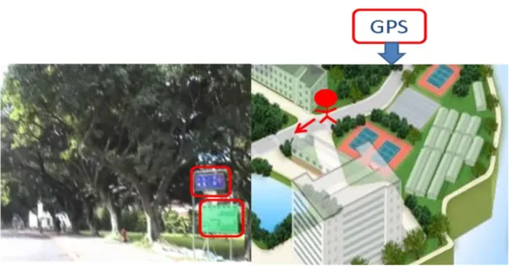
For blind people, it is very important for them to realize where they are or which direction they are heading for. The first solution people think is GPS (Global Positioning System), which can give the position of the user. However, for a user at a standstill, GPS can‟t offer the orientation information, which could be very crucial to blind people. Another method is to install sound devices around the path to offer sound service. A main drawback of this approach is the price to set up numerous sound devices along the path. A new approach is to use the street-view tool on web service. However, this requires a large data base and heavy computations for recognition.

One more approach is to use GPS plus salient waymarks, as shown in Figure 1-1. If a blind person uses GPS, he/she would know his/her location and the expected waymarks around him/her. If the blind person can carry a camera with him/her, together with a computational device to identify the location of waymarks in the captured images, he/she would be able to realize what direction his/her face is heading to. Hence, in this thesis, we aim to set up a system that can automatically detect and recognize salient waymarks in 2-D images.

2

Figure 1-1 Use waymarks to help blind people

Our system is designed to help a blind person to pass through a path that he/she frequently walk on. The implementation of this system includes four major steps: 1) an assistant with normal vision first captures a few videos along the regular route; 2) the assistant selects salient waymarks in the captured videos; 3) our algorithm learns the features of the selected waymarks; and 4) we develop a suitable detector to automatically identify these salient waymarks.

Here come a few challenges in the development of our system. The first and the most important challenge is the change of lighting condition. The other challenges are the scaling and rotation of waymarks, the diverseness of the waymark shape, and the imbalanced amount of training data in the learning process.

In this thesis, we will first introduce a few related works and techniques in Chapter 2. In Chapter 3, we will present the proposed method for detection and recognition of static waymarks. Some experimental results are shown in Chapter 4. Finally, we give our conclusion in Chapter 5.

3

Chapter 2.

B

ACKGROUNDS

First we will introduce two related systems in Section 2.1. Related approaches for detection and recognition will be introduced in Section 2.2 and 2.3, respectively.

2.1. R

ELATED

S

YSTEM

We will introduce two systems proposed in [1] and [2]. In these two works, the waymarks to be detected are the traffic signs. In Figure 2-1, we show the different kinds of traffic signs tested in [1]. There are 5 different colors and 10 different shapes in these traffic signs. In Figure 2-2, we show the flow chart of the proposed system in [1]. In that system, there are three major stages: 1) Segmentation, 2) Shape classification, and 3) Recognition [1].

4

Figure 2-2 The flow chart of the system in [1].

Since these traffic signs have clear and distinct colors, the authors in [1] first performed segmentation analysis based on this property to get the corresponding results as shown in Figure 2-3. Over the segmentation result, they selected the interested regions as the candidate blobs. After that, for each candidate blob, the authors measured the distance from the external edge of the blob to its bounding box (DtBs) for shape classification, as shown in Figure 2-4. They used the DtBs as the shape feature and a SVM classifier is applied to DtBs for shape recognition.

5

(a) (b)

(c) (d)

Figure 2-3 (a) Original image (b) Segmented by red color (c)(d) Candidate blobs [1]

Figure 2-4 DtBs for a triangular shape [2]

After shape recognition, the subsequent task is content recognition. In the recognition stage, every candidate blob is normalized as a 31*31 grayscale image. For different shapes, the interested region would be different, as shown in Figure 2-5 [1]. The authors used the pixel values in the interested regions as the feature vectors. Based on these feature vectors, they used the SVM classifier to recognize different traffic signs.

6

Figure 2-5 The interested regions for circular and triangular [1]

Unlike [1], the work in [2] only wants to detect and recognize five kinds of traffic signs as shown in Figure 2-6.

(a) (b) (c) (d) (e)

Figure 2-6 Five kinds of traffic signs in [2]

(a) Speed limit sign (b) No stopping sign (c) No entry sign (d) Pedestrian sign (e) Parking sign

In [2], the authors combined bottom-up and top-down processes in their system. The bottom-up process is a fast mechanism to find the regions that may attract observers‟ attention in a complex scene. The top-down process is a slower mechanism for recognition based on the HOG feature of the traffic signs. The framework of [2] is shown in Figure 2-7.

7

Figure 2-7 The traffic sign detection framework in [2]

In the bottom-up saliency-based module, as shown in Figure 2-8, the saliency map is the result of the bottom-up process, as shown in (b), and the detection results are shown in (c).

(a) (b) (c)

Figure 2-8 (a) Original image. (b) Saliency map. (c) Traffic sign saliency regions (marked by green

8

In the top-down process, [2] uses an HOG (Histogram of Orientation Gradient) feature extractor to compute the feature vectors for both traffic sign sample patches and ordinary scene patches. An SVM classifier is trained based on these feature vectors for traffic sign recognition. Experimental result showed that the system proposed in [2] can achieve robust detection under the variations of the illumination, scale, pose, viewpoint change, and even partial occlusion. Their results are shown in Figure 2-9.

(a) (b)

Figure 2-9 (a) Example of illumination invariance. (b) Example of different scales [2]

2.2. D

ETECTION

In this section, we will introduce a few methods for object detection. In many related works, object detection is achieved via color thresholding. In general, thresholds are set for the red, green, and blue components of the image. However, the value of RGB space is usually sensitive to lighting change. Hence, the method in [3] uses the color ratio, instead of the color value, to reduce interference.

Instead of using the RGB color space, the authors in [4] used the YUV space since this space can separate the luma(Y) component from RGB space and encode the color information in U and V. With a similar reason, the HSI color space is chosen in [5] as the color space for object detection.

9

Instead of using detail information for object detection, bottom-up related approaches detect the object based on the physical properties of the object. In [6], the authors decomposed an input image into three channels, intensity, colors, and orientations, as shown in Figure 2-10. Next feature maps of different scales of three channels are obtained by Gaussian pyramids. They apply center-surround difference on each feature map. For each feature type, the multi-scale feature maps are integrated to generate a conspicuity map. Finally all the conspicuity maps are combined into a single saliency map by the winner-take-all rule and the inhibition-of-return mechanism. Figure 2-11 demonstrates the saliency detection result given by [6].

Figure 2-10 Proposed method of [6]

(a) (b)

10

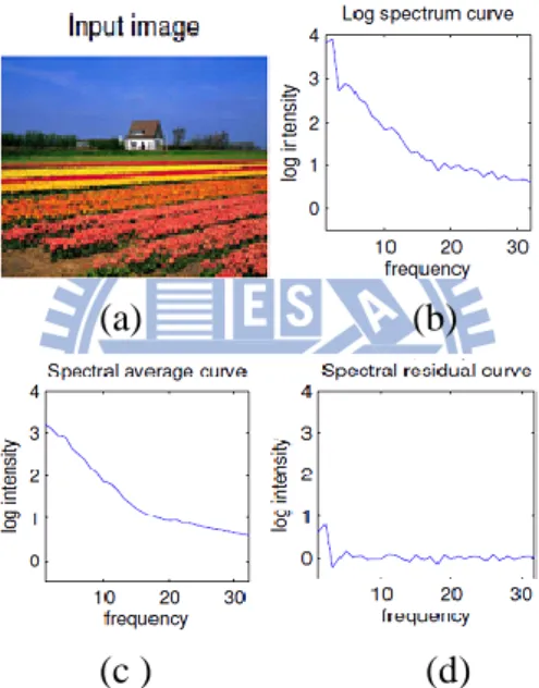
In spectrum domain, the method [7] applies the Spectral Residual (SR) and the simple Fourier Transform operation for object detection. In this approach, the authors obtain the spectral residual by subtracting the input image of log amplitude of spectrum with the reference of, as shown in Figure 2-12. The saliency map is then obtained by transforming the spectral residual back to the spatial domain.The saliency maps generated by [7] is shown in Figure 2-13(c). In spite of its simple operation, this SR method performed surprisingly well in detecting the saliency regions of many images.

(a) (b)

(c ) (d)

Figure 2-12 (a) Input image (b) corresponding log spectrum (c) reference (d) spectral residual

(a) (b) (c)

11

However, [8] points out the spectral residual of the log amplitude spectrum may be not essential to the calculation of the saliency map. On the contrary, only the phase spectrum plays the major role in detecting saliency regions. In [8], the saliency maps are generated only by transforming the phase spectrum of the image back to the spatial domain. The saliency map generated by [8] is shown in Figure 2-13(b).

Instead of transform domain approaches, [9] proposes the concept of the feature-pair which is the relation between the central point and its 8-connectivity neighbors as shown in Figure 2-14. In their approach, [9] first decompose input image into one intensity channel and two opponent-color channels. After that, [9] computes the feature-pairs of three channels and forms feature-pair distribution. A demonstration of intensity-pair distribution is shown in Figure 2-15. Finally, based the feature-pair distribution, [9] forms the 3-D histogram which is used for saliency analysis. The analysis result is then mapped back to the spatial domain to generate salient map. The saliency map generated by [9] is shown in Figure 2-15(b).

Figure 2-14 The main idea of feature-pair

12

(a) (b)

Figure 2-16 (a) Input image (b) saliency map by [9]

2.3 R

ECOGNITION

The shape is also an important feature of static waymarks. Authors in [3] apply the corner detector to recognize object shape, as shown in Figure 2-16. [4] uses the relation of boundary line (Figure 2-17) to determine the shape. The recent approach [5] uses the distance to borders (Dtbs) as the features of shape. The illustration of [5] is shown in Figure 2-18.

13

Figure 2-18 The relation of boundary line in [4]

(a) (b)

Figure 2-19 (a) The Dbts of triangle (b) the feature vectors of (a) by Dtbs [5]

After the shape recognition, we want to recognize the context inside the

shape. The current approach [2] applies the Histogram of Oriented Gradient descriptor (HOG) to obtain the features of the objects. In [2], they first divides the image into small connected regions, called cells. After that, each cell gathers a histogram of gradient directions for the pixels within the cell. Finally, these histograms of each cell are represented as the descriptor. For better accuracy, the measure of intensity across a larger region of the image, called a block, normalizes the histograms of each cell in

14

the block. This normalization enhances the robustness of the descriptor to lighting changes.

[10] proposes the concept of the Speeded Up Robust Features (SURF). The same as HOG, the input image is divided into many sub-regions. Each sub-region is analyzed by the Haar wavelet and the filter response in horizontal direction and vertical direction are denoted as d_x and d_y respectively. The wavelet responses

x

d and d_yare summed up over each sub-region as two feature vectors. In order to obtain extra information, they also extract the sum of the absolute values of the responses, d and_x d . Therefore, each sub-region has a four-dimensional descriptor _y

vectorv(

   

15

Chapter 3.

P

ROPOSED

M

ETHOD

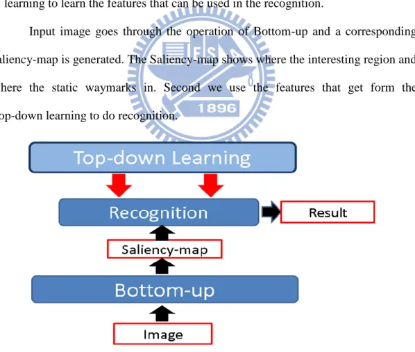
The goal of the system is to detect and recognize the static waymarks. The system includes two stages 1) Bottom-up, 2) Top-down learning.

1) Bottom-up: In this stage, the static waymarks in the image are fast identified. 2) Top-down learning: In this stage, we want to get the features of the static

waymarks which are useful for recognition. Here, we use the skills of machine learning to learn the features that can be used in the recognition.

Input image goes through the operation of Bottom-up and a corresponding saliency-map is generated. The Saliency-map shows where the interesting region and where the static waymarks in. Second we use the features that get form the Top-down learning to do recognition.

16

3.1. B

OTTOM

-U

P

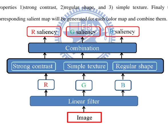
In Bottom-up, we want to fast identify the location of the static waymarks. Here, we find the physical properties to implement our Bottom-up algorithm. The static waymarks like fire hydra, bands have the following properties 1) strong contrast with respect to its surrounding regions 2) regular shape 3) simple texture. The three properties will be discussed in following section.

The flow chart of proposed Bottom-Up is illustrated in Figure 3-2. First the input image are decomposed into three color map R color, G color, and B color. Second these color map go through three operations based on three physical properties 1)strong contrast, 2)regular shape, and 3) simple texture. Finaly the corresponding salient map will be generated for each color map and combine them.

17

3.1.1. L

INEAR

F

ILTERING OF

I

MAGE

D

ATA

Because the color of the static waymarks is simple, similar to [6]‟s approach, we decompose an input image into a few feature vectors, including R color, G color, and B color, where r, g, and b denote the red, green, and blue components of the input image. For each color, negative values are set to zero.













3.1.2. S

TRONG

C

ONTRAST

In the Figure 3-3, we can notice the objects, (a) fire hydra, (b) blue band, and(c) unable parking band, have the strong contrast compare to the surroundings. This is because they are designed salient for the people. And in the top-down, we want to analyze the color of objects. Thus, we hope the algorithm that can not only show the strong contrast but also can do the analysis of color. Therefore we apply the feature-pair proposed by [9].

(a)fire hydra (b) blue band (c) unable parking band

18

For each of the R color, G color, and B color, we compute the feature-pair distribution as proposed in [9].

Take R component for example, we first analyze the relation between the central point and its 8-connectivity neighbors. In the Figure 3-4, we define the 8 neighbors of the point E and define the eight 2D coordinates (E,A) (E,B) (E,C) (E,D) (E,F) (E,G) (E,H) (E,I) as the R color-pairs. Here A, B….I is the R color value and the point A~I is the neighbor of E. Here we use the eight R color-pairs forming the R color-pair distribution.

Figure 3-4 The main idea of feature-pair

Figure 3-5 The feature-pair distribution

By using the R color-pairs of all the image pixels, we can obtain the R color-pair distribution as shown in Figure 3-6. Obviously, we can notice that the R color pairs in smooth regions will lie around the 45° line; whereas the R color pairs across edges will lie far from the 45°line.

Figure 3-6 shows an example of the R color-pair distribution of the fire hydrant image. It is clear that the road and grass are the major backgrounds of the image.

19

Therefore the R color-pairs of these two regions are two major clusters in the R color-pair distribution. On the other hand, the fire hydrant map to a smaller cluster in the top-right corner of the distribution. Moreover, the R color pairs over the road -grass boundary and the fire hydrant - grass boundary form four clusters (represented in green color) far away from the 45-degree line as shown in Figure 3-6.

In the R color-pair distribution, we can easily notice that the boundary between the fire hydrant and the grass show a stronger contrast than the road-grass boundary. Here we can conclude two facts that (1) the fire hydrant is “less common” than the road and grass; and (2) the fire hydrant has a stronger contrast compared to its background. We obtain the conclusion that the fire hydrant may attract the attention of most observers. We also form the G color-pair and the B color-pair distributions.

Figure 3-6 The example of R color-pair distribution

Similar to [10], we form a 3-D histogram by dividing the plane of feature-pair values into uniform cells and calculate the number of feature pairs in each cell. Most clusters lei around the diagonal in the 3-D histogram; the largest cluster corresponds to the background in the image; the foreground objects correspond to smaller clusters; and those clusters away from the diagonal correspond to the edge.

20

Figure 3-7 The 3-D histogram

Based on the 3-D histogram, a contrast-weighting algorithm is proposed to weigh the saliency degree of each cell around the diagonal. This weighting algorithm contains three main parts: the “edge weight” to gather the information that the off-diagonal cells provide, the “self weight” to determine whether a diagonal cell corresponds to a visually salient region, and the “foreground weight” to judge whether a diagonal cell corresponds to not the background.

The three parts are respectively base on three ideas 1) the stronger the edge is the more salient the objects are, 2) the smaller the size of objects is the more salient the objects are, and 3) the more different comparing to background is the more salient the objects are. Thus, we combine the three properties to the formulate

Edge weight

Color contrast weight Foreground weight Self weight

  Eq. 3-3

1) Edge weight

The Edge weigh is the edge that can give t how much contrast is. Edge weigh count is like Figure 3-8. The formulation is

2

_ ( , )

, {3 - _ }

Edge weight hist i j d

i j D histogram off the diagonal

  



Eq. 3-4

21

2) Self weight

The Self weight is the size of objects that can give t how much contrast is. The smaller the size of objects is the more salient the objects are. The formulation is

, { }

_ = ( , )

i j the histgram of the object

Self weight hist i j





Eq. 3-5

3) Foreground weight

The foreground weight is how different between objects and background. The more different comparing to background is the more salient the objects are. In the 3D histogram, the maximum of histogram on the diagonal is the background. And the foreground weight is how long to the maximum of histogram like Figure 3-9. The formulation is

F o r e g r o u n d_ w e i g h t Eq. 3-6 d

Figure 3-9 The 3-D histogram

22

3.1.3. R

EGULAR

S

HAPE

As we know, the static waymarks are different from the natural scene like trees, flowers. The main difference is the shape. In the Figure 3-10, we can find the shape of (a) fire hydra, (b) blue band, and (c) unable parking band is more regular than the surrounding.

(a) Fire hydra (b) blue band (c) unable parking band Figure 3-10 The example of the static waymarks

The regular shape means it is compounded of the straight line like horizontal, straight, oblique, and the circular line. Therefore the best way to implement the property is to detect the boundary. Here we find the filter banks have these properties. In the Figure 3-11, we use these filters to do convolution with the R color, B color, and G color. And the objects have the regular shape will response.

23

3.1.4. S

IMPLE

T

EXTURE

As we observe, the static waymarks are designed for easy identification. Thus they have to be designed differently compared to natural scenery. We notice that they are not complicated and have the simple texture compared the natural scenery.

In the paper [8], it mentions that if the signal is a pulse Figure 3-12 (a), the reconstructed signal based on the phase spectrum will have high response in location of input pulse.

(a) (b)

Figure 3-12 (a) Original signal(pulse) (b) Reconstruction result using phase [8] Then we find the specially designated objects also have the property. Look the Figure 3-13 (a). We find the blue band has simple texture and at the B channel (Blue) Figure 3-13 (b) we can notice it also has the property like pulse.

We find the specially designated object also like a pulse signal in nature image. Take Figure 3-13 (a) and (b) for example. Blue signboard in the image has simple texture. At B channel (Blue) it is the same as the situation depicted in Figure 3.12(a)

(a) (b) Figure 3-13 (a) Blue band (b) B color of blue band

Conversely, if the signal is not pulse but regular signal like sine Figure 3-14 (a), then we can find the result (b) has lower response. We think the natural scenery has

24

this property because it has more complex structure

(a) (b)

Figure 3-14 (a) Original signal(sine) (b) Reconstruction result using phase [8] The method of reconstruction result using phase is that

( , ) ( ( , )) f x y F I x y Eq. 3-7 ( , ) ( ( , )) p x y P f x y Eq. 3-8 ( , ) 2 ( , ) ( , ) * || [ i p x y ] || sM x y g x y F F e _{Eq. 3-9}

where F and F-1 denote the Fourier Transform and Inverse Fourier Transform, respectively. P(f) represents the phase spectrum of the image. g(x, y) is a 2D Gaussian filter. sM( x , y ) is reconstruction result using phase.

3.1.5. C

OMBINATION

Based on the three physical properties, we can obtain the three saliency maps which are normalized to one for each color map. The three saliency maps are combined and we apply the variance of them as the weighting (Eq.3-13). The R, G, and B saliency map are generated respectively by the Eq.3-10, 3-11, and 3-12.

1 2 3

_ _R _ _R _ _R _

R saliencyW R Contrast W R Shape W R Texture Eq.3-10

1 2 3

_ _G _ _G _ _G _

G saliencyW G Contrast W G Shape W G Texture Eq.3-11

1 2 3

_ _B _ _B _ _B _

B saliencyW B Contrast W B Shape W B Texture Eq.3-12











25

3.2. T

OP

-D

OWN

L

EARNING

In this section, we will discuss how we design a classifier for the recognition of the static waymarks. In order to achieve robustness to illumination, scale, and rotation, we chosen the color and shape as the features; then, a SVM classifier is trained based on the chosen features. Finally, we apply the Synthetic Minority Over-sampling Technique (Smote) algorithm to solve the problem of imbalanced data in the machine learning. The following sections are 1) color analysis and 2) shape analysis 3) SVM classifier 4) the algorithm of Smote

3.2.1. C

OLOR

A

NALYSIS

As we known, the RGB color space is sensitive to illumination change; therefore, we choose the HSI space as the candidate space for color analysis due to its robustness to illumination change.

In order to get color features, we obtain the histogram of hue and saturation and don‟t consider intensity. The example is shown in Figure 3-15(b) and (c).

(a) (b) (c)

26

3.2.2. S

HAPE

A

NALYSIS

Only color information is not enough for presenting the features of the static waymarks, hence the shape of the object is also taken into consideration. There are many methods to get the features of shape. However, in our system, we use the filter based approach for shape analysis because the shape of the static waymarks is composed of many different directional lines. Here we use the six directional lines to present the shape as shown in Figure 3.16. In order to be invariant to light change, we convolute the hue and saturation of the static waymarks with these filters as shown in Figure 3-17.

Figure 3-16 The six directional lines

Figure 3-17 The six directional filters

The challenge of the shape analysis is the rotation of the object. To take care of this issue, we use the descriptor in [12]. In this descriptor, we divide the patch into 24 regions as shown in Figure 3-18(a).The sum of value in each region constitutes the 24 dimensions features vectors. If the objects rotate, we have to adjust the feature vectors as shown in Figure3-18.

(a) (b) Figure 3-18 (a) Original (b) rotate

27

In order for rotation invariant, we have to adjust the features vector. Here we choose the method “maximum shift”. In the Figure 3-19, we divide the patch into 8 regions and get the sum of each region.

Figure 3-19 Maximum shift

If the maximum is region 5 in the Figure 3-20(a), we shift the regions 5, 13,

and 21 in the Figure 3-20 (b) to the top as shown in Figure 3-20 (c).

(a) (b)

(c)

Figure 3-20 (a) Find the maximum region (b) correspond region t (c) the result of shift

Although we apply “maximum shift”, we can‟t solve the problem of rotation. Example in Figure 3-21 demonstrates this problem. In Fig. 3.21, the object rotates in

28

(b). We can find the result of filter 1 in (a) is equal to the result of filter 2 in (a) if we use “maximum shift”. Therefore we also have to adjust the filers.

(a) (b)

Figure 3-21 (a) Find the maximum region (b) correspond region t (c) the result of shift

Here we use the “minimum shift” to adjust the filters. We calculate the sum of each result of filter and shift the result with minimum sum to the top as shown in Figure 3-22.

Figure 3-22 Adjust the result of filters

Through two shifting operation, our proposed method is invariant to rotation.

29

3.2.3. S

UPPORT

V

ECTOR

M

ACHINE

We apply the SVM classifier for data classification. In Figure 3-22, there are two classes: one is marked in blue and the other is marked in white. Here we want to find a hyper planethat separates two classes and H1, H2, and H3, are all possible hyper planes for data separation. The main idea of SVM classifier is to choose a hyper plane which can get the maximum margin of two set; therefore H3 is selected as the decision plane in SVM classification.

Figure 3-23 The three hyper planes to separate two sets

We have training data labeled as{ ,x_i y_i}, where 1... , { 1,1}, { d}.

i

i l y   x_i R In our proposed method, the vectors xiare color features and shape features, the

valuesy_i are “1” for one class and “-1” for the other class, d is the dimension of the vectorxi, and l is the number of training data. We find the hyper plane

{ , }w b that separates the two classes as shown in Figure 3-23. The vector w is

the normal to the hyper plane, b

w is the perpendicular distance from the hyper

30

Figure 3-24 Find the hyper plane

In order to separate the two set, the following constraints should satisfy:

( T ) 1 0

i i

y x w   b i Eq. 3-14

SVM classifier chooses the best hyper plane that has the maximum margin 2

w

by minimizing w in Figure 3-23. Minimizing the w is the same

minimizing 2

2

w _{. The problem can be summarized by minimizing}

2

w _{subject to}

the constraints Eq.3-14. Here we express the previous problem by the Lagrange multipliers as 2 , , 1 min{ [ ( ) 1]} 2 l i i b i c b  



The solution can be expressed by terms of linear combination of the training vectors

l i i i c  





31

3.2.4. S

YNTHETIC

M

INORITY

O

VER

-

SAMPLING

T

ECHNIQUE

(SMOTE)

The problem of our proposed method is imbalanced data. The number of the negative data is about 3000; however, the number of static waymarks data is about 40. The difference is about 60 times. In Figure 3-24(a), if the training data is balanced, the estimated decision boundary (solid balck line) will approximate the true boundary (solid red line) if there is few wrong data (black symbol „+‟). In contrary, if the training data is imbalanced (Figure 3-24(b)), the estimated decision boundary (solid black line) may be very far from the true boundary (solid red line) if there is few wrong data (black symbol „+‟).

(a) (b)

Figure 3-25 (a) Balanced data (b) imbalanced data

Thus, if the training data is imbalanced, we have to synthesize new data for the minority set. Here we apply SMOTE algorithm in [13].Synthetic samples are generated in the following way: Take the difference between the feature vector (sample) under consideration and its nearest neighbor. Multiply this difference by a random number between 0 and 1, and add it to the feature vector under consideration. This causes the selection of a random point along the line segment between two specific features. This approach effectively forces the decision region of the minority class to become more general. The following the pseudo-code for SMOTE in [13].

32

Algorithm SMOTE(T, N, k)

Input: Number of minority class samples T, Amount of SMOTE N%; Number of

nearest neighbors k

Output: (N/100)* T synthetic minority class samples

(*If N is less than 100%, randomize the minority class samples as only a random percent of them will be SMOTEd.*)

if N <100

then Randomize the T minority class samples T = (N/100) *T

N = 100

endif

N = (int)(N/100)

(* The amount of SMOTE is assumed to be in integral multiples of 100. *)

k = Number of nearest neighbors numattrs = Number of attributes

Sample[ ][ ]: array for original minority class samples

newindex: keeps a count of number of synthetic samples generated, initialized to 0 Synthetic[ ][ ]: array for synthetic samples(*Compute k nearest neighbors for

each minority class sample only. *)

for i ← 1 to T

Compute k nearest neighbors for i, and save the indices in the nnarray Endfor

Populate(N, i, nnarray) (*Function to generate the synthetic samples. *)

while N ~= 0

Choose a random number between 1 and k, call it nn. This step chooses one of the k nearest neighbors of i.

for attr ← 1 to numattrs

Compute: dif = Sample[nnarray[nn]][attr] − Sample[i][attr] Compute: gap = random number between 0 and 1

Synthetic[newindex][attr] = Sample[i][attr] + gap ∗ dif endfor

newindex++ N = N − 1

endwhile

return (* End of Populate. *) End of Pseudo-Code.

33

Chapter 4.

E

XPERIMENTAL

R

ESULTS

In this chapter, we will show and discuss our experimental results. In computer simulation, the proposed algorithm is coded in Matlab without code optimization, and is tested over a PC with Intel® Core™2 Duo CPU running at 3G Hz. The first experimental stage is to capture the video in the campus. Here we prepare three videos captured at different places for four different static waymarks. Figure 4-1 and 4-2 show the three places and the selected waymarks.

(a)

(b)

(c)

Figure 4-1 The overview of three places

34

In Table 4-1, for each static waymark, we randomly selected forty image patches in the video. The SOMTE algorithm was used to synthesize two hundred image patches as the positive training samples. On the other hand, three thousand image patches were extracted from the same video. The video was captured in the afternoon.

Table 4-1 Number of training images

Static waymarks The number selected SMOTE Blue signboard 40 200 Fire hydrant 40 200 Unable signboard 40 200 Parking signboard 40 200 Negative images 3000 X

In the Figure 4-3, we use the four colored bounding boxes to recognize four different static waymarks.

Figure 4-3 Use different colors bounding boxes for different static waymarks

The results of four static waymarks, with variations in rotation and scale, are shown in Figure 4-4 and 4-5.

35 (a)

(b)

(c)

Figure 4-4 Different scales of static waymarks in the afternoon

(a)

(b)

(c)

Figure 4-5 Static waymarks in the afternoon with rotation variations

Here we also apply our algorithm to the videos captured at noon and evening. The results are shown in Figure 4-6 and 4-7.

36 (a)

(b)

(c)

Figure 4-6 Static waymarks at noon with rotation variations

Figure 4-7 Static waymarks in the evening with rotation variations

Table 4-2 is the detection rate and false alarm for each static waymark at noon, afternoon, and evening. The number of testing image for each static waymark is about six hundreds. In Table 4-2, we find varying illumination is important effect at the detection rate. Moreover, if there are many objects similar to the static waymark, such as cripple signboard or parking signboard, the detection rate of the static waymark is lower than others.

37

Table 4-2 Detection rate and false alarm at different time for each static waymarks

Time Static waymarks Blue signboard Fire hydrant Cripple signboard Parking signboard Afternoon Detection rate 99.9% 99.9% 94.5% 93.5% False alarm (/1000 frames) 3 2 0 0 Noon Detection rate 99.9% 99.9% 90.5% 89.4% False alarm (/1000 frames) 1 4 15 0 Night Detection rate 94.2% 99.9% 92.1% 87.3% False alarm (/1000 frames) 14 9 1 0

In this thesis, we apply feature-pair, phase and directional filters for three physical properties 1) strong contrast, 2) simple texture, and 3) regular shape respectively. In Table 4-3, the three methods are use respectively for bottom-up detection.

Comparing to combining the three methods (Table 4-2), applying three methods respectively (Table 4-3) has little lower detection rate in the afternoon and much lower the detection rate at night, because of varying illumination. The result shows if we combine three methods we can obtain the good bottom-up detection and detection rate.

On other hand, in Table 4-4, we obtain the average computing time that includes detection and recognition by different bottom-up detection. The number of images is 2520 and the size of image is 360*240.

38

Table 4-3 Detection rate and false alarm for different bottom-up methods

Time Static waymarks Blue signboard Fire hydrant Cripple signboard Parking signboard Afternoon Detection rate 99.9% 99.9% 85.6% 93.4% False alarm (/1000 frames) 3 0 2 0 Night Detection rate 88.6% 99.9% 89% 82.3% False alarm (/1000 frames) 0 29 0 0 (a) Feature-pair Time Static waymarks Blue signboard Fire hydrant Cripple signboard Parking signboard Afternoon Detection rate 92.7% 99.9% 81.7% 90.4% False alarm (/1000 frames) 0 5 12 0 Night Detection rate 75.5%% 99.9% 79.2% 77.2% False alarm (/1000 frames) 22 15 0 0 (b) Phase Time Static waymarks Blue signboard Fire hydrant Cripple signboard Parking signboard Afternoon Detection rate 99.9% 99.1% 80.4% 88.7% False alarm (/1000 frames) 0 10 0 0 Night Detection rate 82.3%% 99.9% 70.6% 74.2% False alarm (/1000 frames) 3 13 0 0 (c) Directional filters

Table 4-4 Computing time for different bottom-up detection Bottom-up

methods

Combination Feature-pair Phase Directional filters

Time (second) (each image)

15.1s 16.9s 22.4s 30.8s

39

In Table 4-4, combining the three methods spends least time because it can make the static waymarks more salient and suppress the false alarm region.

We also consider our SVM classifier, which trained by the contain three places, using in other places. Figure 4-8 shows the overview of other three places.

(a) (b)

(c)

Figure 4-8 The overview of other three places

Table 4-5 shows the detection rate and false alarm for different places in the afternoon. The number of testing image is about 300 for each static waymarks.

Table 4-5 Detection rate and false alarm for three new places

Time Static waymarks Blue signboard Fire hydrant Cripple signboard Parking signboard Afternoon Detection rate 83.6% 99.2% 80.5% 86.7% False alarm (/1000 frames) 0 13 10 0

40

In Table 4-5, we can notice some static waymarks have high detection rate and some have low detection rate. In our opinion, if there are similar objects in the image the bottom-up detection has worse performance and we obtain the lower detection rate. Moreover, if the background is different the static waymarks the bottom-up detection has better performance and we can obtain high detection rate.

41

Chapter 5.

C

ONCLUSIONS

In this thesis, we propose a system of saliency-based detection and recognition for static waymarks with well performance. Based on three physical properties, the saliency detection can quickly identify the candidate regions in any newly captured video. Over the candidate regions, HSV color space and directional filter banks which are applied to analyze the color and shape respectively for the recognition of the pre-selected waymarks. These features are invariant to the lighting change, scale, rotation. Our system also considers the problem of different shapes and imbalanced training data. The result in chapter 4 shows the well detection rate under different condition such like at noon, in the afternoon, and at evening. We also obtain the lower detection rate for same static waymarks at different places.

42

R

EFERENCES

[1] Maldonado-Bascón S., Lafuente-Arroyo S., Gil-Jiménez P., Gómez-Moreno H., López-Ferreras F., “Road-Sign Detection and Recognition Based on Support Vector Machines”, IEEE Conference on Intelligent Transportation Systems, pp.

264 – 278.2007

[2] Y. Xie, L.-F. Liu, C.-H. Li, and Y.-Y. Qu, “Unifying visual saliency with hog feature learning for traffic sign detection,” IEEE Symposium on Intelligent

Vehicles, pp. 24 –29, June 2009.

[3] A. de la Escalera and L. Moreno, “Road traffic sign detection and classification.”

IEEE Trans. Indust. Electronics, 44:848–859, 1997.

[4] J. Miura, T. Kanda, and Y. Shirai, “An active vision system for real-time traffic signs recognition, IEEE Symposium on Intelligent Vehicles, pp. 52.57, Oct 2002. [5] S. Lafuente-Arroyo, P. Gil-Jiménez, R. Maldonado-Bascón, F. López-Ferreras,

and S. Maldonado-Bascón, “Traffic sign shape classification evaluation I: SVM using distance to borders,” in Proc. IEEE Intell. Veh. Symp., Las Vegas, NV, pp.

557–562 , Jun. 2005.

[6] L. Itti, C. Koch and E. Niebur, "A model of saliency-based visual attention for rapid scene analysis,” IEEE Transactions on Pattern Analysis and Machine Intelligence, vol. 20, pp. 1254-1259, 1998.

[7] X. Hou and L. Zhang, "Saliency detection: A spectral residual approach," IEEE

Conference on Computer Vision and Pattern Recognition, pp. 2280-2287, 2007.

[8] C. Guo, Q. Ma and L. Zhang, "Spatio-temporal saliency detection using phase spectrum of quaternion fourier transform," IEEE Conference on Computer Vision

and Pattern Recognition, pp. 2908-2915, 2008.

[9] Wen-Chung Huang, Sheng-Jyh Wang, and Cheng-Ho Hsin, "Visual Saliency Detection Based on Feature-Pair Distributions", in Proc. Computer Vision, Graphics, and Image Processing, Taiwan, 2009

[10] H. Bay, T. Tuytelaars, and L. Van Gool. “SURF: Speeded Up Robust Features”,

Proceedings of the ninth European Conference on Computer Vision, May 2006.

[11] M. Varma and A. Zisserman. A statistical approach to material classification using image patch exemplars. PAMI, 31(11):2032–2047, November 2009.

[12] S. Belongie, J. Malik, and J. Puzicha, “Shape Matching and Object Recognition Using Shape Contexts,” IEEE Trans.Pattern Analysis and Machine Intelligence, 24(4):509–522, 2002.

43