台灣權證市場對股票市場之影響及投資人情緒 - 政大學術集成

全文

(1)國立政治大學財務管理研究所. 碩士論文. 治政台灣權證市場對股票市場之影響及投資人情緒大立 ‧ 國. 學. The Impact of the Warrant Market on the Stock Market and. ‧. Investor Sentiment: Taiwan Evidence. n. er. io. sit. y. Nat. al. Ch. engchi. i n U. 指導教授：李志宏博士研究生：陳裕軒. 中華民國一百年七月. v.

(2) Abstract This paper examines the relation between the stock liquidity and warrants expiration in different extent of investor sentiment which is represented by VIX in Taiwan. We study the effect of trading consolidation by examining the response of liquidity and stock prices to the exercise of deep in-the-money call warrants. In general, the results indicate that the stock liquidity is improved apparently by market consolidation since warrants expired when investor sentiment is relatively low. On the other hand, the effect is insignificant when VIX is relatively high.. 政治大. Further, the price increase is positively related to post-exercise improvement in the. 立. stock liquidity when VIX is relatively low. While VIX rises, the relation gets feeble. ‧ 國. 學. gradually. This phenomenon might be due to investors’ buying behavior such as arbitrage or hedge trading varying with different kinds of market situation.. ‧. n. al. er. io. sit. y. Nat. Key words: warrant, stock, liquidity, consolidation, investor sentiment.. Ch. engchi. I. i n U. v.

(3) Contents Abstract .................................................................................................................... I I.. Introduction ..................................................................................................... 1. II.. Data ............................................................................................................... 3. III.. Methodology ................................................................................................ 4 A.. Trading Volume ....................................................................................... 4. B.. Implicit Spread, Turnover, and Market Depth ..................................... 4. C.. The Relation of Liquidity Changes to Fragmentation ......................... 5. D.. The Effect of Warrant Exercise on Stock Values.................................. 6. E.. Investor Sentiment .................................................................................. 7. ‧ 國. 學. IV.. 立. 政治大. Empirical Results ........................................................................................ 8 Hypothesis ................................................................................................ 8. B.. The Analysis of Abnormal Returns ....................................................... 9. C.. Liquidity Change and Cumulative Abnormal Returns ..................... 15. D.. Investor Sentiment ................................................................................ 21. E.. The Change in Investor Sentiment ...................................................... 28. ‧. A.. n. er. io. sit. y. Nat. al. V.. Ch. engchi. i n U. v. Conclusions and Discussion .......................................................................... 40. References .............................................................................................................. 42 Appendix ................................................................................................................ 44. II.

(4) Table Contents Table 1 The Structure of all the Warrants Issued in 2006-2010 at the First Trading Dates ........................................................................ 3 Table 2 The Abnormal Returns of Stocks around the Issued Dates of All Warrants .................................................................................... 9 Table 3 The Abnormal Returns of Stocks around the First Trading Dates of All Warrants .................................................................... 10 Table 4 The Abnormal Returns of Stocks around the Expiration Dates of All Warrants .................................................................... 11 Table 5 The Abnormal Returns of Stocks During the Issued Dates of All Warrants in the Period of High VIX ..................................... 11. 政治大 Dates of All Warrants in the Period of High VIX....................... 12 立 Table 7 The Abnormal Returns of Stocks During the Expiration Table 6 The Abnormal Returns of Stocks During the First Trading. ‧ 國. 學. Dates of All Warrants in the Period of High VIX....................... 12. Table 8 The Abnormal Returns of Stocks During the Issued Dates of. ‧. All Warrants in the Period of Low VIX ...................................... 13. Table 9 The Abnormal Returns of Stocks During the First Trading. y. Nat. sit. Dates of All Warrants in the Period of Low VIX........................ 13. er. io. Table 10 The Abnormal Returns of Stocks During the Expiration. al. v i n Table 11 The Abnormal During the Expiration C h Returns of Stocks U i e h n g c Warrants ..................................14 Dates of All Deep In-the-money n. Dates of All Warrants in the Period of Low VIX........................ 14. Table 12 The Abnormal Returns of Stocks During the Expiration Dates of All Non-Deep In-the-money Warrants ......................... 15 Table 13 Changes in The stock liquidity following the warrant Exercise .......................................................................................... 17 Table 14 Determinants of the Cumulative Abnormal Return (CAR) on the Expiration of All Deep-in-the-Money Warrants ............. 19 Table 15 Changes in The stock liquidity following the warrant Exercise in the Period of High VIX ............................................. 22 Table 16 Determinants of the Cumulative Abnormal Return (CAR) on the Expiration of All Deep-in-the-Money Warrants in the. III.

(5) Period of High VIX ....................................................................... 24 Table 17 Changes in The stock liquidity following the warrant Exercise in the Period of Low VIX .............................................. 25 Table 18 Determinants of the Cumulative Abnormal Return (CAR) on the Expiration of All Deep-in-the-Money Warrants in the Period of Low VIX ........................................................................ 27 Table 19 Changes in The stock liquidity following the warrant Exercise from the Period of Low VIX to Low VIX .................... 29 Table 20 Determinants of the Cumulative Abnormal Return (CAR) on the Expiration of All Deep-in-the-Money Warrants from the Period of Low VIX to Low VIX ................................................... 30. 治政大to High VIX ...................32 Exercise from the Period of Low VIX 立 Table 22 Determinants of the Cumulative Abnormal Return (CAR). Table 21 Changes in The stock liquidity following the warrant. ‧ 國. 學. on the Expiration of All Deep-in-the-Money Warrants from the Period of Low VIX to High VIX .................................................. 33. ‧. Table 23 Changes in The stock liquidity following the warrant Exercise from the Period of High VIX to Low VIX ................... 35. y. Nat. sit. Table 24 Determinants of the Cumulative Abnormal Return (CAR). al. er. io. on the Expiration of All Deep-in-the-Money Warrants from the. n. Period of High VIX to Low VIX .................................................. 36. Ch. i n U. v. Table 25 Changes in The stock liquidity following the warrant. engchi. Exercise from the Period of High VIX to High VIX .................. 37 Table 26 Determinants of the Cumulative Abnormal Return (CAR) on the Expiration of All Deep-in-the-Money Warrants from the Period of High VIX to High VIX ................................................. 39 Table A 1 Securities Trading Value Percentage by Type of Investors ......................................................................................................... 44. IV.

(6) I.. Introduction According to many previous literatures, for examples, Aitken and Segara (2005),. Amihud, Lauterbach, and Mendelson (2003), Chan and Wei (2001), we have assured that warrants and stocks have somehow correlation in price, liquidity and volatility. If they truly exist some strong correlation between warrants and stocks, we may have arbitrage opportunities. Chan and Wei (2001) contend that the prices of underlying stocks peak on the first day after the warrant announcement and stay stable. Thereafter, the information effect. 政治大 according to the study of Aitken and Segara (2005), they find that there are significantly 立. associated with the warrant issuance appears to be weak and does not last long. However,. ‧ 國. 學. negative abnormal returns (ARs) of underlying stocks on both the announcement and the listing dates of derivative warrants. Since the different countries have different types of. ‧. investors and behaviors, we want to figure out whether the abnormal returns would exist. sit. y. Nat. in different kinds of market situation or not.. io. er. In this paper, we will observe how stock prices, liquidity, volatility move on the. al. certain of the key days. For example, announcement dates, first trading dates, and. n. v i n C hthe previous literatures, expiration dates of warrants. From e n g c h i U most of them focused on only one event. Therefore we want to dig comprehensively. We chose Taiwan as our target market－the world’s 12th largest financial market (Barber, Lee, Liu, and Odean (2009)). In Taiwan, nearly 70% of investors are individuals (showed in Appendix Table A1). The investor structure is quite different to other countries, such as the United States. The warrant market has become popular in Taiwan in recent years. According to the increasing trading volume of warrants, we think that the correlation between the warrant market and the stock market would be stronger. Our study examines all the call warrants exercised on TWSE (Taiwan Stock. 1.

(7) Exchange) and TWO (Taiwan OTC Exchange) during 2006-2010. Amihud, Lauterbach, and Mendelson (2003) find that liquidity and stock prices both increase significantly at warrant expiration while those warrants are deep in the money prior to the expiration day. According to their study, we focus on the warrants which are deep in-the-money. Whereas their exercise is quite certain, it suggests that we can eliminate time value and information cost inside the warrants. In addition, we want to know the correlation between investor sentiment and the stock market. Would investor sentiment affect the change of the stock liquidity after. 治政 has larger effects on securities whose valuations are 大 highly subjective and difficult to 立 warrants expired? Baker and Wurgler (2006) contend that a wave of investor sentiment. arbitrage. We want to see whether investor sentiment would affect the ARs of underlying. ‧ 國. 學. stocks and the liquidity improvement or not. Is there any chance we could arbitrage. ‧. during the different degrees of investor sentiment? We use the VIX 1 of Taiwan, which is. sit. y. Nat. gathered statistics by Taiwan Futures Exchange, to distinguish how volatile the market is. io. n. al. er. and use it as a proxy of investor sentiment.. Ch. engchi. 1. i n U. v. VIX: Taiwan Futures Exchange used the same concept and calculating formula from Chicago Board Options Exchange Volatility Index. It is the implied volatility of option market representing the expected volatility in the following 30 days.. 2.

(8) II.. Data We collected all warrants and stocks daily data from Taiwan Economic Journal Co.,. Ltd (TEJ) data base. The sample period is from January, 2006 to June, 2010. TWSE had changed the trading mechanism of warrants since June 28th, 2010, so we only collected our warrants data before the day of changing the trading mechanism to exclude that factor. Our sample consists of all the warrants that were exercised on TWSE and TWO over the period 2006-2010. There are 28078 warrants issued in 2006-2010 (we could see the. 政治大 consolidation of two identical securities into one, so we have to confine our study to 立. structure of all warrants showed in Table 1). Nevertheless, we want to consider the. ‧ 國. 學. those warrants that are practically substitutes of the stock. In hence, we obtain that our choice criterion is satisfied for S/X≧1.10, where S is the stock price and X is the. ‧. warrant exercise price. We thus set the cutoff at S/X＝1.10, that is, we exclude those. Nat. sit. y. warrants that are S/X＜1.10 three days before expiration from our data. In addition, to. n. al. er. io. simply our samples, we only use the data of call warrants. And the underlying stocks are. i n U. v. all individual stocks. There are 3549 warrants that qualify for our research.. Ch. engchi Table 1. The Structure of all the Warrants Issued in 2006-2010 at the First Trading Dates Price Percentage. In-the-Money. At-the-Money. Out-of-Money. 6.01%. 0.21%. 93.78%. 28078. Numbers of sample. In-the-Money represents that S/X＞1 on call warrants and S/X＜1 on put warrants. At-the-Money represents that S/X＝1 on both calls and puts. Out-of-Money represents that S/X＜1 on calls and S/X＞1 on puts. The sample comprises 28078 warrants over the period 2006-2010.. 3.

(9) III.. Methodology. A. Trading Volume The measures of liquidity are based on Amihud, Lauterbach, and Mendelson (2003). First, we use the change of the stock’s trading volume to measure liquidity. We calculate the change in the relative trading volume in the stock as follows. Let DVOLj denote the change in the trading volume of stock j relative to the market volume, (1) 𝐷𝑉𝑂𝐿𝑗 = 𝑙𝑜𝑔�𝑉𝑂𝐿𝑗𝐴 ∕ 𝑉𝑂𝐿𝐴𝑚 � − 𝑙𝑜𝑔�𝑉𝑂𝐿𝑗𝐵 ∕ 𝑉𝑂𝐿𝐵𝑚 �,. 政治大 and the market, respectively. 立 A indicates the period of 30 trading days following the. where VOL is the average daily volume (in monetary units) and j and m indicate stock j. ‧ 國. 學. expiration window, (days ＋1 to ＋30), B indicates the period of 30 trading days before the expiration window (days －30 to －1), and the expiration window consists of the. ‧. one trading day straddling the expiration day.. er. io. sit. y. Nat. B. Implicit Spread, Turnover, and Market Depth. al. v i n C h using the autocovariance bid-ask spread which can be calculated of stock returns, engchi U n. The second measure of liquidity is based on Roll (1984), who shows that the implicit. COVj＝COV (Rj,t, Rj,t－1), as (2) 𝑆𝑃𝑅𝐸𝐴𝐷𝑗 = 2 ∙ �−𝐶𝑂𝑉𝑗 . We calculate the COVj of each stock j from daily returns over 30 trading days before (B) and 30 trading days after (A) the warrant expiration window. The change in the bid-ask spread, (3) 𝐷𝑆𝑃𝐷𝑗 = 𝑆𝑃𝑅𝐸𝐴𝐷𝑗𝐴 − 𝑆𝑃𝑅𝐸𝐴𝐷𝑗𝐵 , 4.

(10) can be used as an estimate of the change in liquidity. The third measure of liquidity is the turnover rate of trading volume which can be calculated as following equation, 𝑇𝑟𝑎𝑑𝑖𝑛𝑔 𝑉𝑜𝑙𝑢𝑚𝑒. 𝑗 (4) 𝑇𝑅𝑄𝑗 = 𝑆h𝑎𝑟𝑒𝑠 𝑂𝑢𝑡𝑠𝑡𝑎𝑛𝑑𝑖𝑛𝑔 . 𝑗. We calculate the TRQj of each stock j by using the same window on COVj. Then we define DTRQ as the following equation, 𝑇𝑅𝑄𝐴. (5) 𝐷𝑇𝑅𝑄𝑗 = 𝑙𝑜𝑔 �𝑇𝑅𝑄𝑗𝐵 �, 𝑗. 政治大. 立. which represents the change in the turnover rate of trading volume.. ‧ 國. 學. The fourth measure of liquidity is the standard deviation of returns of closed prices. ‧. 𝑠𝑡𝑑.. n. which represents the change in the market depth.. Ch. 𝐵. er. io. al. 𝐴. sit. Nat. 𝑠𝑡𝑑.. (6) 𝐷𝑠𝑡𝑑𝑗 = 𝑙𝑜𝑔 �𝑇𝑟𝑎𝑑𝑖𝑛𝑔 𝑉𝑜𝑙𝑢𝑚𝑒� − 𝑙𝑜𝑔 �𝑇𝑟𝑎𝑑𝑖𝑛𝑔 𝑉𝑜𝑙𝑢𝑚𝑒� ,. y. which is divided by the daily trading volume of stock j. We define it as below,. engchi. i n U. v. C. The Relation of Liquidity Changes to Fragmentation Now we use the following regressions to test whether the consolidation of trading could increase liquidity by the warrant exercise. If so, the increase in liquidity should be positively related to the degree of fragmentation before the warrant expiration. (7) 𝐷𝐿𝐼𝑄𝑈𝐼𝐷𝐼𝑇𝑌𝑗 = 𝛾0 + 𝛾1𝑉𝑂𝐿𝑅𝑊𝑆𝑗 + 𝑢𝑗 VOLRWSj denotes the ratio of the average daily trading volume of warrants to the average daily trading volume of the underlying stocks in the period of 30 trading days. 5.

(11) (days －30 to －1) before the warrants expiration. For DLIQUIDITYj, we use DVOLj, DSPDj, DTRQj, and Dstdj, the measures of the change in the stock liquidity at the warrant expiration.. D. The Effect of Warrant Exercise on Stock Values As we explain in the introduction, we want to see how the exercise of warrant affects stock prices. First, we calculate the abnormal returns 2, (8) 𝐴𝑅𝑗𝑡 = 𝑅𝑗𝑡 − 𝑅𝑀𝑡 ,. 政治大. where Rjt is the return on stock j on day t, and RMt is the return of market index on day t.. 立. Then we calculate the two-day (days －1 and 0) cumulative abnormal returns,. ‧ 國. 學 ‧. (9) 𝐶𝐴𝑅𝑗 = 𝐴𝑅𝑗,−1 + 𝐴𝑅𝑗,0 .. After we define CARj, we want to figure out whether CARj is an increasing function. y. Nat. al. er. io. sit. of the liquidity benefits from consolidation. We use the following regression,. n. (10) 𝐶𝐴𝑅𝑗 = 𝛿0 + 𝛿2 𝐷𝐿𝐼𝑄𝑈𝐼𝐷𝐼𝑇𝑌𝑗 + 𝜈𝑗 .. Ch. engchi. i n U. v. DLIQUIDITYj＝DVOLj, DCOVj, DTRQj, or Dstdj, or two of them. Then considering the change in trading volume of the firm’s equity claims in excess of the increase in the number of shares following the warrant exercise, (11) 𝐷𝑉𝑂𝐿𝑅𝐴𝑇𝑗 = 𝐷𝑉𝑂𝐿𝑗 − 𝑙𝑜𝑔�1 + 𝑅𝐴𝑇𝑊𝑆𝑗 �. DVOLRATj is the difference between the relative change in the stock’s trading volume, 2. We could see Brown and Warner (1980, 1985) on this method of calculating the abnormal return. In our case, it is inappropriate to employ the conventional market model methodology and estimate the market model parameters in the period before the expiration. Because in some cases a warrant enters our sample of deep in-the-money warrants after a rise in the price of the underlying stock before the warrant expiration.. 6.

(12) DVOLj, and RATWSj, the relative increase indirectly in the number of shares of stock that results from the warrant exercise (despite investors can choose to receive stocks or cash when warrants expire). RATWSj is the ratio of the number of warrants to the number of shares of stock outstanding.. E. Investor Sentiment We use the VIX of Taiwan which is calculated by Taiwan Futures Exchange as a proxy of investor sentiment. The VIX of Taiwan is used starting from December, 2006. To match VIX, we have to give up parts of our samples are before December, 2006.. 政治大. Following the criteria used by Bliss and Panigirtzoglou (2004), we use the mean of VIX. 立. in the all sample period to determinate whether the VIX is relatively high or low.. ‧ 國. 學. The mean value of VIX in the all sample period is 26.85. We calculate the mean value of VIX during the period of 30 trading days before and after the expiration dates. ‧. following the window of (－30, －1) and (＋1, ＋30), respectively. If the mean of VIX. y. Nat. io. sit. is higher than 26.85, then we define it as the period of high VIX. Corresponsively, if the. n. al. er. mean of VIX is lower than 26.85, it represents the period of low VIX.. Ch. engchi. 7. i n U. v.

(13) IV.. Empirical Results. A. Hypothesis Our main test is whether stock prices are affected by the trading consolidation or not. Given that the warrants exercise on the expiration dates have no information content (we include only warrants that are deep in-the-money prior to expiration), our null hypothesis is that the ARs on the stock is zero. Against the null, the first alternative hypothesis is:. 政治大. H1. Stock prices should rise if consolidation of trading is beneficial.. 立. However, it could be argued that warrants offer investors additional tools to diversify. ‧ 國. 學. their investment portfolios, upon warrants exercise, might reduce investors’ incentive and interest to invest in the stocks. Therefore, we consider another alternative. ‧. hypothesis:. sit. y. Nat. io. er. H2. Stocks prices should fall because of the elimination of investment tools of diversifying afforded by warrants.. n. al. Ch. engchi. i n U. v. In fact, the both effects may be present. The results will show us which effect is stronger. Hypothesis H1 posits that the rise in stock prices is due to the increase in the stock liquidity upon the consolidation of trading after the warrants expiration. We exam this hypothesis by testing the relation between CAR and variables that reflect the liquidity benefits of trading consolidation. Our hypothesis is: H3. CAR is an increasing function of liquidity benefits from consolidation of trading following the warrants expiration.. 8.

(14) B. The Analysis of Abnormal Returns As mentioned in the part of introduction, first we want to see the abnormal returns (ARs) of stocks around the issued dates, the first trading dates, and the expiration dates of all warrants. We could see the statistic results in Table 2, 3 and 4. In Table 2, the results show that almost all the means of daily ARs of stocks around the issued dates of all warrants are significantly positive. These results are contrary to the paper written by 張啟容 (1998), which discovered that there are negative ARs on the issued dates significantly. The paper uses the data in the sample period from 1997 to. 政治大 convey somehow a kind of negative signal to investors. However, in our sample period, 立 1998 in Taiwan, and the author considered that the events of issuing warrants would. ‧ 國. 學. the phenomenon does not exist anymore. Conrad (1989) finds that options would have positive price effects on stocks beginning approximately three days before introduction.. ‧. And the effects are significantly until the day after issuing. Although warrants are not. sit. y. Nat. exactly like options, the results from Conrad (1989) are somewhat consistent with ours.. n. al. er. io. We think that issuers might buy portions of stocks to build their positions for hedge. v. before they issue the warrants. Therefore the behavior of inventory buildup may lead the. Ch. engchi. i n U. stock prices rising. This explanation is consistent with the study from Chan and Wei (2001). Table 2 The Abnormal Returns of Stocks around the Issued Dates of All Warrants t-3. t-2. t-1. t. t+1. Mean. 0.2790***. 0.2894***. 0.0850***. 0.0874***. 0.0682***. 0.0248. 0.0313*. Std.. 2.5503. 2.5101. 2.3336. 2.2985. 2.2936. 2.2453. 2.2504. t-value. 13.19. 13.90. 4.39. 4.58. 3.58. 1.33. 1.68. N. t+2. t+3. 14528. Day t is the issued dates of warrants. The abnormal returns (ARs) of stocks are the daily returns of underlying stocks minus the daily market returns. The sample comprises 14528 warrants over the period 2006-2010. ***, **, and * indicate significant level 1%, 5%, and 10%, respectively.. 9.

(15) In Table 3, it shows the results of the means of the ARs of stocks around the first trading dates of all warrants are almost significantly positive. On average, issuers would sell out their issuing positions in the first three days after the warrants listing (王佩甄 (2000)). However, there is no strong evidence to explain the ARs of stocks after the first trading dates of warrants. We infer a possible explanation is that since most of warrants are issued out-of-money (showed in Table 1), if issuers want to sell out their issuing warrants as soon as possible, they might somewhat play a role of market makers in the stock market to stimulate the stock prices to go up.. 政 Table治 3 大 The Abnormal Returns 立 of Stocks around the First Trading Dates of All Warrants. ‧ 國. t-2. t-1. t. t+1. t+2. t+3. 學. t-3. 0.0225. 0.0340*. 0.0878***. 0.1348***. 0.1850***. 0.1674***. 0.1945***. Std.. 2.2778. 2.2349. 2.2599. 2.2508. 2.2879. 2.2986. 2.2617. t-value. 1.19. 1.83. 4.68. 7.22. 9.74. 8.78. 10.36. y. 14521. Nat. N. ‧. Mean. sit. n. al. er. io. Day t is the first trading dates of warrants. The abnormal returns (ARs) of stocks are the daily returns of underlying stocks minus the daily market returns. The sample comprises 14521 warrants over the period 2006-2010. ***, **, and * indicate significant level 1%, 5%, and 10%, respectively.. i n U. v. In Table 4, we could see that the days before expiration dates and the event dates. Ch. engchi. have negative ARs of stocks. But the days after expiration dates have significantly positive ARs of stocks. We infer that investors might prefer to invest in the same equity claim. Since the warrants expired, investors have to rebalance their positions. The results could be explained that stock prices are improved by trading consolidation. We will discuss the relation between prices, liquidity, and trading consolidation in detail in the following section.. 10.

(16) Table 4 The Abnormal Returns of Stocks around the Expiration Dates of All Warrants t-3. t-2. t-1. t. t+1. Mean. 0.0662***. 0.0821***. Std.. 2.1241. t-value. 3.70. -0.0003. -0.0327*. 2.1791. 2.1095. 4.47. 0.02. N. t+2. t+3. 0.0703***. -0.0026. -0.0112. 2.1442. 2.0433. 2.0965. 2.0704. 1.81. 4.08. 0.15. 0.64. 14102. Day t is the expiration dates of warrants. The abnormal returns (ARs) of stocks are the daily returns of underlying stocks minus the daily market returns. The sample comprises 14102 warrants over the period 2006-2010. ***, **, and * indicate significant level 1%, 5%, and 10%, respectively.. Further, we want to see if different level of investor sentiment would affect the ARs. 政治大 stocks before t+2 are all as significantly positive as the results in Table 2. There is no 立. of stocks or not. In Table 5, we could see that in the period of high VIX, the ARs of. ‧ 國. 學. apparent difference when investor sentiment is relatively high. Table 5. ‧. The Abnormal Returns of Stocks During the Issued Dates of All Warrants in the. io. Mean. 0.2729***. Std.. 2.8675. 2.7640. t-value. 7.33. 8.14. 0.2919***. al. n. N. t-1. y. sit. t-2. t. t+1. 0.0666*. 0.1023***. 0.0936***. 2.6204. 2.6161. C1.96 h e n g c3.01h i. er. Nat. t-3. Period of High VIX. 2.6087 iv n U 2.76. t+2. t+3. 0.0348. -0.0385. 2.5563. 2.5529. 1.05. 1.16. 5935. Day t is the issued dates of warrants. The abnormal returns (ARs) of stocks are the daily returns of underlying stocks minus the daily market returns. The sample comprises 5935 warrants in the period of high VIX (we calculate the mean value of VIX during the period of 30 trading days before and after the issued dates following the window of (－30, ＋30)) exercise over 2006-2010. ***, **, and * indicate significant level 1%, 5%, and 10%, respectively.. Next, we could see the ARs of stocks after t-1 in Table 6 are all as significantly positive as the results in Table 3. Apparently, the ARs of stocks after the first trading dates would not be significantly affected by investor sentiment.. 11.

(17) Table 6 The Abnormal Returns of Stocks During the First Trading Dates of All Warrants in the Period of High VIX t-3. t-2. t-1. t. t+1. t+2. t+3. Mean. -0.0325. -0.0407. 0.0423. 0.0680**. 0.1873***. 0.1317***. 0.2030***. Std.. 2.5696. 2.5313. 2.5539. 2.5796. 2.5830. 2.5998. 2.5245. t-value. 0.97. 1.24. 1.27. 2.03. 5.58. 3.90. 6.19. N. 5924. Day t is the first trading dates of warrants. The abnormal returns (ARs) of stocks are the daily returns of underlying stocks minus the daily market returns. The sample comprises 5924 warrants in the period of high VIX (we calculate the mean value of VIX during the period of 30 trading days before and after the first trading dates following the window of (－30, ＋30)) exercise over 2006-2010. ***, **, and * indicate significant level 1%, 5%, and 10%, respectively.. 政治大. In Table 7, we could see the ARs of stocks on the day t are different from the results. 立. in Table 4. So in the period of high VIX, the ARs of stocks on the expiration dates are. ‧ 國. 學. not significantly negative.. ‧. Table 7. n. al. t-1. Mean. 0.1493***. 0.1407***. Std.. 2.5419. 2.5865. t-value. 3.78. 3.50. t. 0.0297. 0.0095. C 2.5210 h e n g c2.5370 hi 0.76 0.24. N. t+1. er. t-2. sit. the Period of High VIX. io. t-3. y. Nat. The Abnormal Returns of Stocks During the Expiration Dates of All Warrants in. 0.1310*** iv n U 2.4491 3.44. t+2. t+3. 0.1020***. 0.0565. 2.5355. 2.4600. 2.59. 1.48. 4133. Day t is the expiration dates of warrants. The abnormal returns (ARs) of stocks are the daily returns of underlying stocks minus the daily market returns. The sample comprises 4133 warrants in the period of high VIX (we calculate the mean value of VIX during the period of 30 trading days before and after the expiration dates following the window of (－30, ＋30)) exercise over 2006-2010. ***, **, and * indicate significant level 1%, 5%, and 10%, respectively.. In Table 8, we could see that the ARs of stocks during the issued dates before t+2 are all as significantly positive as the results in Table 2 and Table 5. It suggests no matter in what levels of VIX, the existence of ARs of stocks is lasting.. 12.

(18) Table 8 The Abnormal Returns of Stocks During the Issued Dates of All Warrants in the Period of Low VIX t-3. t-2. t-1. t. t+1. Mean. 0.2832***. 0.2877***. 0.0977***. 0.0771***. 0.0507**. 0.0179. 0.0796***. Std.. 2.3061. 2.3188. 2.1130. 2.0506. 2.0478. 2.0026. 2.0139. t-value. 11.39. 11.50. 4.29. 3.48. 2.29. 0.83. 3.66. N. t+2. t+3. 8593. Day t is the issued dates of warrants. The abnormal returns (ARs) of stocks are the daily returns of underlying stocks minus the daily market returns. The sample comprises 8593 warrants in the period of low VIX (we calculate the mean value of VIX during the period of 30 trading days before and after the issued dates following the window of (－30, ＋30)) exercise over 2006-2010. ***, **, and * indicate significant level 1%, 5%, and 10%, respectively.. 政治大. Then we could see the results showed in Table 9, comparing with Table 3 and Table. 立. 6, the ARs of stocks are all as significantly positive as the results above. It proves again. ‧ 國. 學. that the investor sentiment did not visibly affect the ARs of stocks during the first trading. ‧. dates of warrants.. y. sit. Nat. Table 9. io. n. al. the Period of Low VIX. Ch. t-3. t-2. t-1. Mean. 0.0604***. 0.0854***. Std.. 2.0521. 2.0033. 2.0324. t-value. 2.73. 3.95. 5.44. t. er. The Abnormal Returns of Stocks During the First Trading Dates of All Warrants in. v it+1 n U. t+2. t+3. 0.1834***. 0.1920***. 0.1887***. 1.9918. 2.0602. 2.0655. 2.0614. 8.42. 8.25. 8.62. 8.49. e n g0.1808*** chi. 0.1192***. N. 8597. Day t is the first trading dates of warrants. The abnormal returns (ARs) of stocks are the daily returns of underlying stocks minus the daily market returns. The sample comprises 8597 warrants in the period of low VIX (we calculate the mean value of VIX during the period of 30 trading days before and after the first trading dates following the window of (－30, ＋30)) exercise over 2006-2010. ***, **, and * indicate significant level 1%, 5%, and 10%, respectively.. In Table 10, we could see that the ARs of stocks are almost as same as the results in Table 4. According to our results, we could infer that the effects of investor sentiment play a role in the ARs of stocks during the expiration dates of warrants. As we exam the. 13.

(19) variances of the ARs of stocks during the issued dates and the first trading dates in different levels of VIX, there is no visibly change among our statistic results. Table 10 The Abnormal Returns of Stocks During the Expiration Dates of All Warrants in the Period of Low VIX t-3. t-2. t-1. t. t+1. t+2. t+3. Mean. 0.0318*. 0.0578***. -0.0128. -0.0502**. 0.0451**. -0.0459**. -0.0393**. Std.. 1.9236. 1.9855. 1.9132. 1.9582. 1.8486. 1.8832. 1.8849. t-value. 1.65. 2.90. 0.67. 2.56. 2.44. 2.43. 2.08. N. 9969. 政治大. Day t is the expiration dates of warrants. The abnormal returns (ARs) of stocks are the daily returns of underlying stocks minus the daily market returns. The sample comprises 9969 warrants in the period of low VIX (we calculate the mean value of VIX during the period of 30 trading days before and after the expiration dates following the window of (－30, ＋30)) exercise over 2006-2010. ***, **, and * indicate significant level 1%, 5%, and 10%, respectively.. 立. ‧ 國. 學. In this paper, we mainly focus on the warrants which are deep in-the-money. The. ‧. exercise of those type of warrants is quite certain, it suggests that we can eliminate time. sit. y. Nat. value and information cost inside the warrants. In Table 11, comparing with the results in. io. al. er. Table 4, the ARs of stocks on the expiration dates of deep in-the-money warrants are. n. more significantly negative than the results of all warrants.. Ch. e nTable g c11h i. i n U. v. The Abnormal Returns of Stocks During the Expiration Dates of All Deep In-the-money Warrants t-3. t-2. t-1. t. t+1. Mean. 0.0211. 0.0033. Std.. 2.0357. t-value. 0.65. 0.0283. -0.1327***. 0.1483***. 0.0399. 0.0633*. 2.0373. 2.0163. 2.1160. 2.0136. 2.0608. 2.1040. 0.10. 0.84. 3.74. 4.39. 1.15. 1.79. N. t+2. t+3. 3549. Day t is the expiration dates of warrants. The abnormal returns (ARs) of stocks are the daily returns of underlying stocks minus the daily market returns. The sample comprises 3549 deep in-the-money warrants over the period 2006-2010. ***, **, and * indicate significant level 1%, 5%, and 10%, respectively.. 14.

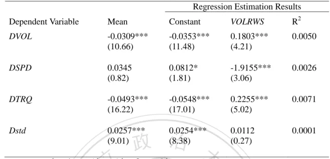
(20) In Table 12, the ARs of stocks on the expiration dates are not as significantly negative as the results in Table 11. A possible explanation is that investors would certainly exercise their call warrants in the expiration dates, so the issuers need no more stocks to hedge their short positions of warrants. They would sell their present holding positions in the stock market. Table 12 The Abnormal Returns of Stocks During the Expiration Dates of All Non-Deep In-the-money Warrants t-3. t-2. Mean. 0.0810***. 0.1086***. Std.. 2.1529. 2.2242. t-value. 3.87. t. t+1. t+2. t+3. 0.0010 0.0440** 政治大 2.1400 2.1527 2.0526. -0.0169. -0.0363*. 2.1083. 2.0585. 0.48. 0.82. 1.81. -0.0100. ‧ 國. 0.05 10553. 2.20. 學. N. 立 5.01. t-1. ‧. Day t is the expiration dates of warrants. The abnormal returns (ARs) of stocks are the daily returns of underlying stocks minus the daily market returns. The sample comprises 10553 non-deep in-the-money warrants over the period 2006-2010. ***, **, and * indicate significant level 1%, 5%, and 10%, respectively.. y. Nat. al. er. io. stock market in different levels of investor sentiment.. sit. In the following sections, we discuss further how the warrant market affects the. n. v i n C. Liquidity Change and C Cumulative h e n g cAbnormal h i U Returns The results in Table 13 show that the mean DVOL is －0.0309 with t＝10.66, highly significant. The coefficient of VOLRWS is significantly positive. It means if the average daily trading volume of warrants relative to the average daily trading volume of the stock before the (days －30 to －1) warrant expired raise, the trading volume of stocks relative to the market volume would also raise. Even though the mean of DVOL is negative, the increase in average stock volume is significantly induced by the decrease of numbers of living warrants. The mean DSPD is positive but insignificant. We could see the coefficient of. 15.

(21) VOLRWS is significantly negative. It is consistent with the results of DVOL which means that the greater the trading volume of warrants is, the greater the trading volume of the underlying stock is. And it also improved the liquidity of the stock market since the bid-ask spread decreased. Then we could see the mean DTRQ is －0.0493 with t＝16.22, highly significant. However, the coefficient of VOLRWS is significantly positive which represents that the liquidity of the stock market is indeed improved. Finally, the average Dstd is significantly positive. It means that the market depth of. 政治大. the stock market is poorer after the warrants expired, but the coefficient of VOLRWS is. 立. insignificant.. ‧. ‧ 國. 學. n. er. io. sit. y. Nat. al. Ch. engchi. 16. i n U. v.

(22) Table 13 Changes in The stock liquidity following the warrant Exercise Regression Estimation Results Dependent Variable. Mean. Constant. VOLRWS. R2. DVOL. -0.0309*** (10.66). -0.0353*** (11.48). 0.1803*** (4.21). 0.0050. DSPD. 0.0345 (0.82). 0.0812* (1.81). -1.9155*** (3.06). 0.0026. DTRQ. -0.0493*** (16.22). -0.0548*** (17.01). 0.2255*** (5.02). 0.0071. Dstd. 0.0257*** (9.01). 0.0254*** (8.38). 0.0112 (0.27). 0.0001. 立. 政治大. ‧ 國. 學. 𝐷𝑉𝑂𝐿𝑗 = 𝑙𝑜𝑔�𝑉𝑂𝐿𝑗𝐴 ∕ 𝑉𝑂𝐿𝐴𝑚 � − 𝑙𝑜𝑔�𝑉𝑂𝐿𝑗𝐵 ∕ 𝑉𝑂𝐿𝐵𝑚 �. VOL is the average daily volume, and j and m indicate stock j and the market, respectively. A indicates the period of 30 trading days after the warrant expiration, days ＋1 to ＋30, and B indicates the period of 30 days before expiration, days －30 to －1. 𝐷𝑆𝑃𝐷𝑗 = 𝑆𝑃𝑅𝐸𝐴𝐷𝑗𝐴 − 𝑆𝑃𝑅𝐸𝐴𝐷𝑗𝐵 . Roll (1984) proposes that 𝑆𝑃𝑅𝐸𝐴𝐷𝑗 = 2 ∙ �−𝐶𝑂𝑉𝑗 , where COV is the 𝑇𝑅𝑄𝑗𝐴. first order autocovariance of daily stock returns (multiplied by 100). 𝐷𝑇𝑅𝑄𝑗 = 𝑙𝑜𝑔 � 𝑇𝑟𝑎𝑑𝑖𝑛𝑔 𝑉𝑜𝑙𝑢𝑚𝑒𝑗. 𝑆h𝑎𝑟𝑒𝑠 𝑂𝑢𝑡𝑠𝑡𝑎𝑛𝑑𝑖𝑛𝑔𝑗. . 𝐷𝑠𝑡𝑑𝑗 = 𝑙𝑜𝑔 �. 𝑠𝑡𝑑.. � − 𝑙𝑜𝑔 �. 𝑇𝑟𝑎𝑑𝑖𝑛𝑔 𝑉𝑜𝑙𝑢𝑚𝑒 𝐴. 𝑠𝑡𝑑.. ‧. 𝑇𝑅𝑄𝑗 =. 𝑇𝑅𝑄𝑗𝐵. �, where. � . VOLRWS is the. 𝑇𝑟𝑎𝑑𝑖𝑛𝑔 𝑉𝑜𝑙𝑢𝑚𝑒 𝐵. n. al. er. io. sit. y. Nat. ratio of the average daily trading volume of warrants to that of the stock in the period of 30 trading days (days －30 to －1) before the warrant expired. The sample comprises 3549 warrants exercise over the period 2006-2010. The estimated models are (7) 𝐷𝐿𝐼𝑄𝑈𝐼𝐷𝐼𝑇𝑌𝑗 = 𝛾0 + 𝛾1 𝑉𝑂𝐿𝑅𝑊𝑆𝑗 + 𝑢𝑗 , Where DLIQUIDITYj＝DVOLj, DSPDj, DTRQj, or Dstdj. t-statistics are in parentheses. The t-statistics if the regression coefficients are calculated using robust estimation of the standard errors, following White (1980). ***, **, and * indicate significant level 1%, 5%, and 10%, respectively.. Ch. engchi. i n U. v. Table 14 shows how all the factors we use above affect the CAR. Our main test is whether stock prices are affected by the warrants expired. Hypothesis H1 could be explained as following reasons. According to the results in Table 13, we have noticed that the trading volume would transfer from warrants to stocks. The liquidity of the stock market increased after the warrants expired. The ensuing improvement in liquidity should bring higher stock prices (Amihud and Mendelson (1986), Brennan and Subrahmanyam (1996), Amihud, Mendelson, and Lauterbach (1997)).. 17.

(23) However, according to the results in Table 11, the mean value of the CAR is significantly negative. So we further study the relation between the CAR and the liquidity of stocks by examining Hypothesis H3. In Table 14, the coefficients of DVOL are significantly positive in the model (1) and (3). It is consistent with Hypothesis H3 which suggests that the coefficient of DVOL should be positive. If investors anticipate that the consolidation of trading between the warrants and the stocks improves liquidity, the increase in stock price should be an increasing function of the increase in its trading volume.. 立. 政治大. ‧. ‧ 國. 學. n. er. io. sit. y. Nat. al. Ch. engchi. 18. i n U. v.

(24) Table 14 Determinants of the Cumulative Abnormal Return (CAR) on the Expiration of All Deep-in-the-Money Warrants (3). (4). (5). (6). (7). (8). (9). -0.0718. -0.1057**. -0.0713. -0.0680. -0.0538. -0.0583. -0.0695. -0.0615. -0.0687. (1.45). (2.16). (1.44). (1.37). (1.06). (1.15). (1.41). (1.24). (1.38). 1.0564***. 1.1233***. (3.73). (3.94) 0.0363*. 0.0443**. (1.87). (2.27). R. 1.0273***. 0.0039. 0.0010. 0.0053. (1.42). 0.6222. (3.81). io. 2. (2.27). Nat. DVOLRAT. (0.93). 立 0.0443**. (1.21). ‧. Dstd. 0.4749. 學. DTRQ. 0.5005. 1.1327*** (3.98). al. -1.3591***. -1.1001***. (4.73). (3.23) 1.0661***. y. DSPD. 政治大. sit. DVOL. (2). 0.0054. 0.0041. 0.0043. er. Constant. (1). ‧ 國. Model. (3.77) 0.0063. 0.0068. 0.0040. 𝑙𝑜𝑔�𝑉𝑂𝐿𝑗𝐴. v. n. The dependent variable is CAR, the cumulative abnormal return over days (－1, 0), where day 0 is the warrant expiration dates. 𝐷𝑉𝑂𝐿𝑗 = ∕ 𝑉𝑂𝐿𝐴𝑚 � − 𝑙𝑜𝑔�𝑉𝑂𝐿𝑗𝐵 ∕ 𝑉𝑂𝐿𝐵𝑚 �. VOL is the average daily volume, and j and m indicate stock j and the market, respectively. A indicates the period of 30 trading days after the warrant expiration, days ＋1 to ＋30, and B indicates the period of 30 days before expiration, days －30 to －1. 𝐷𝑆𝑃𝐷𝑗 = 𝑆𝑃𝑅𝐸𝐴𝐷𝑗𝐴 − 𝑆𝑃𝑅𝐸𝐴𝐷𝑗𝐵 . Roll (1984) proposes that. Ch. engchi. i n U. 𝑇𝑅𝑄𝑗𝐴. 𝑆𝑃𝑅𝐸𝐴𝐷𝑗 = 2 ∙ �−𝐶𝑂𝑉𝑗 , where COV is the first order autocovariance of daily stock returns (multiplied by 100). 𝐷𝑇𝑅𝑄𝑗 = 𝑙𝑜𝑔 �. 𝐷𝑠𝑡𝑑𝑗 = 𝑙𝑜𝑔 �. 𝑠𝑡𝑑.. � − 𝑙𝑜𝑔 �. 𝑇𝑟𝑎𝑑𝑖𝑛𝑔 𝑉𝑜𝑙𝑢𝑚𝑒 𝐴. 𝑠𝑡𝑑.. 𝑇𝑅𝑄𝑗𝐵. �, where 𝑇𝑅𝑄𝑗 =. 𝑇𝑟𝑎𝑑𝑖𝑛𝑔 𝑉𝑜𝑙𝑢𝑚𝑒𝑗. 𝑆h𝑎𝑟𝑒𝑠 𝑂𝑢𝑡𝑠𝑡𝑎𝑛𝑑𝑖𝑛𝑔𝑗. � . 𝐷𝑉𝑂𝐿𝑅𝐴𝑇𝑗 = 𝐷𝑉𝑂𝐿𝑗 − 𝑙𝑜𝑔�1 + 𝑅𝐴𝑇𝑊𝑆𝑗 � , the excess of the post-exercise increase in the stock trading volume. 𝑇𝑟𝑎𝑑𝑖𝑛𝑔 𝑉𝑜𝑙𝑢𝑚𝑒 𝐵. over the post-exercise increase in number of shares. The sample comprises 3549 warrants exercise over the period 2006-2010. t-statistics are in parentheses. The t-statistics if the regression coefficients are calculated using robust estimation of the standard errors, following White (1980). ***, **, and * indicate significant level 1%, 5%, and 10%, respectively.. 19. ..

(25) The second measure is bid-ask spread, DSPD. In model (2), (3), and (4), the coefficients of DSPD are all significantly positive. It is consistent with Hypothesis H2 but contrary to Hypothesis H3. Then we could see the coefficients of the third and forth measures in model (5), (6), (7), and (8). Hypothesis H3 suggests that the coefficients of DTRQ and Dstd should be positive and negative, respectively. The higher the turnover rate is, the higher CAR is. It represents that the consolidation of trading improves liquidity, and further benefits CAR. Similarly, the deeper the market depth is, the higher CAR is.. 治政大 increases after the warrant RATWS. Since the number of shares of stocks naturally 立. The fifth measure is DVOLRAT, which is the difference between DVOL and. exercise, it may be expected that the trading volume of stocks would increase as well.. ‧ 國. 學. However, most of warrants use cash to implement the contracts instead of using stocks.. ‧. Besides, part of the trading volume in the stocks may be due to arbitrage or hedge. sit. y. Nat. transactions between stocks and warrants. We obtain that the mean of DVOLRAT is －. io. n. al. er. 0.0335 with t＝11.57, significantly different from zero, and the median is －0.0363,. i n U. v. implying that the trading volume of most stocks increases by less than the increase in the. Ch. engchi. number of shares of stock after the warrants expired. The result inflects that the part of the trading volume before warrants exercise is due to arbitrage or hedge trading. The coefficients of DVOLRAT are significantly positive in model (4) and (9). The results are consistent with Hypothesis H3.. 20.

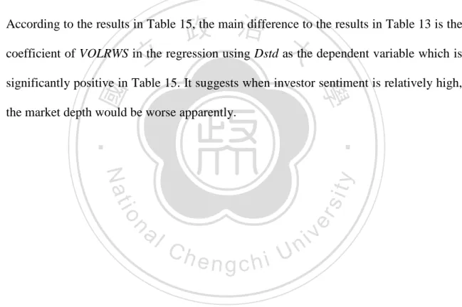
(26) D. Investor Sentiment In this section, we want to see if there is any results change in different levels of investor sentiment. We use VIX as a proxy to measure investor sentiment. As we mentioned in the previous section, we use the mean value of VIX in the whole sample period as a criterion to define the period of high VIX and low VIX. Table 15 shows changes in the stock liquidity following the warrant exercise in the high VIX period which we calculate the mean value of VIX during the period of 30 trading days before and after the expiration dates following the window of (－30, ＋30).. 政治大 coefficient of VOLRWS in the regression using Dstd as the dependent variable which is 立. According to the results in Table 15, the main difference to the results in Table 13 is the. ‧ 國. 學. significantly positive in Table 15. It suggests when investor sentiment is relatively high, the market depth would be worse apparently.. ‧. n. er. io. sit. y. Nat. al. Ch. engchi. 21. i n U. v.

(27) Table 15 Changes in The stock liquidity following the warrant Exercise in the Period of High VIX Regression Estimation Results Dependent Variable. Mean. Constant. VOLRWS. R2. DVOL. -0.0138*** (3.32). -0.0152*** (3.50). 0.0870 (1.12). 0.0011. DSPD. 0.2497*** (2.91). 0.2961*** (3.31). -2.8384* (1.78). 0.0028. DTRQ. -0.0669*** (15.07). -0.0675*** (14.53). 0.0348 (0.42). 0.0002. Dstd. 0.0125** (3.05). 0.2951*** (3.89). 0.0132. 立. 政治 0.0077* 大 (1.80). ‧. ‧ 國. 學. 𝐷𝑉𝑂𝐿𝑗 = 𝑙𝑜𝑔�𝑉𝑂𝐿𝑗𝐴 ∕ 𝑉𝑂𝐿𝐴𝑚 � − 𝑙𝑜𝑔�𝑉𝑂𝐿𝑗𝐵 ∕ 𝑉𝑂𝐿𝐵𝑚 �. VOL is the average daily volume, and j and m indicate stock j and the market, respectively. A indicates the period of 30 trading days after the warrant expiration, days ＋1 to ＋30, and B indicates the period of 30 days before expiration, days －30 to －1. 𝐷𝑆𝑃𝐷𝑗 = 𝑆𝑃𝑅𝐸𝐴𝐷𝑗𝐴 − 𝑆𝑃𝑅𝐸𝐴𝐷𝑗𝐵 . Roll (1984) proposes that 𝑆𝑃𝑅𝐸𝐴𝐷𝑗 = 2 ∙ �−𝐶𝑂𝑉𝑗 , where COV is the 𝑇𝑅𝑄𝑗𝐴. first order autocovariance of daily stock returns (multiplied by 100). 𝐷𝑇𝑅𝑄𝑗 = 𝑙𝑜𝑔 � . 𝐷𝑠𝑡𝑑𝑗 = 𝑙𝑜𝑔 �. 𝑠𝑡𝑑.. � − 𝑙𝑜𝑔 �. 𝑇𝑟𝑎𝑑𝑖𝑛𝑔 𝑉𝑜𝑙𝑢𝑚𝑒 𝐴. 𝑠𝑡𝑑.. y. 𝑆h𝑎𝑟𝑒𝑠 𝑂𝑢𝑡𝑠𝑡𝑎𝑛𝑑𝑖𝑛𝑔𝑗. �, where. � . VOLRWS is the. 𝑇𝑟𝑎𝑑𝑖𝑛𝑔 𝑉𝑜𝑙𝑢𝑚𝑒 𝐵. sit. 𝑇𝑟𝑎𝑑𝑖𝑛𝑔 𝑉𝑜𝑙𝑢𝑚𝑒𝑗. Nat. 𝑇𝑅𝑄𝑗 =. 𝑇𝑅𝑄𝑗𝐵. n. al. er. io. ratio of the average daily trading volume of warrants to that of the stock in the period of 30 trading days (days －30 to －1) before the warrant expired. The sample comprises 1138 warrants in the period of high VIX (we calculate the mean value of VIX during the period of 30 trading days before and after the expiration dates following the window of (－30, ＋30)) exercise over 2006-2010. The estimated models are (7) 𝐷𝐿𝐼𝑄𝑈𝐼𝐷𝐼𝑇𝑌𝑗 = 𝛾0 + 𝛾1 𝑉𝑂𝐿𝑅𝑊𝑆𝑗 + 𝑢𝑗 , Where DLIQUIDITYj＝DVOLj, DSPDj, DTRQj, or Dstdj. t-statistics are in parentheses. The t-statistics if the regression coefficients are calculated using robust estimation of the standard errors, following White (1980). ***, **, and * indicate significant level 1%, 5%, and 10%, respectively.. Ch. engchi. i n U. v. Besides, the coefficients of DVOL and DTRQ are insignificant different from zero. It means that the effect of improvements in the stock liquidity is getting insignificant in the period of high VIX. Further, we could see the relation between CAR and variables during the period of high VIX. We obtain that the mean of CAR in Table 16 is －0.1405 with t＝1.46, insignificantly different from zero. The coefficients of the first measure of liquidity,. 22.

(28) DVOL, are still significantly positive in model (1) and (3) as well as the results in Table 14. However, the coefficients of DSPD are insignificant in model (2), (3), and (4). These results are different to those in Table 14. It means that Hypothesis H2 is weaker in the period of high VIX. Then we could check the coefficients of DTRQ, Dstd, and DVOLRAT, they are all consistent with the results in Table 14. Going a step further, we could see that the moduli are bigger than the results in the whole sample period. It suggests that investors are more sensitive in the period of high VIX.. 立. 政治大. ‧. ‧ 國. 學. n. er. io. sit. y. Nat. al. Ch. engchi. 23. i n U. v.

(29) Table 16 Determinants of the Cumulative Abnormal Return (CAR) on the Expiration of All Deep-in-the-Money Warrants in the Period of High VIX. DVOL. (2). (3). (4). (5). (6). (7). (8). (9). -0.1207. -0.1497. -0.1304. -0.1267. -0.0248. -0.0099. -0.1083. -0.1087. -0.1171. (1.25). (1.55). (1.35). (1.30). (0.24). (0.09). (1.13). (1.13). (1.21). 1.4314**. 1.5008**. (2.09). (2.18) 0.0370. 0.0428. (1.11). (1.28). 0.0038. 0.0011. (0.07). 2.0301*. (2.70). (1.73). 1.4875** (2.17). 0.0053. io. R. 2. 1.7294***. Nat. DVOLRAT. (0.31). ‧. Dstd. -0.0608. 學. DTRQ. -0.3829. 立 (1.28). ‧ 國. DSPD. 政治大 0.0427. -2.5776***. -2.6137***. (3.71). (3.06) 1.4184**. y. Constant. (1). 0.0052. sit. Model. 0.0064. 0.0064. (2.07) 0.0120. 0.0120. 0.0038. 𝑙𝑜𝑔�𝑉𝑂𝐿𝑗𝐴. n. al. er. The dependent variable is CAR, the cumulative abnormal return over days (－1, 0), where day 0 is the warrant expiration dates. 𝐷𝑉𝑂𝐿𝑗 = ∕ 𝑉𝑂𝐿𝐴𝑚 � − 𝑙𝑜𝑔�𝑉𝑂𝐿𝑗𝐵 ∕ 𝑉𝑂𝐿𝐵𝑚 �. VOL is the average daily volume, and j and m indicate stock j and the market, respectively. A indicates the period of 30 trading days after the warrant expiration, days ＋1 to ＋30, and B indicates the period of 30 days before expiration, days －30 to －1. 𝐷𝑆𝑃𝐷𝑗 = 𝑆𝑃𝑅𝐸𝐴𝐷𝑗𝐴 − 𝑆𝑃𝑅𝐸𝐴𝐷𝑗𝐵 . Roll (1984) proposes that. Ch. engchi. i n U. v. 𝑇𝑅𝑄𝑗𝐴. 𝑆𝑃𝑅𝐸𝐴𝐷𝑗 = 2 ∙ �−𝐶𝑂𝑉𝑗 , where COV is the first order autocovariance of daily stock returns (multiplied by 100). 𝐷𝑇𝑅𝑄𝑗 = 𝑙𝑜𝑔 �. 𝐷𝑠𝑡𝑑𝑗 = 𝑙𝑜𝑔 �. 𝑠𝑡𝑑.. � − 𝑙𝑜𝑔 �. 𝑇𝑟𝑎𝑑𝑖𝑛𝑔 𝑉𝑜𝑙𝑢𝑚𝑒 𝐴. 𝑠𝑡𝑑.. 𝑇𝑅𝑄𝑗𝐵. �, where 𝑇𝑅𝑄𝑗 =. 𝑇𝑟𝑎𝑑𝑖𝑛𝑔 𝑉𝑜𝑙𝑢𝑚𝑒𝑗. 𝑆h𝑎𝑟𝑒𝑠 𝑂𝑢𝑡𝑠𝑡𝑎𝑛𝑑𝑖𝑛𝑔𝑗. � . 𝐷𝑉𝑂𝐿𝑅𝐴𝑇𝑗 = 𝐷𝑉𝑂𝐿𝑗 − 𝑙𝑜𝑔�1 + 𝑅𝐴𝑇𝑊𝑆𝑗 � , the excess of the post-exercise increase in the stock trading volume. 𝑇𝑟𝑎𝑑𝑖𝑛𝑔 𝑉𝑜𝑙𝑢𝑚𝑒 𝐵. .. over the post-exercise increase in number of shares. The sample comprises 1138 warrants in the period of high VIX (we calculate the mean value of VIX during the period of 30 trading days before and after the expiration dates following the window of (－30, ＋30)) exercise over 2006-2010. t-statistics are in parentheses. The t-statistics if the regression coefficients are calculated using robust estimation of the standard errors, following White (1980). ***, **, and * indicate significant level 1%, 5%, and 10%, respectively.. 24.

(30) In Table 17, we could find out that the mean value of DSPD is insignificantly negative during the period of low VIX which we calculate the mean value of VIX during the period of 30 trading days before and after the expiration dates following the window of (－30, ＋30). Comparing with the results in the period of high VIX, we could see the coefficients of VOLRWS get much more significant in Table 17. It reveals that the stock liquidity is improved after the warrants expired. The results are more robust in the period of low VIX. Table 17. 政 VIX治大. Changes in The stock liquidity following the warrant Exercise in the Period of Low. 立. Regression Estimation Results Constant VOLRWS R2 -0.0452*** 0.2235*** 0.0077 (11.22) (4.33). DSPD. -0.0670 (1.42). -0.0257 (0.51). -0.0410*** (10.40). -0.0483*** (11.47). 0.0021. sit. y. -1.4696** (2.27). a0.0319*** 0.0340*** i v l C n (8.57) h (8.53) U engchi. n. 0.2576*** (4.78). 0.0094. -0.0751 (1.47). 0.0009. er. io. Dstd. ‧. Nat. DTRQ. ‧ 國. Mean -0.0389*** (10.31). 學. Dependent Variable DVOL. 𝐷𝑉𝑂𝐿𝑗 = 𝑙𝑜𝑔�𝑉𝑂𝐿𝑗𝐴 ∕ 𝑉𝑂𝐿𝐴𝑚 � − 𝑙𝑜𝑔�𝑉𝑂𝐿𝑗𝐵 ∕ 𝑉𝑂𝐿𝐵𝑚 �. VOL is the average daily volume, and j and m indicate stock j and the market, respectively. A indicates the period of 30 trading days after the warrant expiration, days ＋1 to ＋30, and B indicates the period of 30 days before expiration, days －30 to －1. 𝐷𝑆𝑃𝐷𝑗 = 𝑆𝑃𝑅𝐸𝐴𝐷𝑗𝐴 − 𝑆𝑃𝑅𝐸𝐴𝐷𝑗𝐵 . Roll (1984) proposes that 𝑆𝑃𝑅𝐸𝐴𝐷𝑗 = 2 ∙ �−𝐶𝑂𝑉𝑗 , where COV is the 𝑇𝑅𝑄𝑗𝐴. first order autocovariance of daily stock returns (multiplied by 100). 𝐷𝑇𝑅𝑄𝑗 = 𝑙𝑜𝑔 �. 𝑇𝑅𝑄𝑗 =. 𝑇𝑟𝑎𝑑𝑖𝑛𝑔 𝑉𝑜𝑙𝑢𝑚𝑒𝑗. 𝑆h𝑎𝑟𝑒𝑠 𝑂𝑢𝑡𝑠𝑡𝑎𝑛𝑑𝑖𝑛𝑔𝑗. . 𝐷𝑠𝑡𝑑𝑗 = 𝑙𝑜𝑔 �. 𝑠𝑡𝑑.. � − 𝑙𝑜𝑔 �. 𝑇𝑟𝑎𝑑𝑖𝑛𝑔 𝑉𝑜𝑙𝑢𝑚𝑒 𝐴. 𝑠𝑡𝑑.. 𝑇𝑅𝑄𝑗𝐵. �, where. � . VOLRWS is the. 𝑇𝑟𝑎𝑑𝑖𝑛𝑔 𝑉𝑜𝑙𝑢𝑚𝑒 𝐵. ratio of the average daily trading volume of warrants to that of the stock in the period of 30 trading days (days －30 to －1) before the warrant expired. The sample comprises 2411 warrants in the period of low VIX (we calculate the mean value of VIX during the period of 30 trading days before and after the expiration dates following the window of (－30, ＋30)) exercise over 2006-2010. The estimated models are (7) 𝐷𝐿𝐼𝑄𝑈𝐼𝐷𝐼𝑇𝑌𝑗 = 𝛾0 + 𝛾1 𝑉𝑂𝐿𝑅𝑊𝑆𝑗 + 𝑢𝑗 , Where DLIQUIDITYj＝DVOLj, DSPDj, DTRQj, or Dstdj. t-statistics are in parentheses. The t-statistics if the regression coefficients are calculated using robust estimation of the standard errors, following White (1980). ***, **, and * indicate significant level 1%, 5%, and 10%, respectively.. 25.

(31) In Table 18, we obtain that the mean of CAR is － 0.0874 with t ＝ 1.56, insignificantly different from zero as well as the results in the period of high VIX. Nevertheless, we could still see the coefficients of DVOL, DTRQ, Dstd, and DVOLRAT are significant in most of models, although the mean of CAR is insignificantly different form zero. Further, we could find out that the moduli of the coefficients are lower than those in the whole sample and high VIX period apparently. The coefficients of DSPD get more insignificant in the period of low VIX comparing with the whole sample period. So we could infer that Hypothesis H2 is only established. 政治大 VIX, the strength of Hypothesis H2 gets worse. In contrast, Hypothesis H3 is established 立. in the whole sample period. If we separate the sample into the periods of high and low. ‧ 國. 學. in any period of the sample, especially more robust in the period of high VIX. Next section we will go further to separate the sample into different levels of investor. ‧. sentiment around warrants expiration.. n. er. io. sit. y. Nat. al. Ch. engchi. 26. i n U. v.

(32) Table 18 Determinants of the Cumulative Abnormal Return (CAR) on the Expiration of All Deep-in-the-Money Warrants in the Period of Low VIX. DVOL. (2). (3). (4). (5). (6). (7). (8). (9). -0.0496. -0.0850. -0.0435. -0.0400. -0.0536. -0.0491. -0.0540. -0.0409. -0.0463. (0.87). (1.52). (0.76). (0.70). (0.94). (0.86). (0.95). (0.72). (0.81). 0.9734***. 1.0476***. (3.23). (3.45) 0.0370. 0.0475*. (1.53). (1.95). 0.0043. 0.0010. (0.13). 1.0632*** (3.50). 0.0059. (1.69). 0.0762. (2.86). io. R. (1.51). (1.90) 0.8235***. Nat. DVOLRAT. 0.5967*. ‧. Dstd. 0.9044. 學. DTRQ. 2. 立. ‧ 國. DSPD. 政治大 0.0476*. -1.0467***. -0.7304**. (3.43). (2.04) 0.9891***. y. Constant. (1). 0.0060. sit. Model. 0.0034. 0.0043. (3.28) 0.0048. 0.0060. 0.0045. 𝑙𝑜𝑔�𝑉𝑂𝐿𝑗𝐴. n. al. er. The dependent variable is CAR, the cumulative abnormal return over days (－1, 0), where day 0 is the warrant expiration dates. 𝐷𝑉𝑂𝐿𝑗 = ∕ 𝑉𝑂𝐿𝐴𝑚 � − 𝑙𝑜𝑔�𝑉𝑂𝐿𝑗𝐵 ∕ 𝑉𝑂𝐿𝐵𝑚 �. VOL is the average daily volume, and j and m indicate stock j and the market, respectively. A indicates the period of 30 trading days after the warrant expiration, days ＋1 to ＋30, and B indicates the period of 30 days before expiration, days －30 to －1. 𝐷𝑆𝑃𝐷𝑗 = 𝑆𝑃𝑅𝐸𝐴𝐷𝑗𝐴 − 𝑆𝑃𝑅𝐸𝐴𝐷𝑗𝐵 . Roll (1984) proposes that. Ch. engchi. i n U. v. 𝑇𝑅𝑄𝑗𝐴. 𝑆𝑃𝑅𝐸𝐴𝐷𝑗 = 2 ∙ �−𝐶𝑂𝑉𝑗 , where COV is the first order autocovariance of daily stock returns (multiplied by 100). 𝐷𝑇𝑅𝑄𝑗 = 𝑙𝑜𝑔 �. 𝐷𝑠𝑡𝑑𝑗 = 𝑙𝑜𝑔 �. 𝑠𝑡𝑑.. � − 𝑙𝑜𝑔 �. 𝑇𝑟𝑎𝑑𝑖𝑛𝑔 𝑉𝑜𝑙𝑢𝑚𝑒 𝐴. 𝑠𝑡𝑑.. 𝑇𝑅𝑄𝑗𝐵. �, where 𝑇𝑅𝑄𝑗 =. 𝑇𝑟𝑎𝑑𝑖𝑛𝑔 𝑉𝑜𝑙𝑢𝑚𝑒𝑗. 𝑆h𝑎𝑟𝑒𝑠 𝑂𝑢𝑡𝑠𝑡𝑎𝑛𝑑𝑖𝑛𝑔𝑗. � . 𝐷𝑉𝑂𝐿𝑅𝐴𝑇𝑗 = 𝐷𝑉𝑂𝐿𝑗 − 𝑙𝑜𝑔�1 + 𝑅𝐴𝑇𝑊𝑆𝑗 � , the excess of the post-exercise increase in the stock trading volume. 𝑇𝑟𝑎𝑑𝑖𝑛𝑔 𝑉𝑜𝑙𝑢𝑚𝑒 𝐵. over the post-exercise increase in number of shares. The sample comprises 2411 warrants in the period of low VIX (we calculate the mean value of VIX during the period of 30 trading days before and after the expiration dates following the window of (－30, ＋30)) exercise over 2006-2010. t-statistics are in parentheses. The t-statistics if the regression coefficients are calculated using robust estimation of the standard errors, following White (1980). ***, **, and * indicate significant level 1%, 5%, and 10%, respectively.. 27. ..

(33) E. The Change in Investor Sentiment In this section, we calculate the mean values of VIX before and after warrants expiration respectively. Using the same criteria we use in the section B, if the mean value of VIX is higher than 26.85, we define it as the period of high VIX. Otherwise, we define it as the period of low VIX. First, comparing with the whole sample period, we could observe how the liquidity of stocks and CAR would be affected if VIX around warrants expiration are both relatively lower. In Table 19, the significance of the mean values of all variables is. 政治大. consistent with the results in Table 13. The mean of DSPD is still insignificant. And the. 立. coefficients of VOLRWS in the regression using Dstd as the dependent variable changed. ‧ 國. 學. into negative significantly. It suggests when investor sentiments are both low around the expiration dates, Hypothesis H1 is much more robust. On the other hand, Hypothesis H2. ‧. gets weaker in this period.. n. er. io. sit. y. Nat. al. Ch. engchi. 28. i n U. v.

(34) Table 19 Changes in The stock liquidity following the warrant Exercise from the Period of Low VIX to Low VIX Regression Estimation Results Dependent Variable. Mean. Constant. VOLRWS. R2. DVOL. -0.0404*** (9.95). -0.0461*** (10.62). 0.1967*** (3.64). 0.0077. DSPD. -0.0157 (0.31). 0.0140 (0.26). -1.0277 (1.54). 0.0021. DTRQ. -0.0402*** (9.46). -0.0468*** (10.29). 0.2252*** (3.97). 0.0094. Dstd. 0.0287*** (7.13). -0.0917* (1.71). 0.0009. 立. 治政 0.0313*** (7.27) 大. ‧ 國. 學. 𝐷𝑉𝑂𝐿𝑗 = 𝑙𝑜𝑔�𝑉𝑂𝐿𝑗𝐴 ∕ 𝑉𝑂𝐿𝐴𝑚 � − 𝑙𝑜𝑔�𝑉𝑂𝐿𝑗𝐵 ∕ 𝑉𝑂𝐿𝐵𝑚 �. VOL is the average daily volume, and j and m indicate stock j and the market, respectively. A indicates the period of 30 trading days after the warrant expiration, days ＋1 to ＋30, and B indicates the period of 30 days before expiration, days －30 to －1. 𝐷𝑆𝑃𝐷𝑗 = 𝑆𝑃𝑅𝐸𝐴𝐷𝑗𝐴 − 𝑆𝑃𝑅𝐸𝐴𝐷𝑗𝐵 . Roll (1984) proposes that 𝑆𝑃𝑅𝐸𝐴𝐷𝑗 = 2 ∙ �−𝐶𝑂𝑉𝑗 , where COV is the 𝑇𝑅𝑄𝑗𝐴. 𝑇𝑅𝑄𝑗 =. 𝑇𝑟𝑎𝑑𝑖𝑛𝑔 𝑉𝑜𝑙𝑢𝑚𝑒𝑗. 𝑆h𝑎𝑟𝑒𝑠 𝑂𝑢𝑡𝑠𝑡𝑎𝑛𝑑𝑖𝑛𝑔𝑗. . 𝐷𝑠𝑡𝑑𝑗 = 𝑙𝑜𝑔 �. 𝑠𝑡𝑑.. � − 𝑙𝑜𝑔 �. 𝑇𝑟𝑎𝑑𝑖𝑛𝑔 𝑉𝑜𝑙𝑢𝑚𝑒 𝐴. ‧. first order autocovariance of daily stock returns (multiplied by 100). 𝐷𝑇𝑅𝑄𝑗 = 𝑙𝑜𝑔 � 𝑠𝑡𝑑.. 𝑇𝑅𝑄𝑗𝐵. �, where. � . VOLRWS is the. 𝑇𝑟𝑎𝑑𝑖𝑛𝑔 𝑉𝑜𝑙𝑢𝑚𝑒 𝐵. n. al. y. er. io. sit. Nat. ratio of the average daily trading volume of warrants to that of the stock in the period of 30 trading days (days －30 to －1) before the warrant expired. The sample comprises 2138 warrants from the period of low VIX to low VIX (we calculate the mean value of VIX during the period of 30 trading days before and after the expiration dates following the window of (－30, ＋30)) exercise over 2006-2010. The estimated models are (7) 𝐷𝐿𝐼𝑄𝑈𝐼𝐷𝐼𝑇𝑌𝑗 = 𝛾0 + 𝛾1 𝑉𝑂𝐿𝑅𝑊𝑆𝑗 + 𝑢𝑗 , Where DLIQUIDITYj＝DVOLj, DSPDj, DTRQj, or Dstdj. t-statistics are in parentheses. The t-statistics if the regression coefficients are calculated using robust estimation of the standard errors, following White (1980). ***, **, and * indicate significant level 1%, 5%, and 10%, respectively.. Ch. engchi. i n U. v. Then we could see how the variables affect CAR in the low VIX around the expiration dates in Table 20. We obtain the mean of CAR is －0.0840 with t＝1.44, insignificantly different from zero. Comparing the results with those in Table 14, although the coefficients of DSPD and the mean of CAR are insignificant in Table 20, it is much supportable to Hypothesis H3.. 29.

(35) Table 20 Determinants of the Cumulative Abnormal Return (CAR) on the Expiration of All Deep-in-the-Money Warrants from the Period of Low VIX to Low VIX (3). (4). (5). (6). (7). (8). (9). -0.0348. -0.0836. -0.0323. -0.0284. -0.04370. -0.0347. -0.0522. -0.0296. -0.0310. (0.59). (1.43). (0.54). (0.48). (0.74). (0.58). (0.89). (0.50). (0.52). 1.2181***. 1.2661***. (3.93). (4.06) 0.0359. 立 0.0360. (0.97). (1.42). (1.42). DTRQ. 2. 0.0072. 0.0004. (2.45). 0.0164. (3.39). (0.03). 1.2822*** (4.12). 0.0081. io. R. 1.0020***. Nat. DVOLRAT. (1.99). ‧. Dstd. 0.8858**. 學. 0.0247. 1.2033**. -1.1115***. -0.6488**. (3.55). (1.78) 1.2343***. y. DSPD. 政治大. 0.0083. 0.0053. sit. DVOL. (2). 0.0072. er. Constant. (1). ‧ 國. Model. (3.99) 0.0059. 0.0087. 0.0074. The dependent variable is CAR, the cumulative abnormal return over days (－1, 0), where day 0 is the warrant expiration dates. 𝐷𝑉𝑂𝐿𝑗 = 𝑙𝑜𝑔�𝑉𝑂𝐿𝑗𝐴 ∕ 𝑉𝑂𝐿𝐴𝑚 � − 𝑙𝑜𝑔�𝑉𝑂𝐿𝑗𝐵 ∕ 𝑉𝑂𝐿𝐵𝑚 �. VOL is the average daily volume, and j and m indicate stock j and the market, respectively. A indicates the period of 30 trading days after the warrant expiration, days ＋1 to ＋30, and B indicates the period of 30 days before expiration, days －30 to －1. 𝐷𝑆𝑃𝐷𝑗 = 𝑆𝑃𝑅𝐸𝐴𝐷𝑗𝐴 − 𝑆𝑃𝑅𝐸𝐴𝐷𝑗𝐵 . Roll (1984) proposes that. n. al. Ch. engchi. i n U. v. 𝑇𝑅𝑄𝑗𝐴. 𝑆𝑃𝑅𝐸𝐴𝐷𝑗 = 2 ∙ �−𝐶𝑂𝑉𝑗 , where COV is the first order autocovariance of daily stock returns (multiplied by 100). 𝐷𝑇𝑅𝑄𝑗 = 𝑙𝑜𝑔 �. 𝐷𝑠𝑡𝑑𝑗 = 𝑙𝑜𝑔 �. 𝑠𝑡𝑑.. � − 𝑙𝑜𝑔 �. 𝑇𝑟𝑎𝑑𝑖𝑛𝑔 𝑉𝑜𝑙𝑢𝑚𝑒 𝐴. 𝑠𝑡𝑑.. 𝑇𝑅𝑄𝑗𝐵. �, where 𝑇𝑅𝑄𝑗 =. 𝑇𝑟𝑎𝑑𝑖𝑛𝑔 𝑉𝑜𝑙𝑢𝑚𝑒𝑗. 𝑆h𝑎𝑟𝑒𝑠 𝑂𝑢𝑡𝑠𝑡𝑎𝑛𝑑𝑖𝑛𝑔𝑗. � . 𝐷𝑉𝑂𝐿𝑅𝐴𝑇𝑗 = 𝐷𝑉𝑂𝐿𝑗 − 𝑙𝑜𝑔�1 + 𝑅𝐴𝑇𝑊𝑆𝑗 � , the excess of the post-exercise increase in the stock trading volume. 𝑇𝑟𝑎𝑑𝑖𝑛𝑔 𝑉𝑜𝑙𝑢𝑚𝑒 𝐵. over the post-exercise increase in number of shares. The sample comprises 2138 warrants from the period of low VIX to low VIX (we calculate the mean value of VIX during the period of 30 trading days before and after the expiration dates following the window of (－30, ＋30)) exercise over 2006-2010. t-statistics are in parentheses. The t-statistics if the regression coefficients are calculated using robust estimation of the standard errors, following White (1980). ***, **, and * indicate significant level 1%, 5%, and 10%, respectively.. 30. ..

(36) In Table 21, we focus on the sample of period from low VIX to high VIX. The mean values of DVOL and DSPD have different signs comparing with the whole sample period which is presented in Table 13. The mean of DVOL is positive but insignificant and the mean of DSPD becomes negative significantly. We further check the coefficient of VOLRWS, we could see they are all insignificant in Table 21. The effect of improving the liquidity of the stock market following the warrants expired is weaker here. We could explain it from the point of hedge trading. If investor sentiment gets high after the warrants expiration, investors may be reluctant to. 政治大. invest more since they have lost a hedging tool.. 立. ‧. ‧ 國. 學. n. er. io. sit. y. Nat. al. Ch. engchi. 31. i n U. v.

(37) Table 21 Changes in The stock liquidity following the warrant Exercise from the Period of Low VIX to High VIX Regression Estimation Results Dependent Variable. Mean. Constant. VOLRWS. R2. DVOL. 0.0097 (0.52). 0.01266 (0.56). -0.0395 (0.23). 0.0006. DSPD. -1.0275*** (3.34). -0.7832** (2.09). -3.2315 (1.14). 0.0135. DTRQ. -0.0384* (1.82). -0.0187 (0.73). -0.2611 (1.34). 0.0186. Dstd. 0.1812*** (9.83). 0.1490 (0.87). 0.0080. 立. 𝐷𝑉𝑂𝐿𝑗 = ∕ − 𝑙𝑜𝑔�𝑉𝑂𝐿𝑗𝐵 ∕ 𝑉𝑂𝐿𝐵𝑚 �. VOL is the average daily volume, and j and m indicate stock j and the market, respectively. A indicates the period of 30 trading days after the warrant expiration, days ＋1 to ＋30, and B indicates the period of 30 days before expiration, days －30 to －1. 𝐷𝑆𝑃𝐷𝑗 = 𝑆𝑃𝑅𝐸𝐴𝐷𝑗𝐴 − 𝑆𝑃𝑅𝐸𝐴𝐷𝑗𝐵 . Roll (1984) proposes that 𝑆𝑃𝑅𝐸𝐴𝐷𝑗 = 2 ∙ �−𝐶𝑂𝑉𝑗 , where COV is the. ‧. ‧ 國. 𝑉𝑂𝐿𝐴𝑚 �. 學. 𝑙𝑜𝑔�𝑉𝑂𝐿𝑗𝐴. 0.1700*** 政治 (7.55) 大. 𝑇𝑅𝑄𝑗𝐴. first order autocovariance of daily stock returns (multiplied by 100). 𝐷𝑇𝑅𝑄𝑗 = 𝑙𝑜𝑔 � . 𝐷𝑠𝑡𝑑𝑗 = 𝑙𝑜𝑔 �. 𝑠𝑡𝑑.. � − 𝑙𝑜𝑔 �. 𝑇𝑟𝑎𝑑𝑖𝑛𝑔 𝑉𝑜𝑙𝑢𝑚𝑒 𝐴. 𝑠𝑡𝑑.. 𝑇𝑅𝑄𝑗𝐵. �, where. � . VOLRWS is the. 𝑇𝑟𝑎𝑑𝑖𝑛𝑔 𝑉𝑜𝑙𝑢𝑚𝑒 𝐵. y. 𝑆h𝑎𝑟𝑒𝑠 𝑂𝑢𝑡𝑠𝑡𝑎𝑛𝑑𝑖𝑛𝑔𝑗. Nat. 𝑇𝑅𝑄𝑗 =. 𝑇𝑟𝑎𝑑𝑖𝑛𝑔 𝑉𝑜𝑙𝑢𝑚𝑒𝑗. n. al. sit. er. io. ratio of the average daily trading volume of warrants to that of the stock in the period of 30 trading days (days －30 to －1) before the warrant expired. The sample comprises 97 warrants from the period of low VIX to high VIX (we calculate the mean value of VIX during the period of 30 trading days before and after the expiration dates following the window of (－30, ＋30)) exercise over 2006-2010. The estimated models are (7) 𝐷𝐿𝐼𝑄𝑈𝐼𝐷𝐼𝑇𝑌𝑗 = 𝛾0 + 𝛾1 𝑉𝑂𝐿𝑅𝑊𝑆𝑗 + 𝑢𝑗 , Where DLIQUIDITYj＝DVOLj, DSPDj, DTRQj, or Dstdj. t-statistics are in parentheses. The t-statistics if the regression coefficients are calculated using robust estimation of the standard errors, following White (1980). ***, **, and * indicate significant level 1%, 5%, and 10%, respectively.. Ch. engchi. i n U. v. Then we could see the results in Table 22 that the coefficients of variables are almost insignificant. Only in model (8), the coefficient of DVOL is negative significantly which means that the CAR is not an increasing function of liquidity. It is against Hypothesis H3, which indicated the liquidity of stock market benefits from consolidation of trading following the warrants expiration.. 32.

(38) Table 22 Determinants of the Cumulative Abnormal Return (CAR) on the Expiration of All Deep-in-the-Money Warrants from the Period of Low VIX to High VIX (3). (4). (5). (6). (7). (8). (9). -0.4367. -0.5132. -0.5345. -0.5475. -0.5138. -0.3239. -0.4183. 0.9406. -0.4485. (1.03). (1.14). (1.19). (1.22). (1.18). (0.72). (0.69). (1.15). (1.06). -3.2100. -3.6244. (1.37). (1.50). -0.0988. (0.31). (0.68). (0.68). 0.0195. 0.0010. (2.40). 2.4009. (0.58). (0.74). -3.5733 (1.48). 0.0243. io. R. -1.1994. Nat. DVOLRAT. (1.45). ‧. Dstd. -8.9091**. 學. -0.0992. DTRQ. 2. 立. -0.0443. -5.3307. -0.2727. -7.2969*. (0.12). (1.95) -3.1594. y. DSPD. 政治大. 0.0238. 0.0036. sit. DVOL. (2). 0.0252. er. Constant. (1). ‧ 國. Model. (1.36) 0.0001. 0.0578. 0.0190. The dependent variable is CAR, the cumulative abnormal return over days (－1, 0), where day 0 is the warrant expiration dates. 𝐷𝑉𝑂𝐿𝑗 = 𝑙𝑜𝑔�𝑉𝑂𝐿𝑗𝐴 ∕ 𝑉𝑂𝐿𝐴𝑚 � − 𝑙𝑜𝑔�𝑉𝑂𝐿𝑗𝐵 ∕ 𝑉𝑂𝐿𝐵𝑚 �. VOL is the average daily volume, and j and m indicate stock j and the market, respectively. A indicates the period of 30 trading days after the warrant expiration, days ＋1 to ＋30, and B indicates the period of 30 days before expiration, days －30 to －1. 𝐷𝑆𝑃𝐷𝑗 = 𝑆𝑃𝑅𝐸𝐴𝐷𝑗𝐴 − 𝑆𝑃𝑅𝐸𝐴𝐷𝑗𝐵 . Roll (1984) proposes that. n. al. Ch. engchi. i n U. v. 𝑇𝑅𝑄𝑗𝐴. 𝑆𝑃𝑅𝐸𝐴𝐷𝑗 = 2 ∙ �−𝐶𝑂𝑉𝑗 , where COV is the first order autocovariance of daily stock returns (multiplied by 100). 𝐷𝑇𝑅𝑄𝑗 = 𝑙𝑜𝑔 �. 𝐷𝑠𝑡𝑑𝑗 = 𝑙𝑜𝑔 �. 𝑠𝑡𝑑.. � − 𝑙𝑜𝑔 �. 𝑇𝑟𝑎𝑑𝑖𝑛𝑔 𝑉𝑜𝑙𝑢𝑚𝑒 𝐴. 𝑠𝑡𝑑.. 𝑇𝑅𝑄𝑗𝐵. �, where 𝑇𝑅𝑄𝑗 =. 𝑇𝑟𝑎𝑑𝑖𝑛𝑔 𝑉𝑜𝑙𝑢𝑚𝑒𝑗. 𝑆h𝑎𝑟𝑒𝑠 𝑂𝑢𝑡𝑠𝑡𝑎𝑛𝑑𝑖𝑛𝑔𝑗. � . 𝐷𝑉𝑂𝐿𝑅𝐴𝑇𝑗 = 𝐷𝑉𝑂𝐿𝑗 − 𝑙𝑜𝑔�1 + 𝑅𝐴𝑇𝑊𝑆𝑗 � , the excess of the post-exercise increase in the stock trading volume. 𝑇𝑟𝑎𝑑𝑖𝑛𝑔 𝑉𝑜𝑙𝑢𝑚𝑒 𝐵. over the post-exercise increase in number of shares. The sample comprises 97 warrants from the period of low VIX to high VIX (we calculate the mean value of VIX during the period of 30 trading days before and after the expiration dates following the window of (－30, ＋30)) exercise over 2006-2010. t-statistics are in parentheses. The t-statistics if the regression coefficients are calculated using robust estimation of the standard errors, following White (1980). ***, **, and * indicate significant level 1%, 5%, and 10%, respectively.. 33. ..

(39) Next we could see how the stock liquidity changes around the warrant exercise from the period of high VIX to low VIX in Table 23. The main difference between Table 23 and Table 13 is that the coefficients of VOLRWS are all more significant. In addition, the coefficient of VOLRWS in the regression using Dstd as the dependent variable is significantly negative. According to the results in Table 23, Hypothesis H1 is much more robust here. It reveals that the improvement of the stock liquidity by the warrants expiration is more significant from the period of high VIX to low VIX. When investor sentiment becomes. 治政大market situation. willing to do more investments under a much more stable 立. lower, it represents that the volatility of markets gets lower. Investors may be more. ‧. ‧ 國. 學. n. er. io. sit. y. Nat. al. Ch. engchi. 34. i n U. v.

(40) Table 23 Changes in The stock liquidity following the warrant Exercise from the Period of High VIX to Low VIX Regression Estimation Results Dependent Variable. Mean. Constant. VOLRWS. R2. DVOL. -0.0535*** (6.73). -0.0677*** (8.41). 1.7459*** (5.50). 0.0841. DSPD. -0.1641 (1.40). -0.0593 (0.48). -12.9333*** (2.67). 0.0212. DTRQ. -0.0655*** (8.23). -0.0780*** (9.58). 1.5404*** (4.79). 0.0653. Dstd. 0.0077 (1.11). -0.9200*** (3.25). 0.0312. 立. 𝐷𝑉𝑂𝐿𝑗 = ∕ − 𝑙𝑜𝑔�𝑉𝑂𝐿𝑗𝐵 ∕ 𝑉𝑂𝐿𝐵𝑚 �. VOL is the average daily volume, and j and m indicate stock j and the market, respectively. A indicates the period of 30 trading days after the warrant expiration, days ＋1 to ＋30, and B indicates the period of 30 days before expiration, days －30 to －1. 𝐷𝑆𝑃𝐷𝑗 = 𝑆𝑃𝑅𝐸𝐴𝐷𝑗𝐴 − 𝑆𝑃𝑅𝐸𝐴𝐷𝑗𝐵 . Roll (1984) proposes that 𝑆𝑃𝑅𝐸𝐴𝐷𝑗 = 2 ∙ �−𝐶𝑂𝑉𝑗 , where COV is the. ‧. ‧ 國. 𝑉𝑂𝐿𝐴𝑚 �. 學. 𝑙𝑜𝑔�𝑉𝑂𝐿𝑗𝐴. 治政 0.0151** 大 (2.11). 𝑇𝑅𝑄𝑗𝐴. first order autocovariance of daily stock returns (multiplied by 100). 𝐷𝑇𝑅𝑄𝑗 = 𝑙𝑜𝑔 � . 𝐷𝑠𝑡𝑑𝑗 = 𝑙𝑜𝑔 �. 𝑠𝑡𝑑.. � − 𝑙𝑜𝑔 �. 𝑇𝑟𝑎𝑑𝑖𝑛𝑔 𝑉𝑜𝑙𝑢𝑚𝑒 𝐴. 𝑠𝑡𝑑.. 𝑇𝑅𝑄𝑗𝐵. �, where. � . VOLRWS is the. 𝑇𝑟𝑎𝑑𝑖𝑛𝑔 𝑉𝑜𝑙𝑢𝑚𝑒 𝐵. y. 𝑆h𝑎𝑟𝑒𝑠 𝑂𝑢𝑡𝑠𝑡𝑎𝑛𝑑𝑖𝑛𝑔𝑗. Nat. 𝑇𝑅𝑄𝑗 =. 𝑇𝑟𝑎𝑑𝑖𝑛𝑔 𝑉𝑜𝑙𝑢𝑚𝑒𝑗. n. al. sit. er. io. ratio of the average daily trading volume of warrants to that of the stock in the period of 30 trading days (days －30 to －1) before the warrant expired. The sample comprises 331 warrants from the period of high VIX to low VIX (we calculate the mean value of VIX during the period of 30 trading days before and after the expiration dates following the window of (－30, ＋30)) exercise over 2006-2010. The estimated models are (7) 𝐷𝐿𝐼𝑄𝑈𝐼𝐷𝐼𝑇𝑌𝑗 = 𝛾0 + 𝛾1 𝑉𝑂𝐿𝑅𝑊𝑆𝑗 + 𝑢𝑗 , Where DLIQUIDITYj＝DVOLj, DSPDj, DTRQj, or Dstdj. t-statistics are in parentheses. The t-statistics if the regression coefficients are calculated using robust estimation of the standard errors, following White (1980). ***, **, and * indicate significant level 1%, 5%, and 10%, respectively.. Ch. engchi. i n U. v. Furthermore, we check the relation between the variables and CAR in Table 24. The mean value of CAR is －0.1275 with t＝0.93, insignificantly different from zero. Besides, all the coefficients of the variables are insignificant in the sample from the period high VIX to low VIX.. 35.