基於演化計算之最佳短碼長LT碼效能與度數分布之研究

(1)

i

國立交通大學

網路工程研究所

碩士論文

基於演化計算之最佳短碼長

LT 碼效能與度數分布之研究

A Study of Performance and Degree Distribution of

Optimal Short-Length LT codes

with Aids of Evolution Strategies

研究生：刁培倫

指導教授：邵家健

教授

(2)

ii

基於演化計算之最佳短碼長

LT 碼效能與度數分布之研究

A Study of Performance and Degree Distribution of

Optimal Short-Length LT codes

with Aids of Evolution Strategies

研究生：刁培倫

Student: Pei-lun Diao

指導教授：邵家健

Advisor: Dr. John Kar-kin Zao

國立交通大學

網路工程研究所

碩士論文

A Thesis

Submitted to Institute of Network Engineering College of Computer Science

National Chiao Tung University in partial Fulfillment of the Requirements

for the Degree of Master

in

Computer Science November 2011

Hsinchu, Taiwan, Republic of China

(3)

iii

基於演化計算之最佳短碼長

LT 碼效能與度數分布之研究

學生：刁培倫

指導教授：邵家健博士

國立交通大學網路工程研究所碩士班

中文論文摘要

LT 碼設計在長碼長的情況下已經相當良好的分析結果，但是短碼長 LT 碼設計卻一直沒有很好的分析方法。本研究提出一種以 LT 碼效能為目標的優化方法來設計短碼長 LT 碼。

本研究首先定義 LT 碼的效能參數: overhead, failure ratio 與 failure probability，並利用演化計算找尋效能參數達到最佳化的 LT 碼，進而研究不同的最佳化效能參數組合對於 LT 碼的行為以及階數分布(degree distribution)的影響。

(4)

iv

A Study of Performance and Degree Distribution of

Optimal Short-Length LT codes

with Aids of Evolution Strategies

Student: Pei-lun Diao

Advisor: Dr. John Kar-kin Zao

Institute of Network Engineering College of Computer Science National Chiao Tung University

Abstract

There are already very good analytical results for designing long-length LT codes. However, there is still a lack of analytical methods for short-length cases. In this thesis, we propose an optimization method for designing short-length LT codes by optimizing their performance.

First of all, we define the performance parameters of LT codes, that is, overhead, failure ratio and failure probability. After that, we use evolution strategies to find degree distributions that are optimal in terms of these three parameters. Finally, we report how optimized parameters affect the performance and degree distributions of optimized LT codes.

(5)

v

致謝

首先感謝我的指導老師邵家健老師，我從邵老師身上學到了許多做研究與做事的方法。感謝一起合作的王忠炫老師，王老師形同我的第二位指導老師。感謝一起合作的學長：星閔、子晉與志明，和學長們討論研究以及相處總是非常愉快。感謝實驗室的同學：郁翔、承孝、力行、嘉妤與淑華，有你們的陪伴真是太好了。特別感謝我的好朋友兼實驗室學弟鍾豪，一路上給我的建議與幫助。最後，感謝默默支持我的父母，在求學的路上總是讓你們擔心。

刁培倫

民國一百年十一月

(6)

vi

List of Tables

Table 1 Typical values of optimization parameters ... 8

Table 2 20 tabs of degree distribution ... 8

Table 3 Curve fitting parameters of Figure 3 ... 12

Table 4 Curve fitting parameters of Figure 4 ... 12

(9)

1

Chapter 1. Introduction

1.1. Objectives

Since analytical results of LT codes are not applicable for short code length, designing short-length LT codes is still an open problem. Some optimization methods have been proposed, but failed to precisely control the behavior of the codes. In this thesis, we want to design short-length LT codes with specific behaviors for different purposes, by optimizing parameters of behavior/performance of LT codes.

1.2. Research Approach

We start with definition of parameters of behavior/performance of LT codes, and then find optimal LT codes in term of these parameters, using some optimization algorithms. Further, we study how these optimized parameters really affect the behavior of the codes and their degree distributions.

1.3. Thesis Outline

This thesis is organized as following: in Chapter 2, we provide the background of LT codes and definition of parameters to specifically describe behaviors of LT codes, as well ass related works. Then, our optimization method for designing LT codes is described in Chapter 3. Optimized performance and degree distributions of LT codes are studied and compared with other optimization methods in Chapter 4. Finally, the thesis is concluded in Chapter 5.

(10)

2

Chapter 2. Background

2.1. LT Codes

Luby transform codes (LT codes) [1] are the first realizations of fountain codes, a class of erasure correcting codes that can generate potentially unlimited encoding symbols from a given set of 𝑘 source symbols, where receivers can recover all 𝑘 source symbols by receiving arbitrarily 𝑘(1 + ε) encoding symbols with small overhead ε. Fountain codes are also known as rateless codes since they do not exhibit a fixed code rate like conventional block codes.

2.1.1. Encoding

The process of producing one encoding symbol of LT codes is described as following: 1. Randomly choose a degree 𝑑 from the degree distribution (discussed in

2.1.3).

2. Choose uniformly at random 𝑑 distinct input symbols as neighbors of the encoding symbol.

3. The value of the encoding symbol is the exclusive-or of the 𝑑 neighbors. By repeating the process, the encoder can produce as many encoding symbols as needed.

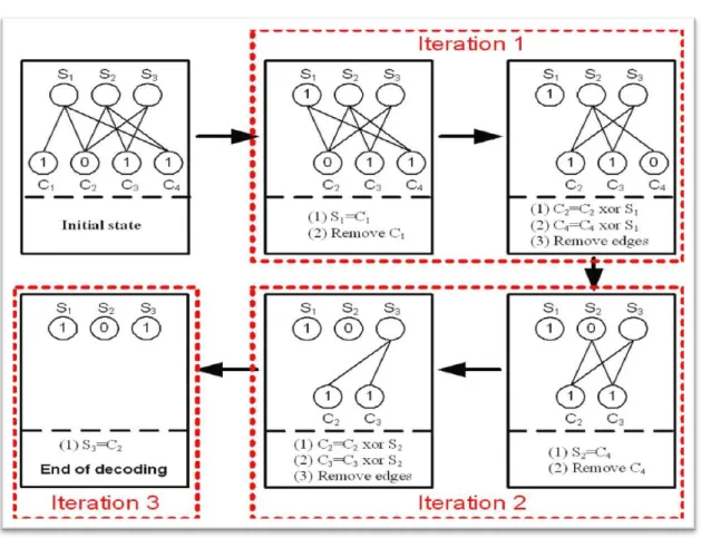
2.1.2. Decoding

The decoding process can be described on a bipartite graph with two sets of nodes presenting source symbols and received encoding symbols [Figure 1]. Initially, one source node and one encoding node have an edge between them if and only if they are neighbors of each other. Values of all source nodes are unknown at the beginning, and values of encoding nodes are set to the corresponding encoding symbols. The decoding process is described as

(11)

3

following:

1. Find a degree-one encoding node 𝑡, i.e. an encoding symbol with only one edge. The process stops when no more degree-one encoding node can be found.

2. Set value of 𝑠, the unique neighbor source symbol of 𝑡, equal to value o f 𝑡. 3. Propagate value of 𝑠 to all neighbors of 𝑠 by adding (exclusive-or) value of 𝑠 to

all neighbors.

4. Remove all edges connected to 𝑠 5. Repeat from step 1.

Figure 1 Decoding process of LT codes

Typically, the goal of the process is to recover all the source nodes. When the process is stopped with some source node still unrecovered, the only way to resume decoding is to receive more encoding symbols to produce additional degree-one node.

(12)

4

2.1.3. Degree Distributions

Degree Distribution determines the performance of LT code. Let ωd be the probability

that the degree of an encoding symbol is 𝑑, i.e. the value of the encoding symbol is exclusive-or of 𝑑 source symbols, 1 ≤ 𝑑 ≤ 𝑘 if there are 𝑘 source symbols. Notice that ∑kd=1ωd 1 , since it is a probability distribution.

Two analytically optimal degree distributions have been proposed in [1] by Luby when he first proposed LT codes. Ideal Soliton Distribution aims to keep expected number of degree-one encoding nodes equal to one at every step in the decoding process, which forms beautiful formulas but works poorly in practice. Robust Soliton Distribution modifies Ideal Soliton Distribution in way to keep the expected number of degree-one nodes equal to 𝑆, instead of 1, to prevent the number of degree-one nodes from reaching zero in the middle of decoding process. However, Robust Soliton Distribution would perform well only when 𝑘 is large (≥ 104).

2.1.4. LT Codes in Raptor Codes

Raptor Codes [2] was proposed as extension of LT Codes. The concept of Raptor Codes is concatenating a high-rate linear block pre-coder with LT Code. Once the fraction of unrecovered source symbols is reaching the capability of pre-coder, the precoder can take over and further decode remaining unrecovered symbols. Therefore, the goal of LT Codes in Raptor Codes is to decode most, but not necessary all, source symbols with small overhead.

2.2. Performance Formulation of LT Codes

2.2.1. Overhead

In traditional scenario of LT codes, the transmitter keeps generating and broadcasting new encoding symbols, while receiver keeps receiving until fully decoded. Since at least 𝑘

(13)

5

encoding symbols are needed to decode all 𝑘 source symbols, the ratio of number of redundant symbols to 𝑘, ε is used as expression of how many redundant symbols are needed, where 𝑘(1 + ε) is the actual number of encoding symbols.

Since LT codes are randomized codes, value of ε is changing case by case. Therefore, averaged ε is the index of performance, which makes perfect sense for scenario like asynchronous broadcasting. For the reason that the transmitter keeps broadcasting new symbols, small chance of large ε is acceptable. However, it is not the case for scenarios like live video streaming/broadcasting. Certain performance requirements for some fixed ε are preferred.

2.2.2. Failure Ratio

Another different requirement is that complete decoding of all source symbols may not be needed. The most obvious example is raptor code mentioned in 2.1.4.

Define failure ratio 𝑟 as the fraction of unrecovered source symbols, i.e. 𝑟 1 − (number of decoded source symbols)/𝑘. Again, 𝑟 is also random, even with fixed 𝜀. Define 𝑅𝜀 as the random variable of failure ratio with fixed 𝜀. Some previously proposed

optimization methods for LT codes used average of failure ratio, i.e. E[𝑅𝜀], as optimization

objective, but produced impractical result, since the value of 𝑅𝜀 can be far away from its

mean.

2.2.3. Failure Probability p

Raptor codes give us the hint of real definition of decoding failure. In Raptor codes, decoding is considered a failure only when the failure ratio exceeds the capacity of pre-coder. Therefore, the failure probability 𝑝 should be the probability that 𝑅𝜀 exceeds certain

(14)

6

2.3. Related works

2.3.1. Finite-Length Analysis of LT Codes

Since robust soliton distributions perform poorly when the code length is short, Karp, Luby and Shokrollahi [3] has provided an efficient method for analyzing error probability of finite-length LT codes. Given degree distribution, error probability can be estimated by recursively calculating probabilities of every possible state during the decoding process of decoder of LT codes . However, the great quantity of states, roughly O(k3), makes it very difficult to find suitable degree distribution analytically.

2.3.2. Importance Sampling Approach

Hyytiä, Tirronen and Virtamo [4] have proposed an algorithm to optimize LT degree distribution

by estimating local gradient empirically. By using the concept of importance sampling the other way

around, they can accurately estimate local gradient of the objective function in the parameter space, and

use the gradient to find better degree distributions iteratively. However, objective functions applicable

to this method are limited to expected value of statistic(s) of individual LT trails. Thus, this method can

only optimize "average" behavior of LT, like average number of encoding symbols needed for

successful decoding, average erasure rate with certain overhead, etc..

2.3.3. Evolution Strategies Approach

Using Evolution Strategies to optimize LT degree distribution was proposed by Chih-Ming Chen, Ying-ping Chen, Tzu-Ching Shen and J.K. Zao [5]. Besides averaged overhead, averaged failure ratio at certain 𝜀 is also used as optimization objective. However, the optimized value of averaged failure ratio does not guarantee the performance, due to bimodal phenomenon of Rε.

(15)

7

Chapter 3. Experiment Setup

3.1. Space of Degree Distribution

With fixed tabs of degrees d1 𝑑2 … 𝑑𝑁, the degree distribution (ωd1 ωd2 … ωdN)

has two constrains: ∑𝑁𝑖=1𝜔𝑑𝑖 1 and ωdi ≥ 0 ∀i ∈ [1 2 … N]. In other words, the space

of degree distribution is an (N-1)-dimensional hyper-plane ωd1+ ωd2 + ⋯ + ωdN 1 in

the all-positive orthant of N-dimensional space. [] handled this problem by normalizing all sample points into the hyper-plane, which introduces a “hollow” dimension to the algorithm, causing increasing of computation complexity and chance to be trapped into local minimum.

Instead of using the hyper-plane, we use the projection of the hyper-plane on the subspace of the first (N-1) dimensions with mapping

f(ω_d₁ ω_d₂ … ω_d_N−1) (ω_d₁ ω_d₂ … ω_d_N−1 1 − ∑𝑁−1𝜔_𝑑_𝑖

𝑖=1 )

. Note that f is a 1-to-1, onto, continuous mapping from the (N-1)-dimensional projection {(ω_d₁ ω_d₂ … ω_d_N−1)|ω_d_i ≥ 0 𝑎𝑛𝑑 ∑𝑁−1𝜔_𝑑_𝑖

𝑖=1 ≤ 1} to the degree distribution space. Thus,

structures like gradient would be preserved when concatenating f with the objective functions.

3.2. Objective Function

Given the definition of failure probability [2.2.3], the most obvious objective function for optimization is to minimize 𝑝 with fixed 𝑟 and 𝜀. However, all three parameters can be used as objective function. With fixed 𝑝 and 𝑟, minimizing required 𝜀 is also reasonable. Among 𝜀 𝑟 and 𝑝, two of the parameters are fixed while the third one being optimized.

(16)

8

3.3. Optimization Parameters

To study behavior of optimizing the three parameters, we choose some typical values of the parameters and run the optimizations with generic optimization algorithms.

Parameter values 0.03 0.06 0.1 0.13 0.16 0 0.001 0.01 0.1 0.0001 0.001 0.01 0.1

Table 1 Typical values of optimization parameters

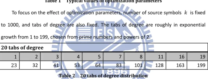
To focus on the effect of optimization parameters, number of source symbols 𝑘 is fixed to 1000, and tabs of degree are also fixed. The tabs of degree are roughly in exponential growth from 1 to 199, chosen from prime numbers and powers of 2.

20 tabs of degree

1 2 3 4 5 7 8 11 16 19

23 32 41 53 64 83 101 128 163 199

Table 2 20 tabs of degree distribution

For each evaluation of objective function, we run the simulations 10000 times to obtain histograms of 𝑅𝜀 and calculate corresponding 𝜀 𝑟 and 𝑝 values.

3.4. Optimization Algorithm

In this thesis, we use two generic optimization algorithms to study the effect of our objective functions. Both algorithms are based on evolution strategies, but treating the parameter space very differently.

3.4.1. Covariance Matrix Adaptation Evolution Strategy

(17)

9

parameter space is a simple Euclidian space, and looks for optimal solution by adapting the covariance matrix during the process of evolution strategy. CMA-ES does not require any information, even existence, of gradient of the fitness function.

3.4.2. Natural Evolution Strategy

Unlike CMA-ES, Natural Evolution Strategy, aka NES, assumes that the parameter space can be non-Euclidian space. Furthermore, NES looks for optimal solution by estimating natural gradients, the gradient on non-Euclidian space, during the process.

(18)

10

Chapter 4. Experiment Results

4.1. - - Space

For each of the optimization experiments, two of the three parameters are fixed, while the other one gets optimized. Therefore, for each optimization experiment, we get an optimal point in the 𝜀-𝑟-𝑝 space. Despite the choice of optimized parameter, all points create one consistent surface in the 3D space.

Figure 2 Optimization results in - - space

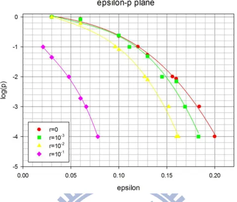
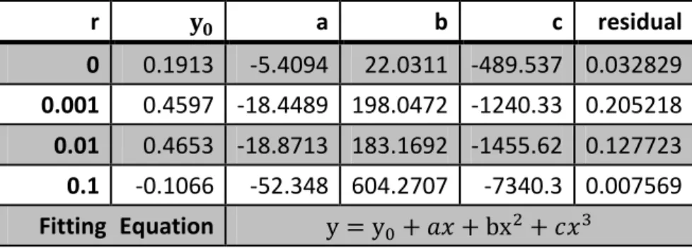
To study the shape of the surface, we cut the surface into sections in two different directions. On the ε-p plane [Figure 3], cubic polynomials fit the optimized points well. On the r-p plane [Figure 4], the shapes of data are similar to inverse third order polynomials (y y0+𝑎_𝑥+_xb2+

𝑐

𝑥3). Curve fitting parameters are shown in Table 3 and Table 4, where the

(19)

11

Figure 3 Optimization results in - - space, projected on - plane

(20)

12 r a b c residual 0 0.1913 -5.4094 22.0311 -489.537 0.032829 0.001 0.4597 -18.4489 198.0472 -1240.33 0.205218 0.01 0.4653 -18.8713 183.1692 -1455.62 0.127723 0.1 -0.1066 -52.348 604.2707 -7340.3 0.007569 Fitting Equation y y₀+ 𝑎𝑥 + bx2+ 𝑐𝑥3

Table 3 Curve fitting parameters of Figure 3

e a b c residual 0.03 1.0943 6.1284 11.3651 7.5881 0.096237 0.06 0.751 4.5739 9.0469 7.9246 0.073963 0.1 2.689 18.804 35.3878 25.9939 0.027227 0.13 3.388 26.7799 50.8833 38.5742 6.66E-05 0.16 -3.2535 -7.9201 -3.9663 29.7197 1.97E-31 Fitting Equation y y0+ 𝑎 𝑥+ b x2+ 𝑐 𝑥3

Table 4 Curve fitting parameters of Figure 4

4.2. Optimized Performance

We use three different graphs to describe the performance of LT codes:  Histograms of 𝑅𝜀

 𝜀 vs. 𝑝 curves  𝜀 vs. 𝑟 curves

By comparing the graphs of different optimized LT codes, we discovered that the behavior of optimized LT codes is determined by the optimized values of r, ε and p, despite the choice of parameter as objective function. Therefore, the behavior of optimized LT codes is determined by position of the code on the 3D surface.

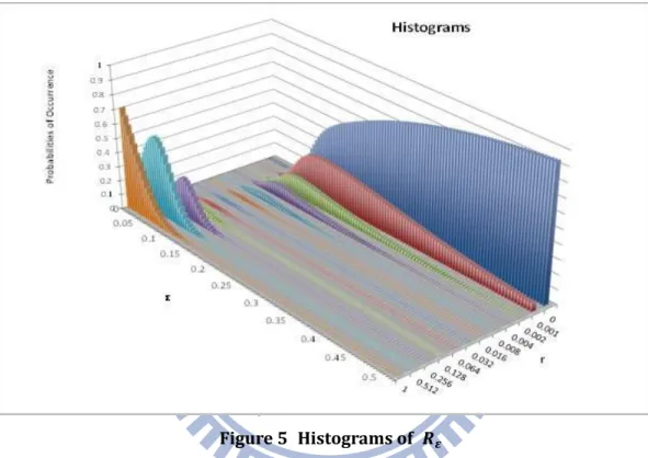
4.2.1. Histograms of

(21)

13

Note that to emphasize the behavior of 𝑅𝜀 at the lower end, the bins grow exponentially

from 0 to 1; that is, the histograms are finer with small 𝑅𝜀 values.

Most of degree distributions exhibit bimodal distribution in histograms of 𝑅𝜀. As Shown

in Figure 5, when ε is close to zero, the histogram concentrates at high r. Instead of moving toward the lower end, the peak at high r declines and another peak at lower r appears and grows as ε increases.

Figure 5 Histograms of

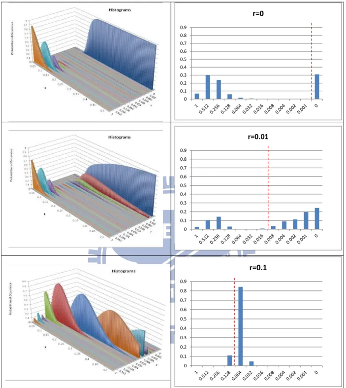
The position of the lower peak is majorly determined by optimized value of r. As the value of r gets more and more strict, the lower peak gets sharper and closer to zero, and two peaks get more separated from each other. On the contrary, if the optimized value of r is getting higher, the two peaks become closer, and even tend to merge with each other.

(22)

14

Figure 6 Histograms with different

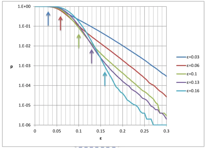
4.2.2. Curves of Failure Probabilities

The 𝜀 vs. 𝑝 curves show the trends of failure probabilities respecting certain 𝑟. By definition, lower curves would have higher r, and curves with different r never intersect. When a degree distribution is said to be optimal with certain 𝑟, 𝜀 and 𝑝, only the curve, corresponding to 𝑟, is optimized at the point (𝜀 𝑝).

0 0.1 0.2 0.3 0.4 0.5 0.6 0.7 0.8 0.9 r=0 0 0.1 0.2 0.3 0.4 0.5 0.6 0.7 0.8 0.9 r=0.01 0 0.1 0.2 0.3 0.4 0.5 0.6 0.7 0.8 0.9 r=0.1

(23)

15

With fixed r, lower optimized 𝜀 (corresponding to higher optimized 𝑝) implies that the curve starts to decrease earlier but its slope is rather moderate. Figure 7 shows that the curve is optimal only at the optimized point, comparing with degree distributions optimized at other points. Therefore, it is a tradeoff between the start point of decreasing and the slope of decreasing.

Figure 7 Failure Probabilities, optimized with different ,

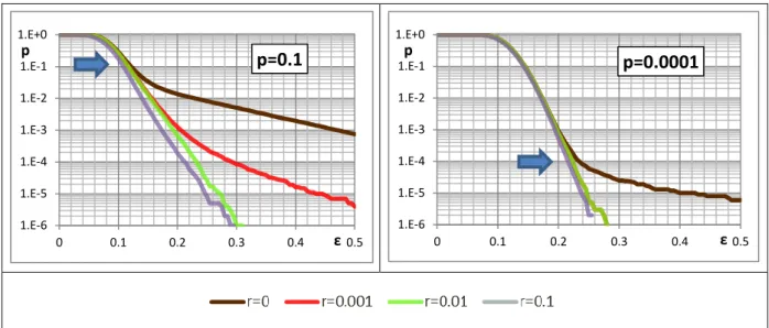
When considering curves (of the same degree distribution) with different r, the lower curves get close to the optimized curve before the optimized point, but tend to disperse afterward [Figure 8]. The upper curves, comparing with the lowers, are always away from the optimized curve [Figure 9]. Since the failure probability is actually cumulative probability of 𝑅𝜀, curves getting close at certain ε somewhat imply that 𝑅𝜀 is bimodal at that ε.

1.E-06 1.E-05 1.E-04 1.E-03 1.E-02 1.E-01 1.E+00 0 0.05 0.1 0.15 0.2 0.25 0.3 p ε ε=0.03 ε=0.06 ε=0.1 ε=0.13 ε=0.16

(24)

16

Figure 8 Failure Probabilities, optimized with different , .

Figure 9 Failure Probabilities, optimized with different , .

1.E-6 1.E-5 1.E-4 1.E-3 1.E-2 1.E-1 1.E+0 0 0.1 0.2 0.3 0.4 0.5 p ε p=0.1 1.E-6 1.E-5 1.E-4 1.E-3 1.E-2 1.E-1 1.E+0 0 0.1 0.2 0.3 0.4 0.5 p ε p=0.0001 1.E-6 1.E-5 1.E-4 1.E-3 1.E-2 1.E-1 1.E+0 0 0.1 0.2 0.3 0.4 0.5 p ε r=0.1 1.E-6 1.E-5 1.E-4 1.E-3 1.E-2 1.E-1 1.E+0 0 0.1 0.2 0.3 0.4 0.5 p ε r=0.01 1.E-6 1.E-5 1.E-4 1.E-3 1.E-2 1.E-1 1.E+0 0 0.1 0.2 0.3 0.4 0.5 p ε r=0.001 1.E-6 1.E-5 1.E-4 1.E-3 1.E-2 1.E-1 1.E+0 0 0.1 0.2 0.3 0.4 0.5 p ε r=0

(25)

17

4.2.3. Curves of Failure Ratios

Given 𝜀 and 𝑝, the corresponding 𝑟 is actually finer percentile of 𝑅𝜀. For example,

when p 0 1, corresponding r is equivalent to 90th percentile. In the 𝜀 vs. 𝑟 graphs, each curve corresponds to different value of p. Note that the r value of curve reaching zero cannot be plotted in logarithmic scale. The curve of averaged r, i.e. E[Rε], is also plotted for

reference [Figure 11].

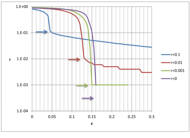
Figure 10 Curves of failure ratios, optimizing with different , .

Like the curves of failure probabilities, only one certain point of one certain curve is optimized when we optimize the three performance parameters. For most of optimized degree distributions, the 𝜀 vs. 𝑟 curves are waterfall-shaped, and the curve corresponding to optimized p has the waterfall ending at the optimized point (ε r) [Figure 10].

Despite the curve corresponding to optimized r, other curves have similar waterfall shape, end at similar r value but different ε value [Figure 11]. The vertical gaps between curves indicate bimodal distribution of Rε. Note that for those degree distributions with

1.E-04 1.E-03 1.E-02 1.E-01 1.E+00 0 0.05 0.1 0.15 0.2 0.25 0.3 r ε r=0.1 r=0.01 r=0.001 r=0

(26)

18

high optimized r, the bimodal phenomena seem gone if look at the histograms. But the curves of failure ratios suggest that the bimodal phenomena are just advanced to lower, even negative ε [Figure 12].

Figure 11 Curves of failure ratios, optimizing with .

Figure 12 Curves of failure ratios, optimizing with .

1.E-5 1.E-4 1.E-3 1.E-2 1.E-1 1.E+0 0 0.05 0.1 0.15 0.2 0.25 0.3 r ε Average r p=0.1 p=0.01 p=0.001 p=0.0001 p=0.9 1.E-2 1.E-1 1.E+0 0 0.05 0.1 0.15 0.2 0.25 0.3 r ε Average r p=0.1 p=0.01 p=0.001 p=0.0001 p=0.9

(27)

19

4.3. Optimized Degree Distributions

4.3.1. Tab of Degree Two

Despite the optimized values of r, ε and p, the tab of degree two has always the highest probability, which is around 0.5±10%. This result is consistent with other researches [1,2]. This indicates that high probability of degree two is essential for efficient LT codes.

4.3.2. Highest Degree

Among all 20 tabs of degree, some tabs have insignificant probabilities. A tab of degree is said to be significant if the probability is higher than 1/199, that is, one over the maximum degree of all 20 tabs. The highest degree, or d𝑚𝑎𝑥, is defined as the highest degree of all the

significant degrees. We found out that highest degree has strong relationship with the optimized value of r.

By observing the highest degrees of degree distributions on the 3D surface [Figure 13], it is obvious that degree distributions with the same r have roughly the same highest degree. The relation between highest degree and r is roughly linear in logarithm scale [Figure 14]. The relation can be expressed as following: 𝑑𝑚𝑎𝑥 1 868𝑟−0 688. This relation

implies that higher 𝑑𝑚𝑎𝑥 is needed if lower r is desired.

Note that the maximum degree is limited to 199 in our experiments, and most of the data concentrate at few points of 𝑟. As the result, current data may not reveal the true relation between highest degree and r.

(28)

20

Figure 13 Highest degrees on the surface (scaled)

(29)

21

4.3.3. Standard Statistics

Means and standard deviations of degree distributions also exhibit strong trends. Means of degree distributions increase as p decreases, and increase even steeper as r decreases [Figure 15]. Standard deviations show roughly the same trend [Figure 16]. Since we know that the major part of the degree distribution is concentrated around the degree two, larger mean and standard deviation imply that degree distribution is more spread towards high degrees. However, while decreasing r or decreasing p , the degree distributions spread out in different ways..

As shown in Figure 17, the normalized standard deviations, which are standard deviations divided by means, increase as r decreases, and are roughly constants if r is fixed. That is to say, standard deviations increase faster than means when decreasing r, but increase in the same speed as means when decreasing p.

(30)

22

Figure 16 Standard deviations of degree distributions

(31)

23

The skewness of degree distribution shows a little different trend. When r is high (roughly 0.01 and higher), the trend of skewness is quite similar to mean and standard deviation, indicating that the degree distribution spreads out in the form of extending the tail of the distribution towards higher degrees. When r is low, however, the skewness decreases as p decreases, which is opposite to mean and standard deviation. The reason could be, again, the limitation of maximum degree. When r is low, the highest degree reaches the maximum available degree (199) in almost every case. Therefore, when decreasing p, the degree distribution can only increase the probability of the tabs of high degrees, instead of extending the tail to even higher degree.

(32)

24

4.4. Modifying Other Parameters

4.4.1. Reducing Tabs of Degree

We choose 7 tabs from the original 20 tabs of degree for further experiments [Table 5]. The first difference between 20 tabs and 7 tabs is that there are several obvious failure cases while optimizing p with 7 tabs. The failure cases have the resultant p equal or very close to one, that is, the maximum value of p. In other words, the optimization failed to improve p in respect to its initial value. The other factor indicating the failure is that obtained degree distribution characteristics do not comply with expected trends. Despite the failure cases, other cases form similar surface in the 3D space. However, the resultant parameters are less consistent [Figure 19(a)(b)]. The variance of optimization results should be further studied.

The resultant performances, however, are quite similar to 20 tabs cases. Trends of degree distribution, mentioned in 0, are also similar. These results indicate that reducing tabs of degree, surprisingly, have no serious impact on performance.

7 tabs from 20 tabs of degree

1 2 3 4 5 7 8 11 16 19

23 32 41 53 64 83 101 128 163 199

(33)

25

(a)

(b)

Figure 19 Optimization results of 20tabs (cyan) and 7 tabs (magenta) from (a) normal and (b) rotated angle of view

(34)

26

4.4.2. Changing Number of source symbols K

By increasing the number of source symbols K from 1000 to 10000, the optimized values of all three parameters, especially ε, are improved [Figure 20]. Since the range of ε shrinks with larger K, reasonable values of ε for given K may become unreasonable when K is changed.

(35)

27

(b)

Figure 20 Optimization results of K=1000 (cyan) and K=10000 (magenta) from (a) normal and (b) rotated angle of view

4.5. Comparison with Related Works

As mentioned in 2.3, the traditional performance measurement is averaged ε needed for fully decoding. In this thesis, although we are not directly optimizing averaged ε, our codes can still outperform codes designed with previous methods, by carefully selecting r and p. Figure 21 shows averaged ε of (1) robust soliton with σ 0 5 c 0 03, (2) best result from [4], (3) result from [5], optimizing overhead, and (4) proposed method with r 0 p 0 1, optimizing ε. Error bars present 10th/90th percentiles. Our proposed method outperforms others in terms of mean and variation.

(36)

28

Figure 21 Averaged with 10th/90th percentiles as error bars

0 0.05 0.1 0.15 0.2 0.25 (1) (2) (3) (4)

(37)

29

Chapter 5. Conclusion

5.1. Achievements

In this thesis, we propose a general formulation of performance of LT codes for optimization. By optimizing any of the three performance parameters, we obtained results forming a concave surface in the ε-r-p space. The performance of optimized LT code is adjustable by tuning the values of performance parameters. We also find strong relations between optimized value of performance parameters and degree distribution, especially the relation between optimized value of r and the highest degree.

5.2. Future Work

5.2.1. Highest Degree

It has been shown that highest degree is strongly related to the optimized value of r. The limitation of maximum degree in our experiment should be relaxed to allow higher values of the highest degree. More values of r should be also studied to confirm the relation between the highest degree and optimized value of r. Another more aggressive experiment could be optimizing the tabs of degree as well as probabilities of degree distributions.

5.2.2. Variation of Optimization results

Despite the fact that LT codes are randomized codes, evolution strategy itself contains the factor of randomness. We have seen that the results obtained from experiments with 7 tabs of degree are less consistent than corresponding results with 20 tabs of degree. Origin of this inconsistency should be further studied.

(38)

30

5.2.3. Applications of Optimized Degree Distributions

In this thesis, all optimized degree distributions are optimal only at particular ε, which implies that the degree distributions are not optimal at other ε. However, by changing the degree distribution during the process of transmission, the receiver can obtain optimal degree distributions at multiple points of ε.

(39)

31

References

[1] M.Luby, "LT Codes", The 43rd Annual IEEE Symposium on Foundations of Computer Science, pp. 271-280, Vancouver, BC, Canada, November 2002.

[2] Amin Shokrollahi, “Raptor Codes”, IEEE Transactions on Information Theory, Volume 52, Issue 6, pp. 2551-2567, June 2006.

[3] Richard Karp, Michael Luby, Amin Shokrollahi, “Finite length analysis of LT codes”, International Symposium on Information Theory, p. 39, Berkeley, Chicago, USA, June 2004.

[4] Esa Hyytiä, Tuomas Tirronen, Jorma Virtamo, “Optimizing the Degree Distribution of LT Codes with an Importance Sampling Approach”, 6th International Workshop on Rare Event Simulation, October 2006. [5] Chih-Ming Chen, Ying-ping Chen, Tzu-Ching Shen and John K. Zao, “On the Optimization of Degree

Distributions in LT Code with Covariance Matrix Adaptation Evolution Strategy”, IEEE Congress on Evolutionary Computation, pp.1-8, Barcelona, Spain, July 2010

(40)

Appendix

This appendix contains results of experiments with 20 tabs of degree and K equal to 1000, using NES algorithm. Meaning of each part of the result is explained as following.

The name of experiment consists of the parameters of experiment. In the following example, “r0.1_p0.01_e” means “optimizing ε with r = 0.1 and p = 0.01 ”. “K1000_20tabs_NES” means “K = 1000, 20 tabs of degree, using NES algorithm”. The fitness value is the value of the optimized parameter, which is ε in this case. Note that when optimizing p or r, the fitness value is the log value of the parameter.

Degree distribution

Name of experiment and final fitness

Optimized value of r, ε and p

Histograms of Rε

Curves of failure probabilities Curves of failure ratios

(41)

r0_p0.0001_e_K1000_20tabs_NES Fitness value = 0.2 Degree Probability 1 4.143E-02 2 4.500E-01 3 1.677E-01 4 6.394E-02 5 2.366E-02 7 5.316E-02 8 5.814E-02 11 2.322E-02 16 4.858E-03 19 8.780E-03 23 3.354E-02 32 1.521E-02 41 1.513E-03 53 8.878E-03 64 1.013E-03 83 0.000E+00 101 7.905E-03 128 0.000E+00 163 0.000E+00 199 3.702E-02 r 0 ε 0.2 p 0.0001 1.E-6 1.E-5 1.E-4 1.E-3 1.E-2 1.E-1 1.E+0 0 0.1 0.2 0.3 0.4 0.5 r ε

ε vs r

1E-4 1E-3 1E-2 1E-1 1E+0 p r 0 0.1 0.2 0.3 ε 59 59

基於演化計算之最佳短碼長LT碼效能與度數分布之研究

國 立 交 通 大 學

網路工程研究所

碩 士 論 文

基於演化計算之最佳短碼長

LT 碼效能與度數分布之研究

A Study of Performance and Degree Distribution of

Optimal Short-Length LT codes

with Aids of Evolution Strategies

研 究 生： 刁培倫

指導教授： 邵家健

教授

基於演化計算之最佳短碼長

LT 碼效能與度數分布之研究

A Study of Performance and Degree Distribution of

Optimal Short-Length LT codes

with Aids of Evolution Strategies

研 究 生：刁培倫

Student: Pei-lun Diao

指導教授：邵家健

Advisor: Dr. John Kar-kin Zao

國 立 交 通 大 學

網 路 工 程 研 究 所

碩 士 論 文

基於演化計算之最佳短碼長

LT 碼效能與度數分布之研究

學生：刁培倫

指導教授： 邵家健 博士

國立交通大學網路工程研究所碩士班

中文論文摘要

A Study of Performance and Degree Distribution of

Optimal Short-Length LT codes

with Aids of Evolution Strategies

Student: Pei-lun Diao

Advisor: Dr. John Kar-kin Zao

Abstract

致謝

刁培倫

Table of Contents

List of Tables

Chapter 1. Introduction

1.1. Objectives

1.2. Research Approach

1.3. Thesis Outline

Chapter 2. Background

2.1. LT Codes

2.2. Performance Formulation of LT Codes

2.3. Related works

Chapter 3. Experiment Setup

3.1. Space of Degree Distribution

3.2. Objective Function

3.3. Optimization Parameters

3.4. Optimization Algorithm

Chapter 4. Experiment Results

4.1. - - Space

4.2. Optimized Performance

4.3. Optimized Degree Distributions

4.4. Modifying Other Parameters

4.5. Comparison with Related Works

Chapter 5. Conclusion

5.1. Achievements

5.2. Future Work

References

Appendix

ε vs r

ε vs p

ε vs r

ε vs p

ε vs r

ε vs p

ε vs r

ε vs p

ε vs r

ε vs p

ε vs r

ε vs p

ε vs r

ε vs p

ε vs r

ε vs p

國立交通大學

碩士論文

研究生：刁培倫

指導教授：邵家健

研究生：刁培倫

國立交通大學

網路工程研究所

碩士論文

指導教授：邵家健博士